| Issue |
A&A
Volume 651, July 2021
|
|
|---|---|---|
| Article Number | A114 | |
| Number of page(s) | 8 | |
| Section | Cosmology (including clusters of galaxies) | |
| DOI | https://doi.org/10.1051/0004-6361/202141081 | |
| Published online | 28 July 2021 | |
Zipf’s law for cosmic structures: How large are the greatest structures in the universe?
1
Centro Ricerche Enrico Fermi, Via Panisperna 89 A, 00184 Rome, Italy
e-mail: This email address is being protected from spambots. You need JavaScript enabled to view it.
2
Sapienza School for Advanced Studies, “Sapienza”, P.le A. Moro, 2, 00185 Rome, Italy
3
Istituto dei Sistemi Complessi (ISC) – CNR, UoS Sapienza, P.le A. Moro, 2, 00185 Rome, Italy
4
Dipartimento di Fisica Università “Sapienza”, P.le A. Moro, 2, 00185 Rome, Italy
Received:
14
April
2021
Accepted:
12
May
2021
Abstract
The statistical characterization of the distribution of visible matter in the universe is a central problem in modern cosmology. In this respect, a crucial question still lacking a definitive answer concerns how large the greatest structures in the universe are. This point is closely related to whether or not such a distribution can be approximated as being homogeneous on large enough scales. Here we assess this problem by considering the size distribution of superclusters of galaxies and by leveraging the properties of Zipf–Mandelbrot law, providing a novel approach which complements the standard analysis based on the correlation functions. We find that galaxy superclusters are well described by a pure Zipf’s law with no deviations and this implies that all the catalogs currently available are not sufficiently large to spot a truncation in the power-law behavior. This finding provides evidence that structures larger than the greatest superclusters already observed are expected to be found when deeper redshift surveys will be completed. As a consequence, the scale beyond which galaxy distribution crossovers toward homogeneity, if any, should increase accordingly.
Key words: cosmology: observations / large-scale structure of Universe / methods: statistical
© ESO 2021
1. Introduction
The distribution of matter in the universe is one of the most fascinating examples of complex structures (Pietronero & Labini 2005; Labini 2011) and it is surely the one concerning the largest objects ever observed. Indeed, such a distribution has been proven to have power-law correlations, corresponding to a fractal structure with a dimension of D ≈ 2 up to several tens of megaparsecs (Pietronero & Labini 2005). Whether or not it presents a crossover toward homogeneity on larger scales is still a matter of considerable debate (Whitbourn & Shanks 2014; Labini et al. 2014; Conde-Saavedra et al. 2015; Alonso et al. 2015; Pandey & Sarkar 2015; Shirokov et al. 2016; Heinesen 2020; Teles et al. 2021). The fractal behavior of visible matter in the universe corresponds to the fact that galaxies are distributed in a hierarchical manner: They form small groups, which, in turn, aggregate into clusters of galaxies and then subsequently clusters are grouped into larger structures, that is to say superclusters and filaments (De Vaucouleurs 1953; Abell et al. 1989), which are the largest known structures in the universe.
Superclusters are linked by these filaments of galaxies and clusters forming the so-called cosmic web (Bond et al. 1996) or superclusters-void network (Einasto et al. 1980), corresponding to a complex distribution of matter characterized by large voids and connected over-densities (Tully et al. 2014; Pomarède et al. 2017, 2020; Colin et al. 2019).
After the surprising discovery of the cosmic web, much attention has been devoted to the quantitative statistical characterization of such large-scale structures, which represent a fundamental aspect of the observable universe and a key issue for any cosmological theory. Indeed, standard cosmological theories are based on the assumption of a uniform distribution of matter and so the identification of the “end of greatness” of galaxy structures represents a key issue in observational astrophysics. In the present paper, we show that there is no statistical evidence that the available data contain the largest existing structures. In addition, large-scale structures carry important information about the primordial universe and pose intriguing theoretical problems concerning their formation (Einasto et al. 2007; Oort 1983). For these reasons many authors have studied the features of the cosmic web, considering the distribution of voids (Hamaus et al. 2014; Pan et al. 2012; Einasto et al. 2011) and that of superclusters (Einasto et al. 1997), and they have tried to reproduce this complex structure with N-body numerical simulations of theoretical models (Springel et al. 2005).
In the present work, we analyze the large-scale structure of the universe considering the size distribution of galaxy super-clusters and leveraging the properties of Zipf–Mandelbrot law (Mandelbrot 1953; Zipf 1949), which may provide interesting hints as to the greatest size of these objects. Previous analyses have considered Zipf’s scaling for voids (Gaite 2005; Tikhonov 2006), which were found to be well described by this statistical law, and the probability distribution of superclusters size (Chow-Martínez et al. 2014), which was found to be a power law. It is worth noting that cosmological N-body simulations do not show such a power-law behavior (Chow-Martínez et al. 2014) and consequently they miss this feature of the large-scale structure of the universe. On the other hand, to the best of our knowledge, the Zipf–Mandelbrot law for galaxy structures has never been considered. As we discuss below, the first problem to be considered is that of defining a reliable list of a supercluster’s size: We approached this by using different definitions and trying to assess the robustness of the results on different observational catalogs. It is worth pointing out that for the present work no analysis on catalogs obtained by N-body simulation was performed. In particular, we tried to quantify the deviations from a pure Zipf’s law, which represent one of the key elements in this statistical characterization of structures. Indeed, it has been recently shown that such deviations allow one to characterize the upper cutoff of the power-law probability distribution of structures size (De Marzo et al. 2021). It is interesting to note that such a cutoff is indirectly related to the scale up to which the distribution of matter in the universe cannot be approximated as being statistically uniform, providing a complementary quantitative tool beyond that based on the correlation functions analysis.
The paper is organized as follows: In Sect. 2, we shortly recall the definition of Zipf’s law and Zipf–Mandelbrot law, pointing out how the level of deviations from Zipf’s law can be used to obtain a characterization of the upper cutoff of the power-law probability distribution. Then in Sect. 3, we present the supercluster catalogs used in the analysis and we compute Zipf–Mandelbrot parameters for all of them. Section 4 is devoted to the discussion of these results, which are also compared with those obtained for cluster catalogs. A measure of statistical fluctuations is introduced ad applied to the various samples. Finally, Sect. 5 is devoted to our final remarks and conclusions.
2. Zipf’s and Zipf–Mandelbrot’s laws
Zipf’s law (Zipf 1949) is a ubiquitous scaling law which can be considered as a sort of footprint of complexity. Indeed, this law has been observed in many complex socio-economic systems, such as cities, firms, and natural language, as well as in a large number of natural systems, such as earthquakes, solar flares, and lunar craters (Zipf 1949; Newman 2005; Cristelli et al. 2012). Many attempts have been devoted to identify a mechanism capable of explaining all of these manifestations of Zipf’s scaling (Pietronero et al. 2001; Bak et al. 1987; Corominas-Murtra et al. 2015; Tria et al. 2014), but a universally accepted generating process is still missing.
Given a system composed of N objects and denoting by S(k), the size of the kth largest one, Zipf’s law reads
 (1)
(1)
where k is the rank and γ is called the Zipf’s exponent. In the case we are going to consider, S(1) is the size of the largest supercluster, S(2) is that of the second largest one, and so on. Zipf’s law is generally visualized by the so-called rank-size plot, obtained plotting the ordered sequence of the sizes as a function of their position in the sequence: If the rank-size plot is a straight line in the log–log scale, then the system is said to follow Zipf’s law.
Zipf’s law is intimately related to power-law probability distributions. We consider a set of objects whose sizes S are power-law distributed, that is
 (2)
(2)
where c is a normalization constant; the intrinsic upper and lower cutoffs of the distribution are called sm and sM, respectively, and Eq. (2) is satisfied for sm ≤ S ≤ sM. We note that such cutoffs are always present in real systems due to intrinsic limits on the size that an object can have: For instance, a supercluster cannot contain less than a galaxy or more than all of the existing galaxies. Generally a power-law behavior is found only in the tail of the distribution, so in correspondence of the largest objects. It can be proven (Cristelli et al. 2012; De Marzo et al. 2021) that if the underlying probability distribution is a power law, then Zipf’s law is valid asymptotically in the rank, that is
 (3)
(3)
and moreover the Zipf’s exponent γ is related to the exponent α of the distribution P(S) by the following expression (Li 2002)
 (4)
(4)
Real systems often show deviations from Zipf’s scaling law (Cristelli et al. 2012; De Marzo et al. 2021), which can be found at low ranks (for the largest objects) or at high ranks (in correspondence with the smallest elements). The latter may derive from the fact that the distribution has a power-law behavior only in the tail or from selection effects. For instance, we could observe only a fraction of small superclusters due to a selection effect in apparent luminosity.
On the other hand, deviations at low ranks can carry important information about the systems considered and they are usually described in terms of Zipf–Mandelbrot’s law (Mandelbrot 1953), which reads as follows:
 (5)
(5)
Here  bar is defined by the relation
  . Zipf’s law is recovered for Q = 0, while strong deviations from the simple power-law behavior of Eq. (3) at low ranks are found for Q ≫ 1. Deviations at low ranks are related to the level of sampling of the distribution and to the presence of cutoffs: Indeed, as is shown by De Marzo et al. (2021), the parameter Q satisfies
 (6)
(6)
where N is the number of objects in the sample considered. The larger the extent of the distribution given by the ratio between the two cutoffs is, the smaller Q is; whereas the larger N is (i.e., the finer is the sampling), the larger Q is. We note that Zipf’s law may arise in the following two very different ways. First, the absence of deviations can be related to the fact that the sample that is available is too small to allow for the detection of the intrinsic upper cutoff of the distribution. This occurs, for instance, by analyzing the size distribution of earthquakes on small time scales (tens of years) (De Marzo et al. 2021). In this case, gradually enlarging the sample leads to a growth of deviations from a pure Zipf’s law. Second, some systems spontaneously evolve out of equilibrium toward Zipf’s law, as it occurs for cities (De Marzo et al. 2021). In this case, even considering the whole sample composed of all the urban settlements of a given country, deviations from Zipf’s law are absent. In both cases, whenever Zipf’s law is found in a sample consisting of only a fraction of the whole system, the observed maximum cannot be used as an estimate for the intrinsic upper cutoff since it is not possible to determine if the low level of sampling is an intrinsic property of the system or an effect produced by the limited system’s size. Indeed, as is shown in De Marzo et al. (2021), the intrinsic upper cutoff of the probability distribution sM can be expressed as a function of the observed maximum S(1) as
 (7)
(7)
For Q → ∞, the intrinsic upper cutoff coincides with the observed maximum (i.e., the largest observed object); whereas for Q → 0, the upper cutoff diverges, meaning that the sample available is not sufficiently large to infer it.
3. Zipf’s law for superclusters of galaxies
Superclusters of galaxies are the largest objects in the observable universe and they can extend for hundreds of megaparsecs containing thousands of galaxies. In order to study the rank-size relation of superclusters, first of all we have to define a suitable measure of their size. Moreover, if we want to prove that Zipf’s law is a robust feature of the distribution of matter in the universe, such a scaling law should be found independently of the size definition adopted. For these reasons, following the hierarchy of cosmic structures, we considered three different definitions of size:
-
the number of galaxies in the supercluster,
-
the number of groups in the supercluster,
-
the number of clusters in the supercluster.
The main problems of these catalogs are their completeness and the possibile artifacts due to observational selection effects and clustering algorithms. Both of which are not simple to take into account. In order to verify that the properties we have detected are intrinsic properties of superclusters, we have analyzed several catalogs, which have been built by using different procedures. In the following subsections, we discuss the analyses we have performed in detail.
3.1. Number of galaxies
The rank-size plots of superclusters, which are ordered according to the number of galaxies they contain, are reported in Fig. 1a. Four different catalogs have been used: Einasto et al. (2006a,b, 2007), and Liivamägi et al. (2012; which contains two distinct catalogs corresponding to different clustering procedures). We also reported the corresponding fits to Zipf–Mandelbrot law, so as to determine the parameter Q and the extent of the deviations from Zipf’s law. For a detailed explanation of the fitting procedure and of the technique used for determining the uncertainty of the fit parameters, readers can refer to the Appendix A. As it is possible to see, superclusters follow Zipf’s law with negligible deviations at low ranks.
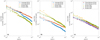 |
Fig. 1. Rank-size plots of superclusters. Panel a: rank-size plots of superclusters ordered by the number of galaxies they contain. Panel b: rank-size plots of superclusters ordered by the number of groups they contain. Panel c: rank-size plots of superclusters ordered by the number of clusters they contain. Solid lines are fits to Zipf–Mandelbrot law, see the Appendix A for details. In all three cases, we observe a pure Zipf’s law with only minor deviations, as is also discussed in the text. |
3.2. Number of groups
Groups are the first level of aggregation of galaxies, for instance the Milky Way is part of the Local Group, which contains approximately 70 galaxies. The catalogs we used for studying the rank-size plot of superclusters, which are ordered by the number of groups they contain, are the same we considered in the previous subsection. The rank-size plots and the corresponding fits to Zipf–Mandelbrot law are reported in Fig. 1b: Also, in this case, only small deviations from Zipf’s law can be detected.
3.3. Number of clusters
Finally, groups of galaxies merge into clusters, which are the level of aggregation just below superclusters. In order to study the adherence to Zipf’s law when superclusters are measured through the number of clusters they contain, we used five catalogs: Einasto et al. (2001), Einasto et al. (2006a,b), Einasto et al. (2007), and Chow-Martínez et al. (2014; which contains two distinct catalogs). The rank-size plots and the corresponding fits to Zipf–Mandelbrot law are reported in Fig. 1c and again the adherence to Zipf’s law is almost perfect.
4. Discussion
In the previous subsection we analyzed the rank-size distribution of superclusters of galaxies considering different definitions of their size and different catalogs. In all cases, negligible deviations from Zipf’s law have been observed. Results are summarized in Table 1, where we also report the minimal value of the deviation parameter Qmin with 95% confidence computed using a parametric bootstrap method (see Appendix A for details). In all cases, the minimum value of Q, that is Qmin, is almost null, meaning that the system we considered is well described by a perfect Zipf’s law, regardless of the definition of size adopted or of the catalog analyzed. As discussed above, this implies that the available data are not sufficient to determine the intrinsic upper cutoff of the distribution of superclusters since, as shown in Eq. (7), this cutoff diverges for Q → 0. In other words, the conclusion is that the observed maximum is a bad estimator of the intrinsic one.
Zipf–Mandelbrot parameters.
This suggests that cosmic structures that are much larger than those contained in the catalogs that we analyzed are likely to be found when larger portions of the universe will be available. Moreover, the absence of a cutoff implies that the distribution of matter in the universe cannot be approximated as homogeneous on the scales of the surveys considered. Indeed, even if a truncation point should exist, the distribution of superclusters is de facto scale invariant up to the largest scales currently observed. We discuss the implications of these results with respect to the standard analysis of homogeneity in the next section.
4.1. Inhomogeneity of the universe
Standard statistical methods based on the determination of the reduced two-point correlation function, or of its Fourier conjugate, are not suitable to test whether a certain distribution is homogeneous in a given sample. The reason is that these statistical tools compare the amplitude of fluctuations to the sample density, that is they assume the sample density to be an unbiased estimator of the density. Such a situation occurs only if the distribution is homogeneous and here the problem arises of testing whether or not a distribution is homogeneous without assuming a priori that this is verified inside a given sample. This point has been discussed at length, for example in Pietronero & Labini (2005), Labini (2011), and we refer the interested reader to those works for a more detailed discussion on the normalization problem.
There is an additional and more subtle problem which may affect any statistical determination in a finite sample, that is even those in which the sample density is an unbiased estimator of the intrinsic average density. Indeed, statistical analyses of finite sample distributions usually assume that fluctuations are self-averaging, meaning that they are statistically similar in different regions of the given sample volume. By determining the conditional density, that is the average galaxy density around a galaxy, Labini et al. (2009a,b) have tested whether this assumption is satisfied in several subsamples of the Sloan Digital Sky Survey (SDSS). The result being that the probability density function (PDF) of conditional fluctuations, filtered on large enough spatial scales (i.e., r > 30 Mpc h−1), shows relevant systematic variations in different subvolumes of the survey. Instead for scales r < 30 Mpc h−1, the PDF is statistically stable, and its first moment presents scaling behavior with a negative exponent around one. Thus, while up to 30 Mpc h−1, galaxy structures have well-defined power-law correlations; on larger scales, it is not possible to consider whole sample average quantities as meaningful and useful statistical descriptors of intrinsic statistical properties. The conclusion of these studies was that this situation is due to the fact that galaxy structures correspond to density fluctuations which are too large in amplitude and too extended in space to be self-averaging on such large scales inside the sample volumes: The galaxy distribution is thus inhomogeneous up to the largest scales, that is r ≈ 100 Mpc h−1, probed by the SDSS samples. It is worth pointing out that the self-averaging property is a necessary, but not sufficient, condition for the distribution of matter to be homogeneous. Indeed, as aforementioned, even if up to 30 Mpc h−1 galaxy structures are self-averaging, they still present power-law correlations and thus a fractal behavior, that is all but homogeneous.
As we are going to show in what follows, the lack of the self-averaging property is related to the absence of deviations from Zipf’s law for superclusters. Indeed, as we have pointed out, Zipf’s law corresponds to an under-sampled probability distribution and, consequently, splitting the sample worsens the level of sampling. This implies that when moving from subsample to subsample, strong fluctuations are expected. In order to show this, we introduced a measure of the large-scale statistical fluctuations of the sample, R. Given a sample divided in M subsamples, this parameter is defined as
 (8)
(8)
where sm(1) is the size of the largest element contained in the mth subsample. For R = 1 all subsamples present similar large-scale structures, while for R > 1 fluctuations appear.
First of all, we consider the case M = 2, which corresponds to splitting the sample in two halves, and we suppose that the system obeys Zipf–Mandelbrot law as seen in Eq. (5). The size of the kth largest structure satisfies
and, as a consequence, it holds
![Mathematical equation: $$ \begin{aligned} {\left\{ \begin{array}{ll} \text{Prob}\left[{R=\left({\frac{2+Q}{1+Q}}\right)^{\gamma }}\right]=\frac{1}{2}\\ \text{Prob}\left[{R=\left({\frac{3+Q}{1+Q}}\right)^{\gamma }}\right]=\left({\frac{1}{2}}\right)^2\\ \vdots \\ \text{Prob}\left[{R=\left({\frac{n+Q}{1+Q}}\right)^{\gamma }}\right]=\left({\frac{1}{2}}\right)^{n-1}.\\ \end{array}\right.} \end{aligned} $$](/articles/aa/full_html/2021/07/aa41081-21/aa41081-21-eq12.gif)
The mean fluctuation parameter ⟨R⟩ is then
This quantity is plotted as a function of Q and for different values of γ in Fig. 2a. As can be seen, the larger Q is, the larger the level of sampling of the inherent distribution is, and the lower the level of fluctuations is. The values of γ measured in the catalogs are in the range γ ∈ [0.4, 0.8]; then for Q = 0, that is, for a perfect Zipf’s law, we have 1.5 < R < 2.5. This implies that one subsample contains, on average, a structure that is between 50% and 150% larger than the largest structure of the other set. We then conclude that in absence of deviations from Zipf’s law, the two subsamples are consistently different when looking at the scale of superclusters.
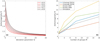 |
Fig. 2. Inhomogeneity. Panel a: average large-scale fluctuations of two subsamples as a function of the deviation parameter Q and for various values of Zipf’s exponent γ. The index R is defined as the ratio between the size of the largest structure in the first subsample and that of the largest structures in the second subsample. In this way, R = 1 corresponds to the absence of large-scale fluctuations. Panel b: fluctuations of the four catalogs we analyzed in Fig. 1a when they are divided in M subgroups. In this case, the ratio was computed between the size of the largest structure and the size of the largest structure of subsample m, where m is the subsample with the smallest largest structure, compared to the other subsamples. The dotted line is the fluctuation parameter of a synthetic sample of 100 sizes, which perfectly adhere to Zipf’s law with exponent γ = 0.6. |
Things worsen if we divide the sample in M > 2 groups, as is shown in Fig. 2b. In this case, we plotted the parameter R determined in the four catalogs we analyzed in Sect. 3.1 for increasing values of M, that is when the sample is divided into more and more subsets. It is possible to see that the larger M is, the larger R is; in particular, for M = 16, the large-scale statistical fluctuation parameter R ranges from 6 (Liivamägi et al. 2012) to 16 (Einasto et al. 2007). We note that this implies that if we split the observed distribution of matter into 16 subsamples, one of them would contain, on average, a structure up to 16 times bigger that the largest supercluster contained in the other subsamples. This indicates that at the scale of superclusters, so at scales of about one hundred megaparsecs, the distribution of matter is not self-averaging and that consequently it cannot be approximated as being statistically uniform. In the same figure, we also plotted (black dotted line) the fluctuation parameter R obtained for a synthetic sample composed of N = 100 structures, which perfectly adhere to Zipf’s law with the exponent γ = 0.6 and in absence of any statistical noise.
4.2. Clusters of galaxies
A natural issue to investigate is the behavior of the distribution of matter in the universe when looked at smaller scales. This can be done, for instance, by analyzing the rank-size distribution of clusters instead of that of superclusters. To this aim, we considered two large datasets: the first is described in Hao et al. (2010) and the second is described in Wen et al. (2012). The corresponding rank-size plots and the corresponding fits to Zipf–Mandelbrot law are reported in Fig. 3a: It is possible to see that there are strong deviations from Zipf’s law. The deviation parameters Q with their minimum value at 95% confidence and Zipf’s exponents γ, are reported in Table 2. In both cases Q is not compatible with a null value, meaning that at the level of aggregation of clusters, the cutoff of the distribution is clearly visible and the distribution itself is completely sampled. Consequently we do not expect to observe clusters much richer than those already observed when larger portions of the universe will be mapped. Moreover, as discussed above, the presence of strong deviations from Zipf’s law also implies that at the scales of clusters, that is on scales of a few megaparsecs, the distribution of matter is self-averaging, confirming previous findings (Labini et al. 2009a,b). Indeed, as is shown in Fig. 3b, the inhomogeneity parameter R, as seen in Eq. (8), is much smaller than that obtained in the case of superclusters, as can be seen in Fig. 2b, since its value is less than 2 when the sample is divided into M = 16 groups. We also plotted (black dotted line) the fluctuation parameter of a synthetic sample composed on N = 1000 elements described by a Zipf–Mandelbrot law with parameters γ = 0.27, Q = 5, and in the absence of any statistical noise. Again, we note that this does not imply that on small scales the distribution of matter is homogeneous, but only that it is self-averaging. Indeed, previous studies have shown that galaxy structures are fractal on the scale of galaxy clusters.
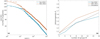 |
Fig. 3. Clusters of galaxies. Panel a: rank-size plots of galaxy clusters measured by the number of galaxies they contain. In this case, there are strong deviations from Zipf’s law for both the catalogs we considered. Panel b: large-scale statistical fluctuations in parameter R of the two catalogs as a function of the number of groups M. Even when M is large, the parameter R is close to one. This implies that no strong fluctuations are observed. The black dotted line is the fluctuation parameter of a synthetic set of N = 103 elements, which adhere to Zipf–Mandelbrot law with parameters γ = 0.27, Q = 5, and no statistical noise. |
Clusters of galaxies.
5. Conclusions
The determination of the properties of the distribution of matter in the universe is one of the most important and challenging problems in modern cosmology since the presence of large-scale structures of galaxies may be in contrast with the “end of greatness”. This distribution shows a power-law correlation, corresponding to a fractal behavior with the dimension D ≈ 2 up to tens of megaparsecs; it is thus natural to asses statistical properties of such a distribution using the tools of complex systems. Many works have gone in this direction after the finding that matter in the universe is characterized by a complex hierarchical structure rather than being spread in a statistically uniform way; here we present a novel approach to the problem based on Zipf’s law. In particular we focus on galaxy superclusters, the largest structures in the universe, assessing their adherence to Zipf–Mandelbrot law.
Considering several catalogs and different definitions of the supercluster size, we found out that superclusters show Zipf–Mandelbrot law with the deviation parameter Q close to zero, meaning that they almost perfectly adhere to Zipf’s law. This finding has several implications as follows.
-
Despite the catalogs we considered are the largest currently available, they do not show the presence of an intrinsic upper cutoff of the probability distribution of superclusters, that is they consequently scale free up to the sizes of the largest structures observed.
-
The absence of an intrinsic cutoff in the available samples implies that structures much larger than those currently observed are expected to be found as soon as deeper catalogs will be released.
-
The probability distribution of superclusters is only poorly sampled and, as a consequence, different subsamples of the catalogs we considered show different large-scale properties. This implies that the distribution of matter is not self-averaging on the scales of tens of megaparsecs, confirming previous findings, and thus that it cannot be approximated as being homogeneous on such scales.
Exploiting the same methodology, we also analyzed the distribution of matter on smaller scales, considering the distribution of clusters rather that that of superclusters. In this case, strong deviations from Zipf’s law are observed and therefore, on scales of a few megaparsecs, the distribution of matter is self-averaging, confirming previous findings which have also shown this distribution to be fractal on such scales. Our study shows that the self-averaging property is deeply entangled with the level of sampling of the probability distribution of cosmic structures and with the presence of deviations from Zipf’s law. This approach thus provides a novel and complementary vision with respect to those based on the study of the correlation functions or other statistical properties. Moreover it also demonstrates that Zipf’s law, which is often considered as a mere empirical law, can be used to gather fundamental information about systems characterized by a complex structure. The application of this Zipf’s law based analysis to the forthcoming galaxy surveys and to N-body simulated catalogs represent a natural and interesting extension of the study presented in this work. In particular, by following the dynamical evolution of the structures during a numerical simulation, it would be possible to determine if Zipf’s law is an intrinsic feature of superclusters of galaxies or a spurious manifestation of this scaling law (De Marzo et al. 2021).
Acknowledgments
We thanks the referee Professor Bernard Jones for his helpful comments about the manuscript and for his suggestions about possible further studies.
References
- Abell, G. O., Corwin, H. G., Jr, & Olowin, R. P. 1989, ApJS, 70, 1 [NASA ADS] [CrossRef] [EDP Sciences] [Google Scholar]
- Alonso, D., Salvador, A. I., Sánchez, F. J., et al. 2015, MNRAS, 449, 670 [NASA ADS] [CrossRef] [Google Scholar]
- Bak, P., Tang, C., & Wiesenfeld, K. 1987, Phys. Rev. Lett., 59, 381 [NASA ADS] [CrossRef] [PubMed] [Google Scholar]
- Bond, J. R., Kofman, L., & Pogosyan, D. 1996, Nature, 380, 603 [NASA ADS] [CrossRef] [Google Scholar]
- Burroughs, S. M., & Tebbens, S. F. 2001, Pure Appl. Geophys., 158, 741 [CrossRef] [Google Scholar]
- Chow-Martínez, M., Andernach, H., Caretta, C., & Trejo-Alonso, J. 2014, MNRAS, 445, 4073 [NASA ADS] [CrossRef] [Google Scholar]
- Colin, J., Mohayaee, R., Rameez, M., & Sarkar, S. 2019, A&A, 631, L13 [NASA ADS] [CrossRef] [EDP Sciences] [Google Scholar]
- Conde-Saavedra, G., Iribarrem, A., & Ribeiro, M. B. 2015, Phys. A: Stat. Mech. App., 417, 332 [CrossRef] [Google Scholar]
- Corominas-Murtra, B., Hanel, R., & Thurner, S. 2015, Proc. Nat. Acad. Sci., 112, 5348 [CrossRef] [Google Scholar]
- Cristelli, M., Batty, M., & Pietronero, L. 2012, Sci. Rep., 2, 812 [CrossRef] [Google Scholar]
- De Marzo, G., Gabrielli, A., Zaccaria, A., & Pietronero, L. 2021, Phys. Rev. Res., 3, 013084 [CrossRef] [Google Scholar]
- De Vaucouleurs, G. 1953, AJ, 58, 30 [NASA ADS] [CrossRef] [Google Scholar]
- Einasto, J., Jôeveer, M., & Saar, E. 1980, MNRAS, 193, 353 [NASA ADS] [CrossRef] [Google Scholar]
- Einasto, M., Tago, E., Jaaniste, J., Einasto, J., & Andernach, H. 1997, ApJS, 123, 119 [Google Scholar]
- Einasto, M., Einasto, J., Tago, E., Müller, V., & Andernach, H. 2001, AJ, 122, 2222 [CrossRef] [Google Scholar]
- Einasto, J., Einasto, M., Saar, E., et al. 2006a, VizieR Online Data Catalog: J/A+A/459/L1 [Google Scholar]
- Einasto, J., Einasto, M., Saar, E., et al. 2006b, A&A, 459, L1 [NASA ADS] [CrossRef] [EDP Sciences] [Google Scholar]
- Einasto, J., Einasto, M., Tago, E., et al. 2007, A&A, 462, 811 [NASA ADS] [CrossRef] [EDP Sciences] [Google Scholar]
- Einasto, J., Suhhonenko, I., Hütsi, G., et al. 2011, A&A, 534, A128 [NASA ADS] [CrossRef] [EDP Sciences] [Google Scholar]
- Gaite, J. 2005, Eur. Phys. J. B Condens. Matter Complex Syst., 47, 93 [CrossRef] [Google Scholar]
- Hamaus, N., Sutter, P., & Wandelt, B. D. 2014, Phys. Rev. Lett., 112 [Google Scholar]
- Hao, J., McKay, T. A., Koester, B. P., et al. 2010, ApJS, 191, 254 [NASA ADS] [CrossRef] [Google Scholar]
- Heinesen, A. 2020, JCAP, 2020, 052 [CrossRef] [Google Scholar]
- Labini, F. S. 2011, CQG, 28, 164003 [NASA ADS] [CrossRef] [Google Scholar]
- Labini, F. S., Vasilyev, N. L., & Baryshev, Y. V. 2009a, A&A, 508, 17 [NASA ADS] [CrossRef] [EDP Sciences] [Google Scholar]
- Labini, F. S., Vasilyev, N. L., Pietronero, L., & Baryshev, Y. V. 2009b, EPL, 86, 49001 [NASA ADS] [CrossRef] [EDP Sciences] [Google Scholar]
- Labini, F. S., Tekhanovich, D., & Baryshev, Y. V. 2014, JCAP, 2014, 035 [CrossRef] [Google Scholar]
- Li, W. 2002, Glottometrics, 5, 14 [Google Scholar]
- Liivamägi, L. J., Tempel, E., & Saar, E. 2012, A&A, 539, A80 [NASA ADS] [CrossRef] [EDP Sciences] [Google Scholar]
- Mandelbrot, B. 1953, Commun. Theory, 84, 486 [Google Scholar]
- Newman, M. E. 2005, Contemp. Phys., 46, 323 [NASA ADS] [CrossRef] [Google Scholar]
- Oort, J. H. 1983, ARA&A, 21, 373 [NASA ADS] [CrossRef] [Google Scholar]
- Pan, D. C., Vogeley, M. S., Hoyle, F., Choi, Y.-Y., & Park, C. 2012, MNRAS, 421, 926 [NASA ADS] [CrossRef] [Google Scholar]
- Pandey, B., & Sarkar, S. 2015, MNRAS, 454, 2647 [NASA ADS] [CrossRef] [Google Scholar]
- Pietronero, L., & Labini, F. S. 2005, Complexity, Metastability and Nonextensivity (World Scientific), 91 [CrossRef] [Google Scholar]
- Pietronero, L., Tosatti, E., Tosatti, V., & Vespignani, A. 2001, Phys. A: Stat. Mech. App., 293, 297 [Google Scholar]
- Pomarède, D., Hoffman, Y., Courtois, H. M., & Tully, R. B. 2017, ApJ, 845, 55 [Google Scholar]
- Pomarède, D., Tully, R. B., Graziani, R., et al. 2020, ApJ, 897, 133 [Google Scholar]
- Shirokov, S., Lovyagin, N. Y., Baryshev, Y. V., & Gorokhov, V. 2016, Astron. Rep., 60, 563 [Google Scholar]
- Springel, V., White, S. D., Jenkins, A., et al. 2005, Nature, 435, 629 [Google Scholar]
- Teles, S., Lopes, A. R., & Ribeiro, M. B. 2021, Phys. Lett. B, 813 [Google Scholar]
- Tikhonov, A. V. 2006, Astron. Lett., 32, 727 [Google Scholar]
- Tria, F., Loreto, V., Servedio, V. D. P., & Strogatz, S. H. 2014, Sci. Rep., 4, 5890 [Google Scholar]
- Tully, R. B., Courtois, H., Hoffman, Y., & Pomarède, D. 2014, Nature, 513, 71 [NASA ADS] [CrossRef] [Google Scholar]
- Wen, Z., Han, J., & Liu, F. 2012, ApJS, 199, 34 [Google Scholar]
- Whitbourn, J., & Shanks, T. 2014, MNRAS, 437, 2146 [Google Scholar]
- White, E. P., Enquist, B. J., & Green, J. L. 2008, Ecology, 89, 905 [Google Scholar]
- Zipf, G. K. 1949, Human behavior and the principle of least effort (Cambridge, MA, Addison-Wesley) [Google Scholar]
Appendix A
Derivation of the expressions for Q and sM
As in De Marzo et al. (2021), we consider a truncated power-law distribution of sizes, P(S), that is
 (A.1)
(A.1)
where c is the normalization constant, and sm and sM are the lower and upper cutoff of the distribution. We recall that in the present case, S coincides with the size of superclusters. These cutoffs are connected to c by the normalization condition
 (A.2)
(A.2)
Now, in considering the PDF P(S) of a continuous variable S, the values of its cumulative distribution function (CDF) C(S) are equiprobable. This is because the CDF is defined as  and so, in performing the change of variable from S → C = C(S) and denoting f(C) as the PDF of C, we get
  for 0 ≤ C ≤ 1. As a consequence, given N values of S are independently extracted from P(S), with good approximation they can be considered as uniformly spaced in the corresponding variable C. Thus, the kth size ranked value S(k) approximately corresponds to the CDF value
  . In formulas
which, together with Eq. (A.2), gives
Making the assumption that N + 1 ≈ N, sM ≫ sm, and in introducing  , we end up with the final rank-size formula
![Mathematical equation: $$ \begin{aligned} S(k)=\left[{\frac{Ns_m^{\frac{1}{\gamma }}s_M^{\frac{1}{\gamma }}}{Ns_m^{\frac{1}{\gamma }} +ks_M^{\frac{1}{\gamma }}}}\right]^{\gamma }= \frac{N^{\gamma }s_m}{\left[{k+N\left({\frac{s_m}{s_M}} \right)^{\frac{1}{\gamma }}}\right]^{\gamma }}\cdot \end{aligned} $$](/articles/aa/full_html/2021/07/aa41081-21/aa41081-21-eq22.gif) (A.3)
(A.3)
By comparing this expression with the Zipf–Mandelbrot law, as seen in Eq. (5),
 (A.4)
(A.4)
it follows that
 (A.5)
(A.5)
These expressions relate the number of values or objects in the system and the parameters of the PDF P(S) on one side, and the Zipf–Mandelbrot parameters on the other. We note that Q not only quantifies deviations from Zipf’s law, but it also quantifies the level of sampling of the inherent distribution. Indeed Q is the larger the wider the statistical sample is, thus the larger the number N of objects in the sample is and it is the smaller the wider the extension of the truncated power law is, given by the ratio between the upper cutoff and the lower one.
Finally, combining Eqs. (A.4) and (A.5), we obtain an expression for the upper cutoff sM
which yields
Fitting procedure and uncertainty assessment
We adopted a standard nonlinear least squares (NLS) fitting procedure to determine the parameters of Zipf–Mandelbrot law. This technique, if applied to the rank-size plot, or, equivalently, to the complementary cumulative distribution, has an accuracy which is comparable to maximum likelihood estimates (White et al. 2008), while being much simpler (Burroughs & Tebbens 2001) if the upper cutoff is unknown. In particular, we used Eq. (5) partially linearized through logarithms

where Q, γ, and c are free parameters. The fitting algorithm returns 95% confidence bounds on these parameters; however, such uncertainty does not take into account statistical fluctuations that are encountered considering different samples generated by the same power-law distribution. For this reason we exploited a parametric bootstrap so as to obtain a more realistic measure of uncertainty. In particular we adopted the following procedure
-
we computed the parameter Q of the empirical data with the NLS technique;
-
we used Eqs. (4) and (6) to determine the parameters of the underlying power-law distribution;
-
we generated M = 1000 Monte Carlo samples with numerosity N as the empirical sample using the power-law distribution obtained in the previous step;
-
each synthetic sample m was fitted with the NLS technique, so as to obtain the parameters Qm;
-
the empirical distribution of Q, P(Q), was obtained by performing a histogram of the M values Qm;
-
starting from the probability distribution P(Q), the confidence bound for Q was easily obtained using the cumulative distribution and determining the interval containing 95% of the probability.
All Tables
All Figures
|
Fig. 1. Rank-size plots of superclusters. Panel a: rank-size plots of superclusters ordered by the number of galaxies they contain. Panel b: rank-size plots of superclusters ordered by the number of groups they contain. Panel c: rank-size plots of superclusters ordered by the number of clusters they contain. Solid lines are fits to Zipf–Mandelbrot law, see the Appendix A for details. In all three cases, we observe a pure Zipf’s law with only minor deviations, as is also discussed in the text. |
| In the text | |
|
Fig. 2. Inhomogeneity. Panel a: average large-scale fluctuations of two subsamples as a function of the deviation parameter Q and for various values of Zipf’s exponent γ. The index R is defined as the ratio between the size of the largest structure in the first subsample and that of the largest structures in the second subsample. In this way, R = 1 corresponds to the absence of large-scale fluctuations. Panel b: fluctuations of the four catalogs we analyzed in Fig. 1a when they are divided in M subgroups. In this case, the ratio was computed between the size of the largest structure and the size of the largest structure of subsample m, where m is the subsample with the smallest largest structure, compared to the other subsamples. The dotted line is the fluctuation parameter of a synthetic sample of 100 sizes, which perfectly adhere to Zipf’s law with exponent γ = 0.6. |
| In the text | |
|
Fig. 3. Clusters of galaxies. Panel a: rank-size plots of galaxy clusters measured by the number of galaxies they contain. In this case, there are strong deviations from Zipf’s law for both the catalogs we considered. Panel b: large-scale statistical fluctuations in parameter R of the two catalogs as a function of the number of groups M. Even when M is large, the parameter R is close to one. This implies that no strong fluctuations are observed. The black dotted line is the fluctuation parameter of a synthetic set of N = 103 elements, which adhere to Zipf–Mandelbrot law with parameters γ = 0.27, Q = 5, and no statistical noise. |
| In the text | |
Current usage metrics show cumulative count of Article Views (full-text article views including HTML views, PDF and ePub downloads, according to the available data) and Abstracts Views on Vision4Press platform.
Data correspond to usage on the plateform after 2015. The current usage metrics is available 48-96 hours after online publication and is updated daily on week days.
Initial download of the metrics may take a while.