| Issue |
A&A
Volume 651, July 2021
|
|
|---|---|---|
| Article Number | A4 | |
| Number of page(s) | 17 | |
| Section | Interstellar and circumstellar matter | |
| DOI | https://doi.org/10.1051/0004-6361/202141002 | |
| Published online | 01 July 2021 | |
Structure and dynamics of the inner nebula around the symbiotic stellar system R Aquarii
1
Observatorio Astronómico Nacional (OAN-IGN),
Apartado 112,
28803
Alcalá de Henares,
Spain
e-mail: This email address is being protected from spambots. You need JavaScript enabled to view it.
2
Instituto de Física Fundamental, CSIC,
C/ Serrano 123,
28006
Madrid, Spain
3
Observatorio Astronómico Nacional (OAN-IGN),
C/ Alfonso XII, 3,
28014 Madrid, Spain
4
Korea Astronomy and Space Science Institute,
776,
Daedeokdae-ro, Yuseong-gu,
Daejeon 34055, Republic of Korea
5
Institut de Radioastronomie Millimétrique,
300 rue de la Piscine,
38406
Saint Martin d’Hères, France
6
Nicolaus Copernicus Astronomical Center, Polish Academy of Sciences,
ul. Bartycka 18,
00-716
Warsaw, Poland
Received:
6
April
2021
Accepted:
29
April
2021
Abstract
Aims. We investigate the structure, dynamics, and chemistry of the molecule-rich nebula around the stellar symbiotic system R Aqr, which is significantly affected by the presence of a white dwarf (WD) companion. We study the effects of the strong dynamical interaction between the AGB wind and the WD and of photodissociation by the WD UV radiation on the circumstellar shells.
Methods. We obtained high-quality ALMA maps of the 12CO J = 2−1, J = 3−2, and J = 6−5 lines and of 13CO J = 3−2. The maps were analyzed by means of a heuristic 3D model that is able to reproduce the observations. In order to interpret this description of the molecule-rich nebula, we performed sophisticated calculations of hydrodynamical interaction and photoinduced chemistry.
Results. We find that the CO-emitting gas is distributed within a relatively small region ≲1.″5. Its structure consists of a central dense component plus strongly disrupted outer regions, which seem to be parts of spiral arms that are highly focused on the orbital plane. The structure and dynamics of these spiral arms are compatible with our hydrodynamical calculations. We argue that the observed nebula is the result of the dynamical interaction between the wind and the gravitational attraction of the WD. We also find that UV emission from the hot companion efficiently photodissociates molecules except in the densest and best-shielded regions, that is, in the close surroundings of the AGB star and some shreds of the spiral arms from which the detected lines come. We can offer a faithful description of the distribution of nebular gas in this prototypical source, which will be a useful template for studying material around other tight binary systems.
Key words: stars: AGB and post-AGB / circumstellar matter / binaries: close / binaries: symbiotic / stars: individual: R Aqr
© ESO 2021
1 Introduction
Symbiotic stellar systems (SSs) are tight binary systems that typically consist of an evolved asymptotic giant branch star (the AGB primary, very bright) and a white dwarf (WD, the secondary), in which strong interactions are taking place, see, for instance, Mikołajewska (2012). The AGB wind is found to be strongly disrupted by the interaction, and an active accretion disk is formed around the secondary WD, leading to the ejection of very fast jets and nova-like phenomena. The study of SSs is essential for understanding all interacting binaries that include evolved giants, in which the symbiotic-like activity is usually much more elusive to observers, with implications for the formation of bipolar planetary nebulae, the interaction of nova ejecta with circumstellar material, the formation of chemically peculiar stars, and the progenitors of type Ia supernovae.
The gravitational interaction between the wind from the primary and the compact secondary is thought to be the dominant phenomenon that explains the SS activity, and it is expected to deeply shape the circumstellar wind nebula (e.g., Mohamed & Podsiadlowski 2012; de Val-Borro et al. 2017; Saladino et al. 2018; Kim et al. 2019). Hydrodynamical calculations show the efficiency of a mass-transfer mode called wind Roche-lobe overflow (WRLOF), which occurs when the wind velocity is still moderate when it reaches the surroundings of the secondary, which significantly reinforces the companion-wind interaction. After the interaction, the AGB-star wind is predicted to be strongly focused on the binary orbital plane and to form spiral-like arms or arcs.
R Aqr is the best-studied SS. The primary is a bright Mira-type variable, and the companion is a WD. The nebula with size of 2′ consists of an equatorial structure that is elongated in the east-west direction and a precessing jet (with a position angle, PA, ranging between 10° and 45°) powered by the accretion onto the WD; see Solf & Ulrich (1985), Melnikov et al. (2018), and references therein. The orbital parameters have recently been reanalyzed using new measurements of the relative stellar positions and significantly more accurate measurements of the AGB velocity (Bujarrabal et al. 2018; Alcolea et al., in prep.; Gromadzki & Mikołajewska 2009). The orbit shows a relatively long period, ~ 42 yr, and high eccentricity, with a typical stellar separation equivalent to about 40 mas. At the time of our ALMA observations (2017–2018), the WD was approaching a tight pericenter, which took place by the end of 2019, and it was moving toward the observer at a velocity of about 10 km s−1. For our purposes, it is also important to point out that the orbital plane is roughly perpendicular to the plane of the sky, with its northern hemisphere pointing to us, and that the orbital axis (projected on the plane of the sky) is placed at PA ~ 0–10 degrees. See Alcolea et al. (in prep.) and Sect. 4.1 for more details.
The properties of the primary are relatively well known. It is a very bright M6.5–8.5 Mira-type variable, with a period of about 385 days. A relatively thick circumstellar envelope around it yields a moderate extinction that varies with time in a not straightforward way that is related to the geometry of the system, in particular, to the orbital phase and the stream of gas that is ejected by the Mira primarily onto the orbital plane (Gromadzki & Mikołajewska 2009). Thus, measurements of Av range from 3.1 mag in 1977 (last periastron passage) to 0.5 mag only 5 yr later (Brugel et al. 1984). Intermediate values such as 1.9–2.0 magwere measured in between (Wallerstein & Greenstein 1980; Kaler 1981), and an average of 0.7 mag (excluding high-obscuration events) was found in a period ranging from the mid-1970s to the mid-2000s (Gromadzki et al. 2009). Typical extinction values of about 1–2 mag are therefore expected, but with significant variations with time. The values of the extinction are particularly relevant for estimating the effects of photodissociation (Sect. 4.3), but we recall that the values toward the AGB and the WD can be different and that the extinction also depends on the angle between the equator and the chosen direction (the values given above only refer to the direction toward the Earth, which is not in the equatorial plane).
The compact companion, whose effects on the nebula are expected to be very strong, is more difficult to study because it is barely observable. We discuss its properties in Sect. 4.3, in particular, those that are relevant for our study of CO photodissociation.
Parallax measurements from SiO VLBI data indicate a distance of 218 pc (Min et al. 2014), although the distance from the GAIA parallax is 320 pc; the origin of this discrepancy is unknown. Both measurements are subject to uncertainties because the stellar diameter and the SiO-emitting region are much larger than the measured parallax; in addition, both methods ignore the orbital movements of the mira component. From our analysis of the orbital and stellar parameters, and also accounting for the period-luminosity relations (Alcolea et al., in prep.), we conclude that the most probable value is intermediate between them, ~ 265 pc.
Molecular emission is very rarely observed in SSs, probably due to photodissociation by the UV emission of the WD and its surroundings and strong disruption of the shells, except from regions very close to the AGB. R Aqr is indeed the most intense SS in molecular lines, and its emissions have been relatively well studied (Bujarrabal et al. 2010, 2018). Although the CO lines in R Aqr are much weaker than in standard AGB stars, they have been clearly detected and mapped with ALMA.
In our first ALMA observing run (Bujarrabal et al. 2018; Gómez-Garrido et al., in prep.), we mapped the surroundings of the star in continuum and line emission. We reached suborbital scales in some cases. It is interesting to note that these observations were obtained only three years after the measurement of the stellar positions by Schmid et al. (2017). In this paper, we reanalyze some of our previous results and present new observations of other lines of 12CO, the only molecule showing well-resolved emission with the ALMA angular resolutions (around 30 mas). These data are analyzed by means ofsimple, heuristic modeling, whose main goal is to describe the structure and kinematics that the inner nebula around R Aqr must show to explain the observations. The various nebular components were built by accounting for the results of very detailed hydrodynamical calculations that were specifically performed for our case, and a deep discussion of the chemistry, in particular, of the strong photodissociation effects in this very complex environment.
2 New observations and reanalysis of previous data
We present ALMA maps showing the extended emission of the molecular lines 12CO J = 2−1, J = 3−2, and J = 6−5, as well as maps of the J = 3−2 line of 13CO. Resolutions between 20 and 200 milliarcsec (mas) were attained. Maps of other lines and the continuum will be presented in Gómez-Garrido et al. (in prep.).
The high-resolution 12CO J = 3−2 observations were obtained with ALMA in November 2017 and have been presented by Bujarrabal et al. (2018). We performed a new cleaning of the uv data using a new velocity channel distribution to obtain comparable velocity brightness distributions for all the lines presented here; a small spurious shift in the LSR velocity (with negligible effect on the results) that was present in our previous maps has been corrected. For more details on the data acquisition and calibration, see Bujarrabal et al. (2018). The maps are presented in Fig. 1. The telescope half-power beam width (HPBW) was 40 × 30 mas, and the major axis at PA = 63°. The presented maps are centered on the continuum centroid, which for this line is at ICRS coordinates RA: 23:43:49.4962, Dec: –15:17:04.720.
In the maps of this line, the continuum was subtracted from the line maps (at the stage of uv data), to better show the emission in the weak wings of the line. We proceeded the same way for the rest of the maps presented in this paper, except for the J = 6−5 map (see below). In all our maps, except for the low-resolution J = 3−2 maps, which are mostly interesting to detect weak features, the data were resampled to the same velocity resolution, 0.8 km s−1. Because the movements of the star are complex, with significant and uncertain proper movements and a non-negligible orbit size, we decided to center all our maps on the respective continuum centroids, which were measured independently for each frequency and epoch. We recall that the dependence of the centroid positions on the frequency and epoch of the observations is almost unpredictable. All these effects are discussed in Gómez-Garrido et al. (in prep.). The centroid coordinates will be given in each case, so that the meaning of the shifts can be assessed.
We also present maps of 12CO J = 3−2 obtained in September 2018 with a more compact ALMA configuration, which therefore yield a poorer angular resolution, but with a higher sensitivity (Fig. 2). The calibration of the visibilities was performed using standard procedures with the CASA software. The GILDAS software was used for the subsequent cleaning, for which we used the Hogbom method and the Briggs weighting scheme with a robust value of 1. The HPBW in these observations is 0.″ 17 × 0.″ 14 (PA = 83°). These observations are mainly useful to check the presence of more extended and weaker emission. These high-sensitivity maps confirm the presence of weak southern spots at a distance of between 0.″ 5 and 1″, which were clearly detected and have been already depicted in maps by Ramstedt et al. (2018, with a resolution of 0.″ 38 × 0.″ 33). The southern spots are about 30 times weaker than the brightness peak, and therefore their detection in the high-resolution maps is in principle not expected. These maps are also centered on the corresponding continuum centroid, RA: 23:43:49.4994, Dec: –15:17:04.765.
The comparison of the integrated flux-density profiles, F(Jy), obtained from these low-resolution observations and the wide-configuration observations presented before, indicates a moderate loss of flux in the high-resolution maps of ~ 25% at the central velocities (and ≲35% at 10 km s−1 LSR). There is no published single-dish profile to be compared with our integrated flux, but this moderate flux loss is confirmed by our J = 2−1 maps, see below, whose integrated profile can be compared with single-dish data and shows very similar fluxes. The brightness distributions of all these (J = 3−2 and J = 2−1) maps are completely similar (taking the different resolutions into account and not considering the weak detached spots). We conclude that the flux lost in our high-resolution J = 3−2 maps is moderate,less than about one-third, and that it probably consists of a contour at a level lower than 10% of the peak values (in all the panels of Fig. 1).
Maps of 13CO J = 3−2 observations were simultaneously obtained with the high-resolution 12CO map and were reduced in the same way and with very similar instrument performances (Fig. 3). The angular resolution is slightly worse due to the lower frequency, 50 × 30 mas.
We also performed ALMA observations of 12CO J = 2−1 and J = 6−5. As for J = 3−2 observations, several other molecules were observed within the simultaneous frequency bands. These weaker lines always show a much less extended emission, the brightness being concentrated around the AGB star. They will be discussed, together with the continuum emission, in a forthcoming paper.
12 CO J = 2−1 was observed in June 2019 with an extended ALMA configuration, leading to a beam size of 20 × 20 mas with a major axis at PA = 128°. The visibility calibration and map cleaning were performed in the same way as described above. Observations with a more compact array were obtained in September 2019 and were reduced in a similar way, yielding a resolution of 0.″ 20 × 0.″ 15, PA = 94°. Both observations were recentered on their respective continuum centroids, which were found to be coincident within the uncertainties (i.e., the difference was much smaller than the beam of the low-resolution map). The result of merging both maps is shown in Fig. 4, after centering on the merged continuum centroid (RA: 23:43:49.4994, Dec: –15:17:04.765). The resulting beam is 110 × 80 mas with a major axis at PA = –80°.
The (angle-integrated) flux density of 12CO J = 2−1 shows a peak of ~0.2 Jy, with small differences between maps from more or less compact configurations. As mentioned above, these values are compatible with that from the single-dish profile in Bujarrabal et al. (2010), and no significant flux seems to be lost in the J = 2−1 ALMA mapping. It is remarkable that the brightness distributions found in 12CO J = 2−1 and J = 3−2 (both compact and extended configurations) are very similar despite the different angular resolutions. We also discussed that this argues in favor of just a moderate flux loss in J = 3−2 and J = 2−1 maps and a negligible effect of the loss on the general distributions.
12CO J = 6−5 was observed in August 2019, using an intermediate ALMA configuration. The calibration and cleaning of this line were performed as for previous observations, but we used a natural weighting scheme to improve the map quality. The resulting beam is 50 × 40 mas, PA = –49°. In this case, we did not subtract the continuum because the line is highly opaque in the central velocities, and subtraction in these panels results in a misleading relative minimum (as background continuum emission is not added to the line emission when the line opacity is high). The resulting maps, centered again on the continuum centroid (RA: 23:43:49.4996, Dec: –15:17:04.773), are shown in Fig. 5.
 |
Fig. 1 ALMA maps per velocity channel of 12CO J = 3−2 emission in R Aqr;see the LSR velocities in the upper left corners. The center is the centroid of the continuum, whose image has been subtracted. The contours are logarithmic, with a jump of a factor 2 and a first level of ±5 mJy beam−1, equal to 6.2times the rms and equivalent to 34.8 K (in Rayleigh–Jeans-equivalent brightness temperature units). The dashed contours represent negative values. The HPBW is shown in the inset in the last panel. |
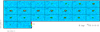 |
Fig. 2 ALMA maps per velocity channel of 12CO J = 3−2 emission in R Aqr obtained with a more compact ALMA configuration; see the LSR velocities in the upper left corners. The center is the centroid of the continuum, whose image has been subtracted. The contours are logarithmic, with a large jump of a factor 2 and a first level of ± 5 mJy beam−1 (equal to 3.4 times the rms and equivalent to 2.06 K). The dashed contours represent negative values. The HPBW is shown in the inset in the last panel. The represented field is wider than in our other maps. |
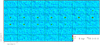 |
Fig. 3 ALMA maps per velocity channel of 13CO J = 3−2 emission in R Aqr (only the more extended array configuration); see the LSR velocities in the upper left corners. The center is the centroid of the continuum, whose image has been subtracted. The logarithmic contours and scales are the same as in Fig. 1 (in this case, the first contour, 5 mJy beam−1, is equivalentto 5.6 times the rms and 35.2 K). The HPBW is shown in the inset in the last panel. |
 |
Fig. 4 ALMA maps per velocity channel of 12CO J = 2−1 emission in R Aqr; see the LSR velocities in the upper left corners, similar to Fig. 1. The contours are logarithmic, with a jump of a factor 2 and a first level of 4 mJy beam−1, equivalent to 4.9 rms and 11.33 K. The dashed contours represent negative values. The HPBW is shown in the inset in the last panel. |
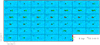 |
Fig. 5 ALMA maps per velocity channel of 12CO J = 6−5 emission in R Aqr; seethe LSR velocities in the upper left corners. The contours are logarithmic, with a jump of a factor 2 and a first level of 50 mJy beam−1, equivalent to 3.6 times the rms and 41.5 K. The dashed contours represent negative values. The HPBW is shown in the inset in the last panel. The velocity channels are the same as in Fig. 1, but the represented field is larger. The image center is the centroid of the continuum, whose image has not been subtracted (Sect. 2). |
3 Observational results: molecular line maps
We presenthigh-quality ALMA maps of 12CO J = 2−1, J = 3−2, and J = 6−5 and of 13CO J = 3−2, see Figs. 1 to 5 and Sect. 2. Observations of other lines and the adjacent continuum are presented in Bujarrabal et al. (2018) and Gómez-Garrido et al. (in prep.).
In Fig. 1, we show our high-resolution J = 3−2 maps that were before discussed in Bujarrabal et al. (2018), after a reanalysis that included rebinning of the velocity channels. Figure 2 presents maps obtained with a more compact configuration, which yields a somewhat poorer resolution but higher brightness sensitivity. The emission structure is better described in Fig. 1, but the data in Fig. 2 confirm the detection of very weak clumps (tentatively detected in the high-resolution maps) at offsets (Δα,Δδ) ~ (0.6,−0.2) and (− 0.9,−0.2) arcsec. There is also a closer component at approximately (− 0.3,0.1), which is somewhat wider and appears in a larger velocity range, between − 23 and − 12 km s−1 LSR. These clumps, particularly the last one, are also clearly detected in 12CO J = 6−5, see below.
Figure 4 shows observations of 12CO J = 2−1, obtained after merging observations with two different configurations. The brightness distribution is quite similar to that of J = 3−2, but weaker, as expected because of the difference in frequency and opacity. Precisely this difference in opacity is of particular interest in our modeling (Sect. 4).
Finally, we show our 12CO J = 6−5 maps in Fig. 5. The weak sparse clumps mentioned above are better detected in this line, probably because of its higher opacity, which decreases the contrast between high- and low-density regions. The higher opacity and excitation requirements of this line are also useful in modeling the CO emission. The represented field is larger in this figure than for Fig. 1 in order to show the weak clump emission.
Some straightforward results can be directly extracted from our maps of molecular line emission in R Aqr. We list them below.
12CO J = 3−2, J = 2−1, and J = 6−5 lines are resolved in our ALMA maps. They occupy a region of about 0.7 × 0.2 arcsec (elongated more or less in the east-west direction). A few sparse, very weak spots are detected at distances between 0.″ 5 and 1″. Despite the high sensitivity of our ALMA maps (we reach very high signal-to-noise ratios, S∕N > 100 in most maps),these clumps are barely detected.
Both single-dish (Bujarrabal et al. 2010) and interferometric data indicate relatively weak total (angle-integrated) fluxes, for instance, Fpeak(J = 2−1) ~ 0.2 Jy. The single-dish and angle-integrated ALMA profiles are very similar (Sect. 2). The 12CO line intensities are far lower and the extents are far smaller than for standard AGB stars. For the same mass-loss rate and distance (>10−7 M⊙ yr−1, ~ 265 pc), we would expect 12CO J = 2−1 peak fluxes >10 Jy and extents >10″ (e.g., Castro-Carrizo et al. 2010). The CO lines in standard AGB sources are about a hundred times more intense and extended than in R Aqr.
Except for the 12CO lines, the emissionof all other molecules in R Aqr is very compact (Bujarrabal et al. 2018; Gómez-Garrido et al., in prep.) and still much weaker. Most lines occupy less than 0.″ 1 and even 13CO lines are more compact than 0.″ 2. In standard AGB envelopes, molecules other than 12CO show sizeable extents >1″ (see, e.g., Agúndez et al. 2017; Verbena et al. 2019). The extent of 13CO is often almost comparable to that of 12CO in AGBs because the lower degree of selfshielding of 13CO to the interstellar UV is partially compensated for by fractionation reactions (Cernicharo et al. 2015; Mamon et al. 1987, etc).
The 12CO line maps show a central condensation, plus some plumes that mostly extend in the east–west direction. The condensation is 0.″1-0.″ 2 wide. It is centered on the expected position of the AGB star and slightly exceeds the full orbital region (the typical angular separation between the two stars is up to ~50 mas, see Sect. 1).
In all three 12CO lines, the extended plumes appear to be part of a spiral structure that is mostly confined to the orbital plane and is seen almost edge-on (as was mentioned by Bujarrabal et al. 2018, this is more widely discussed in Sect. 4). The complex velocity structure suggests a complex dynamics that probably includes both tangential and radial expansion movements.
The different observations were obtained at different epochs, and because we were close to a tight periastron (that took place at the end of 2019), fast variations in the relative stellar positions are expected. In any case, all 12CO maps show quite comparable distributions.
The fact that the J = 6−5 line is the most intense confirms that the lines come from high-excitation regions, with temperatures that exceed its excitation energy (EJ = 6 = 115 K), and densities that are high enough to significantly populate these levels despite its high A-coefficient (2 × 10⁻⁵ s−1), n ≳ 106 cm−3. The brightness peak in K-units, ~550 K, implies gas temperatures higher than this value in the central regions. In addition, because the typical gas temperatures in the inner circumstellar envelopes are usually not very high, about 1000 K at most, the opacity in this line must be ≳1 in the central regions and somewhat lower elsewhere.
In general, the dependence of the brightness level on the line strength shows that the lines are not opaque: J = 2−1 reaches a peak brightness of 250 K, while J = 3−2 is intermediate between J = 2−1 and J = 6−5. We conclude that optical depths must be moderate, depending on the line and analyzed component, with opacities between lower than 0.25 and ~2. Our modeling (Sect. 4) confirms this result.
Our observations of 13CO J = 3−2 (Fig. 3) confirm a significant opacity of the 12CO line in the central regions because the 12CO/13CO line ratio is low (~3), but not in the outer regions, in which practically no 13CO emission is detected.In any case, the abundance ratio must be low (~ 10–15), in view of the expected values of the opacities and the moderate line intensity ratio. We also note that the maps, with slightly resolved emission from this central clump, show a very simple structure that is not compatible with a significant rotation, but suggest simple expansion at moderate velocities ≲ 10 km s−1.
It is important to realize the strong difference between the brightness distributions observed in R Aqr and those typical of standard AGB stars (see, e.g., Castro-Carrizo et al. 2010; Cernicharo et al. 2015; Guélin et al. 2018; Homan et al. 2018; Decin et al. 2020), which were obtained using similar observational techniques. In most cases, the circumstellar envelopes seem to be composed of more or less complete spiral arms or arcs, which are probably the result of interaction with a low-mass companion, but the overall structure is spherical and the kinematics is roughly isotropic expansion. Only in some objects, such as the semiregular variables R Dor and X Her, does the circumstellar envelope show an hourglass-like structure with a clear symmetry axis. These peculiar objects appear in some way to be intermediate between the usual roughly spherical shells and the nebula around R Aqr.
4 Modeling the ALMA maps of R Aqr
As described in Sect. 3 and Bujarrabal et al. (2018), a first inspection of the ALMA maps strongly suggests that the CO line emission comes from spiral arcs that are strongly focused on an equatorial plane and are seen roughly edge-on. This might be compatible with results from hydrodynamical calculations and the expected geometry of the binary orbit and circumstellar shells in R Aqr (Sect. 1). The amount of information included in our high-quality maps allows a more detailed comparison with predictions from the hydrodynamics of the system. For this purpose, we performed an heuristic modeling of the data in order to describe the main properties of the CO-rich detected nebula (see Sect. 4.1), as well as hydrodynamical models of the gravitational interaction between the WD companion and the AGB wind for the case of the R Aqr system (Sect. 4.2).
From our first attempts to model the ALMA observations, we readily found that the predictions from hydrodynamical models by themselves are not able to provide an adequate density distribution, as they are in general too extended to explain the small emitting region and the very weak total CO emission. The very weak single-dish CO lines already require a very limited emitting region, see Sect. 3 and Bujarrabal et al. (2010), instead of spiral arms occupying extended regions (more than 10″ wide) that are globally similar to a standard AGB circumstellar envelope. In addition, the ALMA maps only show a clearly defined and limited group of spiral arcs, just some threads of the inner spirals. Our simplified descriptive model of the CO-emitting region (Sect. 4.1), based on the general properties of the hydrodynamical predictions, is devoted to describing the maps in terms of the emission of some inner arcs, as well as to defining the properties that they must satisfy to reproduce the observations. We further conducted new hydrodynamical calculations for the case of R Aqr (Sect. 4.2), including in particular the effects of its significantly eccentric orbit. The comparison between the descriptive and hydrodynamical models will allow us to improve our understanding of the effects of gravitational interaction between the compact companion and the inner circumstellar shells.
Finally, we also try to understand the molecule photodissociation due to the strong UV field of the white dwarf star. We show below (Sect. 4.3) that photodissociation can be strongly selective and might explain that only some pieces of the spiral structure show molecular emission. We stress the extremely difficult treatment of the chemistry in our source, which has a very complex structure and dynamics and a significant variation with time (because the orbital period is comparable to the abundance evolution times in many cases).
The goal of this modeling effort is to allow a sensible comparison between the observations and the hydrodynamical simulations of the strong gravitational attraction effects of the WD on the AGB wind. Because the observations just probe the CO-rich regions, which are probably affected by photodissociation, the chemistry induced by the UV radiation of the WD must be also accounted for. In any case, the results of our heuristic model, as they are basically a description of the emitting region responsible for the maps, are actually closer to the CO-rich gas distribution than any result from hydrodynamical and chemical calculations, which are quite a-prioristic and mainly useful for understanding the origin and meaning of the detected features.
4.1 Descriptive, heuristic modeling of the CO line emission from R Aqr
4.1.1 Main model characteristics and nebular components
As mentioned, direct calculations of CO emission using predictions directly from hydrodynamical models cannot explain some obvious properties of the CO emission. In addition, a long iteration of hydrodynamical calculations plus CO line emission simulations plus a comparison with maps plus hydrodynamical calculations, etc., is not feasible because hydrodynamical modeling is delicate and time-consuming. Accordingly, we developed a descriptive model of the CO-emitting region that accounts for the general properties of the hydrodynamical predictions and the expected photodissociation effects. This model describes the properties that the CO-rich gas distribution and kinematics must show to reproduce the observations. These properties are finally discussed based on theoretical considerations.
The code we used for our heuristic model allows general 3D distributions of the physical conditions and kinematics, whose descriptions are quite free. Gas velocities can show both radial (expansion or infall, though we favor expansion movements) and rotational (i.e., tangential) components. The contrast between equatorial and adjacent regions could be very sharp and high, the spiral arcs can be more or less complete, etc. The only basic assumptions or “axioms” we adopt in our modeling are that there is a symmetry plane (the equator), which is the same as that of the orbit, and that the gravitational interaction can induce in the gas a tangential velocity in the direction of the movement of the companion, both expected from theoretical descriptions of interaction in SSs, as summarized in Sect. 1. We also take previous empirical information on the orbit (Sect. 1) into account, notably that the axis of the orbit is almost in the plane of the sky, that its north pole is slightly tilted to the east and pointing to us, and that the secondary was moving toward the observer during the observing runs.
To reproduce the general features of the CO maps (Sect. 3), our model must assume, more specifically, that the emissioncomes from the inner circumstellar envelope, whose general structure consists of a central condensation, occupying a region with a size comparable to the orbit and responsible for the central clump detected in the maps, and a series of discontinuous spiral arcs that are strongly focused on the equatorial plane and are responsible for the plumes detected around the central clump. The remaining envelope, including the interarms and regions far from the equator, must contain a very low density of CO molecules (as indicated by the observations, Sect. 3).
The central condensation is only poorly resolved by our mapping. Therefore its structure is not described in detail in the model and we discuss only global properties, even if this can be very complex (as shown in Sect. 4.2). We just assumed the same kinematics as in a standard inner AGB shell, with a moderate outward velocity that increases with the distance. It is remarkable that the observations do not show any sign of rotation in these inner regions. This is particularly the case of 13CO J = 3−2 (Fig. 3), which comes only from this region and in which no shift in velocity between the west and east parts of the clump is found.
Hydrodynamical calculations suggest that the spiral arcs first include a spiral arm leaving the central condensation, approximately from the place at which the WD star is expected, and developing counterclockwise. These CO-rich spiral arcs in our model also include the threads of outer spiral(s) that are still CO-rich. The gas velocity in the arcs must be a composition of tangential and radial velocities.
The line excitation is described in the code by LTE. This is fully justified for our low-J transitions (with relatively low A-coefficients) and under the expected conditions in the inner circumstellar regions, with high densities ≳106 cm−3 (see, e.g., Bujarrabal et al. 2010 and the discussion in Appendix A). With all these ingredients, we calculated the brightness distribution for very many lines of sight (i.e., angular offsets with respect to the nominal center) and velocity shifts (i.e., frequencies corresponding to Doppler shifts for different LSR velocities) by solving the standard radiative transfer equation. This distribution is numerically convolved with the observational beam, yielding maps that are directly comparable to the ALMA maps (as they show little flux loss). The code is similar to that we used in previous studies (e.g., Bujarrabal et al. 2016, but we assumed no axial symmetry here). With this treatment, the calculations are relatively fast. The full calculation required some seconds with a PC in standard runs and one or two minutes for the most accurate calculations.
The model predictions were compared with the ALMA maps. We considered for this purpose the high-quality 12CO J = 3−2 maps (Fig. 1), which show an extended distribution. We also compared with other CO maps, but less in detail because their quality is lower and they were obtained at different epochs (as mentioned, Sect. 3, comparing data from different epochs in such a rapidly evolving system is not straightforward). We show in Fig. 6 (top) the density and velocity distributions of one of the best-fit models in the equatorial plane (i.e., the z = 0 plane in our frame). The y = 0 and x = 0 planes are also represented in Fig. 6. In this best-fit model we also take an angle between the equatorial plane and the line of sight of 15° and a position angle of the rotation axis projection on the plane of the sky of 5°. In Fig. 7, we show the 12CO J = 3−2 maps predicted by this nebula model, to be compared with observational data (Fig. 1; the units and scales are the same in both images). The comparison is very satisfactory. The correspondence between the different components in our model and the predicted features (and corresponding observed features) is very direct, see the next sub-subsection, showing that there is not much room for changes in the proposed CO-rich gas distribution and kinematics.
We clearly identify several components in the model. We include the central condensation, component A in Fig. 8, plus spiral arcs. These are composed of an inner arc close to the WD (component B), its outer parts (component C), an intermediate small arc (D), and a weak outer arc (W). Other still fainter clumps (W′) are also considered to explain some more distant, poorly mapped features. ? represents the strong feature detected at −26 km s−1 LSR, at about 0.″ 1 northeast, whose origin is not easily understood in terms of the expected dynamical components. W′ and ? are in fact not included in our modeling (Fig. 6) and are not discussed in depth.
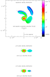 |
Fig. 6 Top: density distribution of the CO-rich gas in the plane of the equator (z = 0 plane in our coordinates) from our best-fit model. Equatorial velocities are also represented. Middle: density distribution in the y = 0 plane and velocities projected in that plane. Bottom: same, but for the x = 0 plane. All representations share the same units and scales. |
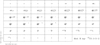 |
Fig. 7 Predictions of our best-fit heuristic model for the 12CO J = 3−2 line maps, to be compared with observations, Fig. 1. All units and scales are the same as in Fig. 1. |
4.1.2 Correspondence between the main components of the model and the observed features
To better understand the meaning of the various model components, we also show in Fig. 8 (bottom) a view of the equatorial density distribution seen from a certain inclination of the equator with respect to the line of sight. This representation is only illustrative because, to avoid confusion, we only accounted for the equatorial density. We also represent the projection of the gas velocity in the line-of-sight direction. We again stress that this is just an approximation because only the equatorial regions and velocities are considered, but we recall that the density and acceleration due to the WD attraction are assumed to be high only very close to the plane.
The regions in which the gas recedes from us (vectors pointing upward in Fig. 8) must correspond to observed features in the maps with relatively positive velocities. When the gas approaches us (vectors pointing downward), the emission must be detected at relatively negative velocities. Because all the nebula shares the characteristic circumstellar expansion in some way, regionsplaced behind the star should tend to emit at positive velocities. The rotation introduced by the gravitational interaction should yield negative velocities for nebular regions placed close to the WD (which is placed slightly rightward in our representation and approached us during the observing run). We mentioned that both expansion and rotation are accounted for in our model.
In Fig. 9, we show maps for representative velocity channels, in which the correspondence between the observed features andthe above components is indicated. The central condensation must show both positive and negative (moderate) projected velocities as a result of the expansion previous to interaction with the WD. Component A in Fig. 8 can therefore explain the observed central condensation with a moderate velocity dispersion around the central one (feature A in Fig. 9); note that the meaning of central velocity in our case is not obvious, the velocity of the system barycenter is ~ − 24.5 km s−1 LSR (Alcolea et al., in prep.), but the AGB star showed a slightly more positive velocity during the observations. In component B, the expansion projection is almost negligible and the rotation is expected to be high. These components explain the negative-velocity feature (B in Fig. 9). It is possible that both expansion and rotation contribute to explain the negative velocity in D. In the outer regions of the spiral arm, C, the projected velocity is dominated by the expansion, and it is responsible for the arc that is clearly detected at relatively positive velocities. Finally, we introduced diffuse outer arcs W, W′. W can explain the sparse very weak clumps detected in the outer regions at northwest offsets. W′ vaguely represents two of the weak southern clumps detected in the low-resolution maps (Fig. 2). These components probably are remains of the very outer regions of the B–C arm (see a tentative general view in Fig. 14). W′ was not included in our modeling because their nature was too uncertain. We recall again that these weak components may show a clumpy emission pattern that is not clearly defined in our data.
In our maps, we also identify a conspicuous feature that cannot fit the general features of our modeling, see label ? in Figs. 8, 9. If it is equatorial, this component should be placed behind the star, but it shows a negative velocity projection, which cannot be explained by our model (with just expansion and rotation velocities). We suggest that it is the result of the emission of a CO-rich gas clump falling back to the AGB star and is perhaps not exactly placed on the equator, which would remain CO-rich because of shielding by the AGB star surroundings. Inflows due to complex hydrodynamical interactions are sometimes predicted by model calculations, mostly in off-equator regions (see Sect. 4.2), but the description of their very complex structure and dynamics is beyond the scope of our simple modeling, and we only point out its existence.
We stress that some quantitative results in our descriptive modeling are necessary to explain the observations, provided that the general assumptions (our “axioms” described above) are true. We list those results below.
The general structure of the CO-rich gas in our model, with the central condensation and several arcs placed close to the equator, is necessary provided that we assume equatorial symmetry and that we know with reasonable accuracy the inclinations with respectto the north and to the line of sight. The observed features directly correspond to those of the model, and more extended CO-rich gas is improbable.
The sizes of the model components are also necessary, within the (very good) angular resolution of our observations, scaled for the value of the distance (which gives the conversion from angular to linear units), and depending on other assumptions. For instance, the size of the central clump, component A, must be of about 7 × 1014 cm; the uncertainty, ~2 × 1014 cm, due to the resolution and to the contribution of nearby components, is not negligible. The contribution of other components is also the main source of uncertainty for the shape and extent of B; they must be accurate if the identification scheme depicted in Fig. 9 is correct. The outermost arcs (D and W) must reach a distance ~ 1.5 × 1015 cm, which is an accurate estimate: the most distant emission in Fig. 1 reaches ~ 0.″ 4 and, because of its low declination offset, these regions must be placed roughly perpendicular to the line of sight. The outer part of the first arm (component C) must be placed at ~ 7 × 1014 cm. This value depends on the adopted inclination with respect to the line of sight. For an inclination of 30°, the distance to C would be twice smaller, and C would be 1.5 times farther for inclinations of about 10 degrees. Out of this range (already generously wide), C could not be considered as a continuation of B.
Some properties of the velocity field in our model are also necessary to describe the observations. The expansion velocity of the central clump is directly given by the dispersion of the central intense feature in the maps, within 1 km s−1. The expansion velocity of component C is accurately given by the shift in velocity of the corresponding observed feature, 10–15 km s−1; however, its rotational velocity, which points more or less perpendicularly to the line of sight, is only poorly determined. In contrast, the rotational velocities of components B and D, which basically point to us, are accurately determined and must be of 3–10 km s−1 to explain the observed blueshifts. Expansion velocities in W of about 5–9 km s−1 (with low rotation) are also necessary, although in this case, the weak detected emission and the high angles between thevelocity and line-of-sight vectors may significantly affect our estimates. All these velocities depend slightly on the inclination of the equator with respect to the line of sight (provided that it is ≲ 30°) because all components are basically placed in the equator. It is important to note that some of the kinematical items of our description show a certain degree of degeneracy. Rotational and radial velocities could change in some areas, notably B and D, provided that the projected velocity in the direction of the observer is kept the same. Component D could be slightly shifted to positive values of the y-axis in Fig. 6, partially occupying the region between B and W; then we would have to introduce a higher rotation velocity that is hardly compatible with the hydrodynamical calculations in Sect. 4.2 (although we would achieve a better fit of the observed maps). In these cases, we generally tried to adapt our heuristic model to the results obtained from hydrodynamical calculations.
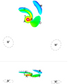 |
Fig. 8 Top: main components identified in our simple model (see Sect. 4.1). Bottom (below the dotted line): Representative image of the equatorial density distribution as seen with the actual inclination of the equator. This image is a very simplified representation to facilitate interpretation, in which the latitude density distribution is not accounted for. The projection of the equatorial velocity in the direction to the observer is also represented (directly taken from the velocity vectors in Fig. 6, top). Again this is only illustrative because the off-equator movements are not considered. Downward arrows represent gas approaching the observer (relatively negative LSR velocities), while arrows pointing upward mean that the gas recedes from us (relatively positive LSR velocities). |
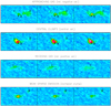 |
Fig. 9 Representation of the different observed features (from Fig. 1) and the components of our model (A, B, C, D, W, and ? in Fig. 8) that are responsible for the corresponding predicted emission. |
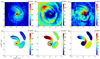 |
Fig. 10 Top: hydrodynamical model versus (bottom) our heuristic model for (a, d) number density, (b, e) radial velocity, and (c, f) rotational velocity distributions of the gas in the equatorial plane. Color bars label in units of cm−3 for number density and km s−1 for velocities.The overlaid arrows represent the gas velocity vectors. The pericenter of WD is located on the straight white line, and the current orbital phase of the binary stars is at 65° before the pericenter. |
4.2 Hydrodynamical simulations of the interaction between the compact companion and the AGB wind. Comparison with our heuristic model
We performed hydrodynamical simulations with the stellar and orbital parameters of R Aqr binary stars using the code FLASH 4.5 (Fryxell et al. 2000). The fluid motion is governed by the continuity, momentum, and energy equations for hydrodynamics, including the gravitational attraction toward the individual stars, and the intrinsic acceleration of AGB wind mimicking radiation pressure onto dust particles (for details, see, e.g., Kim et al. 2013, 2019). We also implemented radiative cooling of the gas and accretion sink onto the white dwarf (Lee et al., in prep.).
In the simulations, we adopted the AGB and WD masses of 1.41 M⊙ and 0.82 M⊙, respectively,and the average orbital separation (sum of the semimajor axes) of 15.7 AU, yielding an orbital period of 42 yr. The mass-loss rate of the AGB star was adopted to be 3 × 10⁻⁶ M⊙ yr −1. An orbital eccentricity of 0.57 was applied, causing the orbital separation to vary from 24.6 AU at the apocenter down to 6.8 AU at the pericenter. The orbital velocity of the WD varied from 3.7 km s−1 at the apocenter to 13.5 km s−1 at the pericenter, which is comparable to the expansion velocity of the AGB wind. The sufficiently fast orbital velocity relative to the radial wind velocity causes the “transverse” velocity component in the flow near the WD near its pericenter, while the flow tends to pass the WD straight at its apocenter. As a consequence, the flow near the stars becomes very complex over the entire orbital phase. Although some hydrodynamic simulations in the literature treated highly eccentric orbit cases such as e = 0.8 (e.g., Kim et al. 2017, 2019; Randall et al. 2020), their lagging stellar orbital velocities made the situation relatively simpler than the model visualized here.
We iterated hydrodynamic simulations to examine the wind velocity acceleration with the fixed stellar and orbital parameters. The wind velocity near the stars (in particular, the velocity near the WD) controls the formation of the accretion disk, the portion of wind escaping from the gravitational potential of stars, and the overall shape of the spiral (see details in Lee et al., in prep.). The situation becomes more complicated when the orbital shape is noncircular: the spiral pattern is then pushed out faster at the pericenter and relatively more slowly at the apocenter.
Our basic nebula description (Sect. 4.1) is quite similar to some of the hydrodynamical predictions, see Fig. 10, but in our descriptive model only some parts of the spiral structure appear and the contrast between them and the surrounding regions is stronger. We attribute these differences to the selective photodissociation of CO by the WD UV field, see the discussion in Sect. 4.3.
The main features of the hydrodynamical model exhibited in Fig. 10 are listed below.
For the A, B, C, D, and W components defined in Sect. 4.1, their locations and density levels match the dense structures in the equatorial plane in the outcome of the hydrodynamical simulation reasonably well. The significant drop in spiral density following the C region is of particular interest. It is consistent with the ALMA images showing a relatively small extension toward the east.
Component B, indicating the spiral arm at high density attached to the WD, is clearly identified in our hydrodynamical model. At the head of the spiral in this model, the flow mostly shows a rotational motion in the clockwise direction with the velocity of 11–13 km s−1 on average within the scale height of ~5 AU. In the immediate neighborhood of the WD, the rotational velocity of the flow increases to 28 km s−1.
The spiral tail following the WD is well located within the C region defined in the heuristic model. The expansion velocity of this spiral pattern is up to 11 km s−1, which is slightly lower than the velocity criteria in Sect. 4.1. However, the three-dimensional data cube of the hydrodynamical model shows that, above the equatorial plane, the spiral pattern shifts toward the + y direction, which would be degenerate in the observation of the R Aqr binary system as the orbit is viewed close to but not exactly edge-on. The expansion velocity of this spiral-shell pattern approaches 12 km s−1, with some variations along its vertical stretch from the equatorial plane (see Fig. 11b).
The abrupt density decrease beyond the B–C spiral arm, which appears in both the observations and the hydrodynamical calculations, is probably due to the high eccentricity of the orbit. A circular-orbit simulation, which was tested with the same orbital parameters except for the orbital shape, does not show this density discontinuity. In general, it exhibits smooth undulations that extend in a highly isotropic manner, which contradicts the observed pattern.
The D region shows the convergence and divergence of many different branches of density flows caused by various velocity components due to the initial AGB wind acceleration process, the effects from eccentric orbital motions of the stars, and some fallback flows toward the equatorial plane. The net expansion and rotational velocities of the flows within region D are not higher than 6.5 and 4.5 km s−1, respectively, in agreement with our descriptive model.
The arc appearing in region W has a shell structure with an expansion velocity up to 6.5 km s−1 considering a typical height of 15 AU. The rotational velocity is low and does not exceed 2 km s−1.
Finally, we stress the presence of some infall toward the AGB star (Fig. 11; notably from the other side of the WD). As discussed in Sect. 4.1, this feature may qualitatively explain the observed component ?, which is otherwise very difficult to understand, provided that some of the infalling gas remains CO-rich.
In order to mimic the observing view for the nebulae around the R Aqr binary system, independently of the comparison with the heuristic modeling, we rotated the hydrodynamical model cube about the x-axis until the equatorial plane is at 15° from the line of sight. The WD approached us and was located in the southern part. Fig. 12 shows the column-density channel maps of our hydrodynamical model at six representative velocities. In general, the channels near the systemic velocity show superfluous features compared to the ALMA maps per velocity channel, which would be mostly invisible in CO line transitions due to photodissociation (see Sect. 4.3). Nevertheless, we can obtain some useful information from this simulation by comparing with the ALMA channel maps, in particular, for the relatively less-structured channels at high velocities. We found that the expansion velocity of component C is up to 10 km s−1 (with respect to the systemic velocity) in the equatorial plane, but increases to 12 km s−1 at its vertical stretch in the off-plane. This component is apparent in the channel map at 12 km s−1 with respect to the systemic velocity as a nearly horizontal feature to the northeast. It corresponds to the emission in the ALMA channel maps at the LSR velocities of −14.2 to − 10.2 km s−1 (see Fig. 1). The column-density channel map at − 8 km s−1 shows the enhanced density distribution to the southwest 0.′′2, while the corresponding ALMA map (LSR velocities near −31.8 km s−1) is extended mostly to the west up to 0.′′3. We also have an indication for the ? component from the north-northeast stretch in the − 4 km s−1 column-density map (top panel). Its disappearance in the bottom panel might further imply a survival of this dense gas cloud at some height from the equator against the photodissociation effect described in Sect. 4.3. Finally, in Fig. 13, we show a position-velocity diagram of column density along the east-west central cut with the width of the slice corresponding to the beam size of 12CO 3–2 maps. Fig. 13 displays the asymmetric velocity distribution in the redshift to the east up to ~ + 11 km s−1 (component C) compared to the blueshift up to ~ − 7 km s−1 (D). The very large velocity dispersion of component B is also clearly visible.
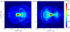 |
Fig. 11 Density distribution of the gas in the hydrodynamical model in the (a) y = 0 and (b) x = 0 planes, revealing the vertical flattening onto the equatorial plane. The velocity vectors show the fallback of gas toward the equatorial plane and the AGB star from up to the height of 50 AU. |
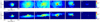 |
Fig. 12 Top: column-density channel maps of our hydrodynamical model at an inclination of 15° from the edge-on view of the equatorial plane, and (bottom) the same, but with a pseudo-restriction of the density distributionup to a height of 15 AU. The central velocity of each channel with respect to the systemic velocity (~ − 24.5 km s−1 LSR) is indicated at the top left corner of each panel, and the individual channel width is 4 km s−1. Color bars are in units of g cm−2 (km s−1)−1. |
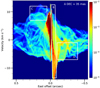 |
Fig. 13 Position-velocity diagram of our hydrodynamical model at an inclination of 15° from the edge-on view of the equator. The velocity is measured with respect to the systemic velocity. The color bar is in units of g cm−2 (km s−1)−1. See observations in Bujarrabal et al. (2018). |
4.3 Effects of photodissociation on the extent and shape of the CO-rich region
Except for H2, CO is the most abundant molecule in circumstellar envelopes around AGB stars and shows the largest extent because it is very efficiently selfshielded against interstellar UV radiation (Mamon et al. 1987; Cernicharo et al. 2015). A strong emitter of UV radiation in the hot and dense inner regions of the envelope, as it is the case of the white dwarf in the R Aqr symbiotic stellar system, might induce important changes on the distribution of CO, compared with standard AGB envelopes. The first important effect is related to the morphology of the whole gaseous and dusty envelope, as a consequence of the gravitational interaction with the white dwarf (see Sects. 3 and 4.2). The second important effect is related to the photodissociation induced by UV photons emitted by the white dwarf, which can affect the distribution of molecules, including CO, within the envelope.
As mentioned (Sect. 1), the properties of compact companion are difficult to determine. In addition, we must realize that the derived parameters mostly refer to the emission of the WD and its surroundings, including the probable accretion disk. The radiation parameters of the UV source were discussed by Kaler (1981), Burgarella et al. (1992), Meier & Kafatos (1995), and Schmid et al. (2017). Their estimates of the temperature range from ≈ 40–80 kK, and for the luminosity from ≈0.05 L⊙ to 5–20 L⊙. For the purpose of this study, we therefore decided to make our own estimates. We used two long-exposure IUE spectra of the central source of R Aqr taken on 14 July 1991 (SWP 42 069 and SWP 42 070). The coadded spectra revealed a rising continuum for λ≲1700 Å, while the equivalent width of HeII 1640 emission line, EW(1640) = 9.9 ± 1.3 Å, is consistent with an ionizing source with an effective temperature T ~70 000 K. In this analysis, we assumed a typical reddening E(B − V)~ 0.23 mag along the line of sight toward the WD, which is somewhat lower than the average values found toward the Mira (Sect. 1), according to results usually found in SSs (see Mikolajewska et al. 1999; Gromadzki et al. 2009). We note that a significantly higher extinction toward the WD is also incompatible with the appearance of the IUE spectrum. Assuming a blackbody distribution of the hot WD continuum, we fit the R-J tail to selected continuum windows shortward of λ ~ 1700 Å. The best fit to the UV continuum and HeII 1640 emission line flux was obtained for T ~ 80 kK and RWD∕d ~ 1.1 × 10⁻¹², which, assuming a distance of 265 pc, gives L ~ 6L⊙. The radius of the hot WD is consistent with a CO WD radius with a mass of ~ 0.7–0.8 M⊙ (compatible with our orbital solution). Similarly, we derived T ~ 70 kK and L ~ 4.5 L⊙ from the coadded IUE spectra taken in 1980–1986. Accordingly, we finally adopt T = 80 000 K and L = 5 L⊙ as representative values to be used for analyzing the effects on molecular photodissociation.
In regard to photodissociation, we expect that the UV photons emitted by the white dwarf first create a relatively compact HII region around it, where UV photons with energies higher than 13.6 eV are fully absorbed, and a second region located farther away, showing the typical stratification C+ /C/CO of dense photon-dominated regions (PDRs; Tielens & Hollenbach 1985). That is, we could expect a more or less spherical region void of CO around the white dwarf. Depending on various key parameters, such as the mass-loss rate of the AGB star, the separation between AGB and WD, and the effective temperature and luminosity of the WD, the effect on the CO distribution can be very different. It ranges from a small CO-depleted region around the white dwarf, which may be difficult to probe through observations, to a strong effect on the CO envelope, leading to complex morphologies or even to a complete removal of the CO envelope in certain SSs.
Modeling the photodissociation of CO in such a system becomes challenging because of several complications. One of them is that the spherical shape of the envelope can be strongly distorted by the gravitational effect of the WD, leading to complex spiral-like structures and a complicated kinematics in which expansion and rotation are mixed. The relative abundance of dust is highly uncertain in the surroundings of the AGB star because dust is expected to form at a certain distance from the red giant. Moreover, the orbital timescales can be comparable to the (photo)chemical timescales, creating a time-dependent problem in which the shape of the CO-rich envelope can vary with time.
When we take the high prevalence of binary stellar systems into account, interest in modeling the effect of internal UV sources in AGB envelopes is timely (e.g., Saberi et al. 2019), although for the moment, models cannot solve the complications described above. We evaluated the effects of UV radiation from the WD on the distribution of CO in the R Aqr system by using the Meudon PDR code (Le Petit et al. 2006), in which we implemented a correction to take the geometrical dilution of the UV field (and of photodissociation rates) with increasing distance from the WD into account. We evaluated the chemical composition at steady statealong four representative directions from the white dwarf lying in the orbital plane (at longitudes Λ = 0°, 90°, 180°, and 270°, where Λ = 0° corresponds to the direction toward the AGB star and the angles increase counterclockwise; see Fig. 14). We adopted an extended version of our heuristic model (Sect. 4.1), in which we crudely extended the description of the density distribution also to regions that, presumably because of photodissociation of carbon monoxide, are in fact not observed in CO lines. We therefore recall that, because of the lack of empirical information and the complex structure suggested in the hydrodynamical models, this extension is very tentative. We also explored models in which we decreased the density by factors of two and three because the determination of the column densities of gas and dust from our line emission fitting is relatively uncertain: it depends significantly on various parameters, such as the fractional abundance of CO, the conversion from gas to dust densities, and the actual velocity dispersion. We adopted solar elemental abundances and the gas-phase chemical network used by Agúndez et al. (2018) to model protoplanetary disks, which also host dense, warm, and UV-illuminated regions, as in R Aqr. Optical and infrared observations of Mira-type (O-rich) AGB stars have shown that the most relevant elements (C, N, and O) have essentially solar abundances (e.g., Smith & Lambert 1986; Gałan et al. 2017). Elemental abundances have not been determined in symbiotic systems with a Mira star, such as R Aqr, but we can reasonably expect that elemental abundances would not deviate much from solar. Moderate deviations would not affect the main conclusions obtained from the PDR models, although they may slightly hinder the comparison between total column densities in our heuristic model and in chemical models.
We considered dust extinction typical of the interstellar medium, but with a dust-to-gas mass ratio half of the interstellar value to account for the probable depletion of dust in the surroundings of the AGB star, where dust has not yet fully formed. The kinematics of the envelope is complex, and this might reduce the selfshielding of CO. Because the Meudon PDR code does not allow treating velocity gradients, we adopted a relatively high turbulent velocity of 15 km s−1 to reduce the optical depth of the UV lines of CO and the extent of selfshielding.
For the conditions adopted here to model the photodissociation of CO in R Aqr, we find that the C+ /CO transition lies at a visual extinction of about 2 mag from the WD. In the extended heuristic model (panels on the rightin Fig. 15), the adopted densities result in total visual extinctions higher than ~ 5 mag for any direction in the orbital plane, implying that the C+/CO transition lies close to the WD and that beyond this point, CO is very abundant regardless of the longitude (see panel b on the right in Fig. 15). In the direction toward the AGB star, at Λ = 0°, CO is depleted at distances between 1.5 × 1014 cm and 8 × 1014 cm (see panel c on the right in Fig. 15), however, because CH4 becomes themain C-bearing molecule. This fact is predicted by the chemical model for a very concrete region of R Aqr (inner shells on theother side of the WD) as a consequence of the lack of UV and high temperatures prevailing there (500–1000 K). It has been also predicted to occur in dense, warm, and UV-illuminated regions of protoplanetary disks (Agúndez et al. 2008). It is difficult to verify a phenomenon like this in our case because of the complex CO-emission structure, but we do not find any clear sign of strong CO depletion in the close surroundings of the primary (CO is also found to be abundant in the inner shells around standard AGB stars). This feature arises in the model because chemical reactions tend to incorporate carbon into CH4 rather than into CO at high temperatures. In R Aqr, however, CO is expected to be formed in the close surroundings of the AGB star in thermochemical equilibrium conditions, and, if sufficiently shielded from the UV radiation, the possibility is low that it is dissociated to liberate atomic carbon and to allow chemical reactions to convert it into CH4 in times shorter than the system evolution time. We therefore consider that the displacement of CO by CH4 is unlikely to occur in wide regions around R Aqr.
If the density of our extended heuristic model is reduced by factors of two and three, then the total visual extinctions in the equatorial plane lie in the range 2–4 mag (except at Λ = 0°, where the total AV is much higher because of the high density close to the AGB; see panels b in the middle and on the left in Fig. 15). When we take into account that the visual extinction measured to the AGB star in R Aqr from the Earth is ~ 1–2 mag (Sect. 1), these models with the reduced density are likely to reproduce the conditions prevailing in R Aqr better. We recall that the measured values of the extinction, see Sect. 1, correspond to the line of sight, which is not in the equatorial plane, and they must be lower than the extinction values in Fig. 15. Interestingly, when the density is progressively reduced by factors of two and three, CO starts to be severely depleted along the direction at Λ = 180° (see panels c in Fig. 15). This direction indeed has the lowest total AV (see panels b in Fig. 15), leading to a higher photodissociation rate for CO (see panels d in Fig. 15) and a lower abundance for this molecule. The directions at Λ = 90° and 270° have intermediate values of total AV and densities of the correct order to allow for a competition between the formation of CO through chemical reactions and destruction through photodissociation, resulting in variable fractional abundances. On the other hand, the direction toward the AGB star, at Λ = 0°, has very high densities and CO is efficiently protected against UV photons from the WD. At directions beyond the orbital plane, the total visual extinction falls below 2 mag, resulting in high photodissociation rates and low CO abundances. As the density decreases, CO therefore starts to differentiate severely depending on the direction from the WD in the orbital plane, while it vanishes far from the equator. For example, in the model in which the density is reduced by a factor of two, CO has a high abundance at Λ = 0°, variable abundances at Λ = 90° and 270°, a low abundance at Λ = 180° (see panel c in Fig. 15, middle column), and a negligible abundance out of the orbital plane (not shown in Fig. 15). This behavior is consistent with our observations (Sect. 4.1). In the model in which the density is reduced by a factor of three, CO is strongly dissociated, except in the direction toward the AGB star (see panel c on the left in Fig. 15). We have focused our discussion on the case of 12CO because other molecules, for which selfshielding is much weaker, are much more easily dissociated and expected to show very compact extents, in agreement with observations (see Sects. 2 and 3 and further discussion in Gómez-Garrido et al., in prep.).
It is also worth discussing the time-dependent nature of the R Aqr system and the timescales of the various competing processes. The white dwarf takes ~42 yr to complete an orbit. A first question to address is whether CO molecules are photodissociated sufficiently rapidly compared to the orbital evolution of the system. The photodissociation rate depends on the position in the envelope and the AV toward the WD. For directions with moderately low visual extinctions (AV ~2), the photodissociation rate of CO is about 10−8 s−1 at 2× 1015 cm (see panels b and d in Fig. 15), which corresponds to ~ 3 yr and thus occurs much faster than the orbit of the WD. At shorter radial distances, CO molecules will be photodissociated even faster. Only for directions with high visual extinctions from the WD, CO photodissociation will take longer than the orbital period. A second relevant question is whether in the nebular regions that are more exposed to the UV photons from the WD, where CO molecules have been efficiently photodissociated, there is sufficient time to replenish CO before the WD returns and illuminates them again with UV radiation. From pseudo-time-dependent gas-phase chemical models (see, e.g., Agúndez & Wakelam 2013) it was found that the formation timescale of CO through chemical reactions, τf, is inversely proportional to the density of H nuclei nH through the expression τf = f/nH, where the scaling factor f is ~ 2 × 10⁹ yr cm−3 to form CO with its maximum abundance and ~ 107 yr cm−3 to form it with about 10% of the maximum abundance. It follows that for a density nH = 105 cm−3 (reached at 2 × 1015 cm; see panel a in the middle and on the left in Fig. 15), the time to form 10% of the maximum abundance of CO is 100 yr. It is therefore likely that chemical reactions cannot fully replenish CO during an orbit of the WD. On the other hand, the time needed to inject fresh CO molecules from the AGB wind, assuming it has not already been photodissociated by the WD, at distances of 2 × 1015 cm is about 60 yr (assuming an expansion velocity of 10 km s−1), which is somewhat longer than the orbital period. That is, there is room for some replenishment of CO, although as soon as the UV field from the WD illuminates these regions sufficiently, CO will be rapidly photodissociated. In particular, this affects the regions that are located at distances larger than 2 × 1015 cm, which are therefore expected to be void of CO.
In summary, the main lesson from these models is that, for visual extinctions of a few mag, there is room for significant changes in the CO chemistry between different directions from the white dwarf, with a difference in the abundance of orders of magnitude. Moreover, if densities and photodissociation rates result in comparable formation and destruction rates, the abundance of CO can show interesting modulations along a given direction, with significantly lower abundances in interarms. These features are observed in our maps of CO and are roughly reproduced by the models, which are likely to describe the conditions in R Aqr reasonably well because they result in visual extinctions similar to those that are observed. The particular conditions of R Aqr imply that after CO is photodissociated in the regions that are more exposed to the UV radiation from the white dwarf, it is unlikely that CO can be replenished rapidly enough compared to the orbital time of the system. A more general conclusion is that, for values of AV that are significantly lower than a few mag, CO is expected to be largely photodissociated, and we therefore expect a CO-poor envelope. On the other hand, if AV is significantly higher than a few mag, CO should be efficiently shielded against photodissociation and a large CO-rich envelope is expected. This general conclusions probably apply to other binary systems that are composed of an AGB star and a white dwarf.
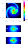 |
Fig. 14 Equatorial density distribution of the gas in the extended version of our best-fit model, which intends to include not only CO-rich gas, but also the adjacent regions in which molecules are assumed to be photodissociated (see Sect. 4.3 for details.) Top: density distribution in the plane of the equator. Middle: density distribution in the y = 0 plane. Bottom: same, but for the x = 0 plane. All representations share the same units and scales as in Fig. 6. |
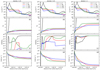 |
Fig. 15 Selected input and output quantities of the PDR models shown as a function of the distance from the white dwarf. We consider three models, shown from left to right, in which the density is one-third, half, and one times that of the extended heuristic model (see text), respectively. The different panels show from top to bottom (a) the density of H nuclei nH (note the peak reached at a distance of ~2 × 1014 cm for Λ = 0°, which stands for the position of the AGB star), (b) the visual extinction AV measured from the WD, (c), the fractional abundance of CO relative to H nuclei n(CO)/NH, and (d) the photodissociation rate of CO, Γ(CO). The verticaldotted line at the left edge is the position of the Strömgren radius. |
5 Conclusions
We have performed ALMA observations of R Aqr, a well-known SS. This system is composed of an AGB star plus a hot and compact WD, orbiting with a relatively long period of about 42 yr. The system is known to show strong interaction and spectacular symbiotic phenomena. The stars are surrounded by an extended nebula that is detected at several wavelengths, which shows an equatorial structure plus axial high-velocity jets, probably the result of accretion by the compact stellar component of material previously ejected by the AGB star. In Sect. 1 we discussed the properties of this system that are relevant for our study. Molecular lines are typically very weak in SSs; R Aqr is by far the symbiotic system that shows the richest and strongest molecular emission, although it presents very weak CO lines compared with standard AGB stars (Sect. 3).
We present high-quality maps of R Aqr in several CO lines, namely 12CO J = 2−1, J = 3−2, and J = 6−5 and 13CO J = 3−2 (Sects. 2 and 3). For 12CO J = 2−1 and J = 3−2, maps using different array configurations have been obtained, leading to higher and lower angular resolutions. The corresponding results have been compared, also taking single-dish data into account, and we deduce that most CO emission is detected in the interferometric maps, whichare a good representation of the actual CO-emitting region. The analysis of the maps of different lines indicates that the 12CO emission is partially opaque and comes from gas with a relative high excitation, typically with several hundred K.
The observations show a strongly structured and compact emitting region, occupying less than 1.″ 5. CO is emitted from a central intense clump, about 0.″ 2 wide, plus an elongated region formed by various arcs, which look like shreds of spiral arms. From a comparison with our knowledge on the binary system, we deduce that the relatively extended arcs are significantly focused on the equator of the system. Thebrightness distributions observed in R Aqr are highly different from those of standard AGB stars, in which observationssimilar to ours usually show arcs or incomplete spiral arms, but within an extended overall structure that is spherical or shows a moderate axial symmetry (Sect. 3).
Spiral structures in the nebula around SSs are predicted by hydrodynamical models of gravitational interaction between the wind of the primary and the compact companion. We have developed a heuristic, descriptive model of the CO-emission maps (Sect. 4.1) based on general results from hydrodynamical modeling. The model is 3D, and the geometry only assumes plane symmetry with respect to the equator. From the given distributions of the density, temperature, and velocity of the CO-rich gas, our code predicts velocity-channel maps that can be directly compared with the observations.
Our best-fit descriptive model, which is able to reproduce the observations quite satisfactorily, is composed of a central expanding condensation and several arcs showing both expansion and rotation movements. We identified a number of components (Sect. 4.1) in the CO-rich nebula: a central condensation (component A), a first arm associated with the WD (components B and C), and outer arms (components D and W, which are sometimes weak and patchy). There are also still weaker clumps (W′), as well as a component of uncertain origin (labeled ?) that could be due to infalling material. The central condensation occupies about 5 × 1014 cm, slightly more than the orbit, and the arcs occupy about 2 × 1015 cm in the equatorial plane, significantly less in altitude from the equator. The involved velocities range between 3 and 15 km s−1. The fastest rotation appears close to the WD. Our modeling confirms that only some threads of the spiral arms are detected, the remainder appears to show no significant CO emission.
As mentioned, this heuristic nebula model is compatible with our general ideas on hydrodynamical interaction in an SS. We also performed sophisticated calculations specifically for this case, see Sect. 4.2. This hydrodynamical modeling includes the gravitational attraction of both stars on the circumstellar material, as well as the hydrodynamical basic physics and radiative cooling, leading to nebular structures that depend on the orbital phase. Although our comparison of the two models can only be semiquantitative, the agreement between the hydrodynamical predictions and our heuristic/descriptive model of the CO line emission is very satisfactory, provided that we also take into account the high degree of CO photodissociation expected in some regions (see below). All the different components of our heuristic modeling can also be identified in the hydrodynamical simulations (Sect. 4.2, Fig. 10). We underline that our simulations assuming a relatively high eccentricity show prominent C and D components, notably with a density cavity in between, in agreement with the well-defined observed features, a property that does not appear in calculations assuming a circular orbit. The model also predicts infall in certain regions.
Even with the caveat that photodissociation significantly affects the distribution of CO molecules, several discrepancies subsist. The central condensation shows a very complex dynamics in the hydrodynamical modeling that is dominated by rotation and also shows expansion and infall. We did not try to incorporate this intricacy into our simple heuristic modeling (but assumed an isolated-AGB-like kinematics in the central region); in addition, the predicted rotation would yield a variation in velocity along the east–west direction that is not observed. The structure and dynamics of the spiral arms are remarkably well compatible with the hydrodynamical calculations, including the rotation and expansion velocity fields, except that the velocity moduli tend to be slightly higher in the descriptive models (i.e., in the observations).
Hydrodynamical models in general yield nebulae that are significantly more extended than observed in R Aqr. These predictions also show density contrasts that are in general much lower than those suggested by our ALMA maps and their 3D description. We interpret these differences as due to photodissociation by the UV radiation from the hot WD, which is compatible with the lack of molecular emission in SSs (Sect. 4.3). We have performed a detailed analysis of the chemistry of the nebula around R Aqr. We discussed photodissociation by UV from the WD and selfshielding effects, CO reformation within a very complete chemical reaction network, and time-dependent phenomena due to the orbital movement. In general, we found that when the UV radiation is not strongly shielded, photodissociation is very fast and CO is destroyed. CO formation, which mainly depends on the density, is often slower. We conclude forR Aqr that this object shows a set of relevant parameters such that nebular CO is not photodissociated in some areas, but completely disappears in others, namely in regions with lower densities and that are more directly exposed to the WD radiation. (Chemical calculations tend to require slightly lower densities than those found from our heuristic model, but they are still compatible within the uncertainties.) In general, we expect a significantlack of CO in the interarms, regions far from the equator, and in equatorial regions at distances ≳ 2 × 1015 cm. Because all these regions are cyclically exposed to the UV following the orbital periods, the time dependence of the chemistry also helps to explain the lack of CO, particularly in the outer regions. These results from our chemical modeling are compatible with our description of the maps of R Aqr, at least qualitatively. They also explain the lack of molecular emission in other SSs, most of which show shorter orbital periods and thinner nebulae.
Acknowledgements
We are grateful to the anonymous referee for his/her thorough reading of the paper and to Dr. S. Mohamed for enlightening discussions during the first phases of this project. This work has been supported by the Spanish MICINN, grants AYA2016-78994-P, AYA2016-75066-C2-1-P, PID2019-105203GB-C2, PID2019-106110GB-I00, and PID2019-107115GB-C21, and by the National Science Centre, Poland, grant OPUS 2017/27/B/ST9/01940. M.A. acknowledges funding support from the Ramón y Cajal programme of Spanish MICIU (grant RyC-2014-16277) and from the European Research Council (ERC Grant 610256: NANOCOSMOS). H.K. acknowledges support by the National Research Foundation of Korea (NRF), grant funded by the Korea government (MIST) (No. 2021R1A2C1008928). This paper makes use of the following ALMA data: ADS/JAO.ALMA#2017.1.00363.S and 2018.1.00638.S. ALMA is a partnership of ESO (representing its member more states), NSF (USA) and NINS (Japan), together with NRC (Canada), MOST and ASIAA (Taiwan), and KASI (Republic of Korea), in cooperation with the Republic of Chile. The Joint ALMA Observatory is operated by ESO, AUI/NRAO and NAOJ.
Appendix A Limits of our LTE treatment of the CO excitation
In this appendix, we estimate the error we can make by assuming that the CO levels are in thermal equilibrium at the local temperature. We performed calculations of the populations by solving the statistical equilibrium equations under the assumption of very low optical depths. We showed that the CO rotational lines are mostly optically thin. The advantage of using this approximation is that the level populations do not depend on the various approximations we can follow to perform the calculations (LVG-like local approximations or nonlocal treatments for different gas distributions). The calculations were performed for the relevant physical conditions, that is, for typical values of the density and temperature in relevant regions of the model nebula, because other properties of the nebula have no effect under the optically thin approximation. We discuss the effects of this and other implicit assumptions below, but the comparison is very conclusive in any case.
In Fig. A.1, we show the ratios, RT, of the relative level populations calculated by solving the statistical equilibrium equations and the thermalized populations. We show the population ratios for the J = 2 and J = 6 levels; intermediate levels (like J = 3) show intermediate behaviors. The variations in intensities of the lines that leave or arrive at these levels must be of the same order as the variations in the level populations. The typical conditions of the main components considered in our modeling are represented in the figure. The deviation from thermalized populations is always negligible, smaller than 10% and very similar for the different levels, which results in negligible effects in the synthetic maps. Departures always tend to yield higher populations and therefore (slightly) higher intensities. The reason is that for the relatively high involved temperatures, far higher than the relevant level energies, the effect of underthermalization is that levels with very high J-numbers are less densely populated than in thermal equilibrium; the excitation temperatures of low-J levels are much less affected because the relevant transitions, such as those we observe, have much smaller A-coefficients. The result is that molecules must crowd together in these lower levels and the transitions joining them are (in our case, slightly) more intense that in the thermalized case.
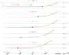 |
Fig. A.1 Ratios of the relative level populations calculated accurately by solving the statistical equilibrium equations for CO, assuming very low optical depths, and those calculated assuming thermalized level populations, RT. See the discussion in the text. We calculated RT for the J = 2 and J = 6 levels and for the conditions expected in our main model features A, B, C, D, and W, as indicated in the figure. The deviations from thermal equilibrium populations are in all cases <10%. |
These estimates are simple, but our approximations are not expected to affect our conclusions. We list the expected effects below:
To simplify our discussion in this appendix, we performed statistical equilibrium calculations assuming optically thin lines. Some opacity might be present, particularly if the nebulae shows clumpiness at a very small scale. However, opacity always tends to increase the thermalization degree (except for a few pathological cases, certainly not that of the single-ladder level structure of CO). Accounting for a certain degree of opacity will therefore lead to still more thermalized level populations and values of RT still closer to 1. We performed LVG calculations for optically thick cases and the other physical conditions adopted here, and this result was always confirmed: our calculations for low optical depths represent upper limits to the actual departures from thermalized populations.
We have claimed that CO is underabundant in less dense regions (e.g., far from the equator), and for this reason, they are not detected. The values of RT clearly tend to increase for lower densities. However, this effect would lead to relatively more intense emissions from these regions, which would lead to a still stronger discrepancy between predictions and observations. An “exact” treatment of the excitation in low-density regions will therefore reinforce our conclusion that CO is strongly underabundant in them.
Other uncertainties might be present, for instance, in the collisional transition coefficients. However, our results mostly depend on the level-integrated inelastic collisions, which have been well known for many years. Moreover, the departures form thermal equilibrium are very small in our case, and the effects of the uncertainties on collisional cross sections are very small, far smaller than the various sources of uncertainty in our general discussion. This result is also widely confirmed by various calculations: to increase RT by more that 1%, we must change the cross sections by more than 25%.
References
- Agúndez, M.,& Wakelam, V. 2013, Chem. Rev., 113, 8710 [CrossRef] [PubMed] [Google Scholar]
- Agúndez, M., Cernicharo, J., & Goicoechea, J. R. 2008, A&A, 483, 831 [NASA ADS] [CrossRef] [EDP Sciences] [Google Scholar]
- Agúndez, M., Cernicharo, J., Quintana-Lacaci, G., et al. 2017, A&A, 601, A4 [NASA ADS] [CrossRef] [EDP Sciences] [Google Scholar]
- Agúndez, M., Roueff, E., Le Petit, F., & Le Bourlot, J. 2018, A&A, 616, A19 [NASA ADS] [CrossRef] [EDP Sciences] [Google Scholar]
- Brugel, E. W., Cardelli, J. A., Szkody, P., et al. 1984, PASP, 96, 78 [CrossRef] [Google Scholar]
- Bujarrabal, V., Mikołajewska, J., Alcolea, J., & Quintana-Lacaci, G. 2010, A&A, 516, A19 [NASA ADS] [CrossRef] [EDP Sciences] [Google Scholar]
- Bujarrabal, V., Castro-Carrizo, A., Alcolea, J., et al. 2016, A&A, 593, A92 [NASA ADS] [CrossRef] [EDP Sciences] [Google Scholar]
- Bujarrabal, V., Alcolea, J., Mikołajewska, J., et al. 2018, A&A, 616, L3 [NASA ADS] [CrossRef] [EDP Sciences] [Google Scholar]
- Burgarella, D., Vogel, M., & Paresce, F. 1992, A&A, 262, 83 [Google Scholar]
- Castro-Carrizo, A., Quintana-Lacaci, G., Neri, R., et al. 2010, A&A, 523, A59 [NASA ADS] [CrossRef] [EDP Sciences] [Google Scholar]
- Cernicharo, J., Marcelino, N., Agúndez, M., et al. 2015, A&A, 575, A91 [NASA ADS] [CrossRef] [EDP Sciences] [Google Scholar]
- de Val-Borro, M., Karovska, M., Sasselov, D. D., & Stone, J. M. 2017, MNRAS, 468, 3408 [Google Scholar]
- Decin, L., Montargès, M., Richards, A. M. S., et al. 2020, Science, 369, 1497 [CrossRef] [Google Scholar]
- Fryxell, B., Olson, K., Ricker, P., et al. 2000, ApJS, 131, 273 [NASA ADS] [CrossRef] [Google Scholar]
- Gałan, C., Mikołajewska, J., Hinkle, K. H., et al. 2017, MNRAS, 466, 2194 [NASA ADS] [CrossRef] [Google Scholar]
- Gromadzki, M., & Mikołajewska, J. 2009, A&A, 495, 931 [NASA ADS] [CrossRef] [EDP Sciences] [Google Scholar]
- Gromadzki, M., Mikołajewska, J., Whitelock, P., et al. 2009, Acta Astron., 59, 169 [Google Scholar]
- Guélin, M., Patel, N. A., Bremer, M., et al. 2018, A&A, 610, A4 [NASA ADS] [CrossRef] [EDP Sciences] [Google Scholar]
- Homan, W., Danilovich, T., Decin, L., et al. 2018, A&A, 614, A113 [NASA ADS] [CrossRef] [EDP Sciences] [Google Scholar]
- Kaler, J. B. 1981, ApJ, 245, 568 [NASA ADS] [CrossRef] [Google Scholar]
- Kim, H., Hsieh, I.-T., Liu, S.-Y., et al. 2013, ApJ, 776, 86 [NASA ADS] [CrossRef] [Google Scholar]
- Kim, H., Trejo, A., Liu, S.-Y., et al. 2017, Nat. Astron., 1, 0060 [NASA ADS] [CrossRef] [Google Scholar]
- Kim, H., Liu, S.-Y., & Taam, R. E. 2019, ApJS, 243, 35 [NASA ADS] [CrossRef] [Google Scholar]
- Le Petit, F., Nehmé, C., Le Bourlot, J., & Roueff, E. 2006, ApJS, 164, 506 [NASA ADS] [CrossRef] [EDP Sciences] [Google Scholar]
- Mamon, G. A., Glassgold, A. E., & Omont, A. 1987, ApJ, 323, 306 [NASA ADS] [CrossRef] [Google Scholar]
- Meier, S. R., & Kafatos, M. 1995, ApJ, 451, 359 [NASA ADS] [CrossRef] [Google Scholar]
- Mikołajewska, J. 2012, Balt. Astron., 21, 5 [NASA ADS] [Google Scholar]
- Mikolajewska, J., Brandi, E., Hack, W., et al. 1999, MNRAS, 305, 190 [NASA ADS] [CrossRef] [Google Scholar]
- Min, C., Matsumoto, N., Kim, M. K., et al. 2014, PASJ, 66, 38 [NASA ADS] [CrossRef] [Google Scholar]
- Melnikov, S., Stute, M., & Eislöffel, J. 2018, A&A, 612, A77 [NASA ADS] [CrossRef] [EDP Sciences] [Google Scholar]
- Mohamed, S., & Podsiadlowski, P. 2012, Balt. Astron., 21, 88 [Google Scholar]
- Ramstedt, S., Mohamed, S., Olander, T., et al. 2018, A&A, 616, A61 [NASA ADS] [CrossRef] [EDP Sciences] [Google Scholar]
- Randall, S. K., Trejo, A., Humphreys, E. M. L., et al. 2020, A&A, 636, A123 [CrossRef] [EDP Sciences] [Google Scholar]
- Saberi, M., Vlemmings, W., Millar, T., & De Beck, E. 2019, in Why Galaxies Care About AGB Stars: A Continuing Challenge through Cosmic Time, IAU Symp., 343, 191 [Google Scholar]
- Saladino, M. I., Pols, O. R., van der Helm, E., et al. 2018, A&A, 618, A50 [NASA ADS] [CrossRef] [EDP Sciences] [Google Scholar]
- Schmid, H. M., Bazzon, A., Milli, J., et al. 2017, A&A, 602, A53 [NASA ADS] [CrossRef] [EDP Sciences] [Google Scholar]
- Smith, V. V., & Lambert, D. L. 1986, ApJ, 311, 843 [NASA ADS] [CrossRef] [Google Scholar]
- Solf, J., & Ulrich, H. 1985, A&A, 148, 274 [NASA ADS] [Google Scholar]
- Tielens, A. G. G. M., & Hollenbach, D. 1985, ApJ, 291, 722 [Google Scholar]
- Verbena, J. L., Bujarrabal, V., Alcolea, J., et al. 2019, A&A, 624, A107 [EDP Sciences] [Google Scholar]
- Wallerstein, G., & Greenstein, J. L. 1980, PASP, 92, 275 [NASA ADS] [CrossRef] [Google Scholar]
All Figures
|
Fig. 1 ALMA maps per velocity channel of 12CO J = 3−2 emission in R Aqr;see the LSR velocities in the upper left corners. The center is the centroid of the continuum, whose image has been subtracted. The contours are logarithmic, with a jump of a factor 2 and a first level of ±5 mJy beam−1, equal to 6.2times the rms and equivalent to 34.8 K (in Rayleigh–Jeans-equivalent brightness temperature units). The dashed contours represent negative values. The HPBW is shown in the inset in the last panel. |
| In the text | |
|
Fig. 2 ALMA maps per velocity channel of 12CO J = 3−2 emission in R Aqr obtained with a more compact ALMA configuration; see the LSR velocities in the upper left corners. The center is the centroid of the continuum, whose image has been subtracted. The contours are logarithmic, with a large jump of a factor 2 and a first level of ± 5 mJy beam−1 (equal to 3.4 times the rms and equivalent to 2.06 K). The dashed contours represent negative values. The HPBW is shown in the inset in the last panel. The represented field is wider than in our other maps. |
| In the text | |
|
Fig. 3 ALMA maps per velocity channel of 13CO J = 3−2 emission in R Aqr (only the more extended array configuration); see the LSR velocities in the upper left corners. The center is the centroid of the continuum, whose image has been subtracted. The logarithmic contours and scales are the same as in Fig. 1 (in this case, the first contour, 5 mJy beam−1, is equivalentto 5.6 times the rms and 35.2 K). The HPBW is shown in the inset in the last panel. |
| In the text | |
|
Fig. 4 ALMA maps per velocity channel of 12CO J = 2−1 emission in R Aqr; see the LSR velocities in the upper left corners, similar to Fig. 1. The contours are logarithmic, with a jump of a factor 2 and a first level of 4 mJy beam−1, equivalent to 4.9 rms and 11.33 K. The dashed contours represent negative values. The HPBW is shown in the inset in the last panel. |
| In the text | |
|
Fig. 5 ALMA maps per velocity channel of 12CO J = 6−5 emission in R Aqr; seethe LSR velocities in the upper left corners. The contours are logarithmic, with a jump of a factor 2 and a first level of 50 mJy beam−1, equivalent to 3.6 times the rms and 41.5 K. The dashed contours represent negative values. The HPBW is shown in the inset in the last panel. The velocity channels are the same as in Fig. 1, but the represented field is larger. The image center is the centroid of the continuum, whose image has not been subtracted (Sect. 2). |
| In the text | |
|
Fig. 6 Top: density distribution of the CO-rich gas in the plane of the equator (z = 0 plane in our coordinates) from our best-fit model. Equatorial velocities are also represented. Middle: density distribution in the y = 0 plane and velocities projected in that plane. Bottom: same, but for the x = 0 plane. All representations share the same units and scales. |
| In the text | |
|
Fig. 7 Predictions of our best-fit heuristic model for the 12CO J = 3−2 line maps, to be compared with observations, Fig. 1. All units and scales are the same as in Fig. 1. |
| In the text | |
|
Fig. 8 Top: main components identified in our simple model (see Sect. 4.1). Bottom (below the dotted line): Representative image of the equatorial density distribution as seen with the actual inclination of the equator. This image is a very simplified representation to facilitate interpretation, in which the latitude density distribution is not accounted for. The projection of the equatorial velocity in the direction to the observer is also represented (directly taken from the velocity vectors in Fig. 6, top). Again this is only illustrative because the off-equator movements are not considered. Downward arrows represent gas approaching the observer (relatively negative LSR velocities), while arrows pointing upward mean that the gas recedes from us (relatively positive LSR velocities). |
| In the text | |
|
Fig. 9 Representation of the different observed features (from Fig. 1) and the components of our model (A, B, C, D, W, and ? in Fig. 8) that are responsible for the corresponding predicted emission. |
| In the text | |
|
Fig. 10 Top: hydrodynamical model versus (bottom) our heuristic model for (a, d) number density, (b, e) radial velocity, and (c, f) rotational velocity distributions of the gas in the equatorial plane. Color bars label in units of cm−3 for number density and km s−1 for velocities.The overlaid arrows represent the gas velocity vectors. The pericenter of WD is located on the straight white line, and the current orbital phase of the binary stars is at 65° before the pericenter. |
| In the text | |
|
Fig. 11 Density distribution of the gas in the hydrodynamical model in the (a) y = 0 and (b) x = 0 planes, revealing the vertical flattening onto the equatorial plane. The velocity vectors show the fallback of gas toward the equatorial plane and the AGB star from up to the height of 50 AU. |
| In the text | |
|
Fig. 12 Top: column-density channel maps of our hydrodynamical model at an inclination of 15° from the edge-on view of the equatorial plane, and (bottom) the same, but with a pseudo-restriction of the density distributionup to a height of 15 AU. The central velocity of each channel with respect to the systemic velocity (~ − 24.5 km s−1 LSR) is indicated at the top left corner of each panel, and the individual channel width is 4 km s−1. Color bars are in units of g cm−2 (km s−1)−1. |
| In the text | |
|
Fig. 13 Position-velocity diagram of our hydrodynamical model at an inclination of 15° from the edge-on view of the equator. The velocity is measured with respect to the systemic velocity. The color bar is in units of g cm−2 (km s−1)−1. See observations in Bujarrabal et al. (2018). |
| In the text | |
|
Fig. 14 Equatorial density distribution of the gas in the extended version of our best-fit model, which intends to include not only CO-rich gas, but also the adjacent regions in which molecules are assumed to be photodissociated (see Sect. 4.3 for details.) Top: density distribution in the plane of the equator. Middle: density distribution in the y = 0 plane. Bottom: same, but for the x = 0 plane. All representations share the same units and scales as in Fig. 6. |
| In the text | |
|
Fig. 15 Selected input and output quantities of the PDR models shown as a function of the distance from the white dwarf. We consider three models, shown from left to right, in which the density is one-third, half, and one times that of the extended heuristic model (see text), respectively. The different panels show from top to bottom (a) the density of H nuclei nH (note the peak reached at a distance of ~2 × 1014 cm for Λ = 0°, which stands for the position of the AGB star), (b) the visual extinction AV measured from the WD, (c), the fractional abundance of CO relative to H nuclei n(CO)/NH, and (d) the photodissociation rate of CO, Γ(CO). The verticaldotted line at the left edge is the position of the Strömgren radius. |
| In the text | |
|
Fig. A.1 Ratios of the relative level populations calculated accurately by solving the statistical equilibrium equations for CO, assuming very low optical depths, and those calculated assuming thermalized level populations, RT. See the discussion in the text. We calculated RT for the J = 2 and J = 6 levels and for the conditions expected in our main model features A, B, C, D, and W, as indicated in the figure. The deviations from thermal equilibrium populations are in all cases <10%. |
| In the text | |
Current usage metrics show cumulative count of Article Views (full-text article views including HTML views, PDF and ePub downloads, according to the available data) and Abstracts Views on Vision4Press platform.
Data correspond to usage on the plateform after 2015. The current usage metrics is available 48-96 hours after online publication and is updated daily on week days.
Initial download of the metrics may take a while.