| Issue |
A&A
Volume 651, July 2021
|
|
|---|---|---|
| Article Number | L12 | |
| Number of page(s) | 9 | |
| Section | Letters to the Editor | |
| DOI | https://doi.org/10.1051/0004-6361/202140913 | |
| Published online | 28 July 2021 | |
Letter to the Editor
A CHEOPS white dwarf transit search
1
Center for Space and Habitability, Gesellsschaftstrasse 6, 3012 Bern, Switzerland
e-mail: This email address is being protected from spambots. You need JavaScript enabled to view it.
2
Department of Astronomy, Stockholm University, AlbaNova University Center, 10691 Stockholm, Sweden
3
Department of Physics and Astronomy, University College London, London WC1E 6BT, UK
4
Observatoire de Genève, Université de Genève, Chemin des maillettes 51, 1290 Sauverny, Switzerland
Received:
29
March
2021
Accepted:
12
May
2021
Abstract
White dwarf spectroscopy shows that nearly half of white dwarf atmospheres contain metals that must have been accreted from planetary material that survived the red giant phases of stellar evolution. We can use metal pollution in white dwarf atmospheres as flags, signalling recent accretion, in order to prioritize an efficient sample of white dwarfs to search for transiting material. We present a search for planetesimals orbiting six nearby white dwarfs with the CHaracterising ExOPlanet Satellite (CHEOPS). The targets are relatively faint for CHEOPS, 11 mag < G < 12.8 mag. We used aperture photometry data products from the CHEOPS mission as well as custom point-spread function photometry to search for periodic variations in flux due to transiting planetesimals. We detect no significant variations in flux that cannot be attributed to spacecraft systematics, despite reaching a photometric precision of < 2 ppt in 60 s exposures on each target. We simulate observations to show that the small survey is sensitive primarily to Moon-sized transiting objects with periods between 3 h < P < 10 h, with radii of R ≳ 1000 km.
Key words: white dwarfs / instrumentation: photometers / techniques: photometric / planets and satellites: detection
© ESO 2021
1. Introduction
White dwarfs are the evolutionary end points of over 95% of all stars (Fontaine et al. 2001; Koester 2013). Given the ubiquity of small exoplanets orbiting Sun-like stars (Petigura et al. 2018), we seek to probe whether rocky planets survive stellar evolution and continue orbiting their host remnants into the white dwarf phase.
The existence of planetesimals and dust grains orbiting main sequence stars has been firmly established by the discovery and study of debris disks (for a review, see Wyatt 2008). Specifically, an infrared excess is detected relative to the stellar photosphere. The lifetimes of the dust grains associated with this infrared excess are typically orders of magnitude shorter than the disk lifetimes, implying the existence of (invisible) planetesimals that are constantly replenishing the dust population via collisions (Heng & Tremaine 2010). An alternative interpretation of the infrared excess is that they are due to a large population of failed planetesimals with a sufficient covering fraction to produce an observable infrared excess (Heng & Tremaine 2010). The study of debris disks motivates the study of observational signatures in white dwarfs that are of planetary origin.
There is clear spectroscopic evidence that rocky planetary material survives into the white dwarf phase (Zuckerman & Reid 1998; Zuckerman et al. 2003, 2007; Farihi et al. 2008, 2009, 2010a,b, 2012; Hermes et al. 2014; Rocchetto et al. 2015). Spectroscopy reveals that nearly half of all white dwarfs show absorption lines due to metal pollution in their atmospheres (Wilson et al. 2019). Since metals have a finite lifetime in white dwarf atmospheres before sinking out of view, the presence of metals indicates recent accretion. Careful consideration of the chemical abundances present in white dwarf spectra have revealed that the accreted material must have been rock- and sometimes water-rich (Jura et al. 2009; Gänsicke et al. 2012; Farihi et al. 2013). Thus it appears that planetary bodies could survive into the white dwarf phase, which may provide a second era of habitability (Agol 2011).
Infrared excesses at some white dwarfs reveal the presence of debris disks containing ∼1000 K dust orbiting within 1 R⊙, which is much smaller and warmer than their main-sequence counterparts (Farihi 2016). These disks are found exclusively around polluted white dwarfs, and their infrared spectra have strong features from silicate grains, providing compelling evidence that the photospheric metals have a planetary origin (von Hippel et al. 2007; Jura et al. 2007; Farihi et al. 2012). The disks are hypothesized to be the end result of tidal disruptions of asteroids that have been perturbed onto highly eccentric orbits (Jura 2003).
Photometry of WD 1145+017 revealed disintegrating, likely rocky bodies orbiting a metal-polluted white dwarf (Vanderburg et al. 2015). Apparent transits of several dust clouds with orbital periods between 4 and 5 h were observed by the Kepler space telescope. The transit depths measured as large as 40%, and varied from transit to transit (Izquierdo et al. 2018; Xu et al. 2018). This system demonstrates the great potential of metal-polluted white dwarf planetary systems: (1) the spectroscopic detection of the metal pollution enhances transit search efficiency by looking at only white dwarfs with recent accretion histories; (2) the geometrical advantage afforded by the small radii of white dwarfs produces deep transits from small objects; (3) the orbits where transiting material may be found have periods of only a few hours; and (4) each transit transmits unique information about the rapidly changing system, which appears to evolve from one orbit to the next. Since the 2015 discovery, several further detections of transiting material have been made including the discovery of 20 day-long eclipses with a period of 107 days in optical photometry of ZTF J013906.17+524536.89 (Vanderbosch et al. 2020), and the discovery of transits of WD 1856+534 with a period of 1.4 days, corresponding to a Jupiter-sized occultor (Vanderburg et al. 2020).
The CHEOPS mission is a 30 cm effective-aperture telescope in low-Earth orbit since 2019 (Deline et al. 2020; Futyan et al. 2020; Hoyer et al. 2020). The spacecraft design is specified in Benz et al. (2021), and its initial performance is characterized by Lendl et al. (2020). In the first call for CHEOPS Guest Observer programs, we were awarded 84 orbits to search for transiting debris orbiting white dwarfs. We present the set of observations in AO-1 Program 7, completed in February 2021.
In Sect. 2, we provide a brief theoretical motivation for searches for transiting material on short orbital periods. In Sect. 3, we share two parallel analyses of the CHEOPS photometry with the data products produced by the CHEOPS team, as well as a reduction by a custom point-spread function (PSF) photometry package. In Sect. 4, we summarize a small simulation to estimate the detection efficiency of our CHEOPS observations in terms of sensitivity to planetsimal orbital period and radius. We discuss the implications of our observations in Sect. 5 and conclude in Sect. 6.
2. Theoretical motivation
The tidal disruption radius rc for circular orbits is approximately
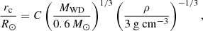 (1)
(1)
where C is a constant ranging from about 0.85 to 1.89 (see e.g.: Veras et al. 2014; Bear & Soker 2013). The period-density space of disrupted and intact bodies is shown in Fig. 1.
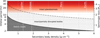 |
Fig. 1. Tidal disruption limits in period-density space for circular orbits (Veras et al. 2014). Vertical dashed lines mark the densities of several secondary bodies spanning a factor of five in bulk density from gas giant planets and rubble-pile asteroids through dense rocky bodies. Red regions of the plot represent regions where only single transit events may be detected in the CHEOPS photometry, nonred regions indicate where several occultations are possible within 24 h of photometry. The curves denote the regions where intact bodies may reside, the middle region marks potentially disrupted bodies, and black denotes bodies that we expect to be tidally disrupted. |
As we discuss later, we have observed the sample of white dwarfs in Table 1 for 24 h each, modulo the window function of Earth occultations. We required the minimum number of detected transits to be at least two in order to measure a periodic transiting event, so we only consider orbital periods ≲12 h. With these observations in mind as a guide, Fig. 1 suggests that rocky planetesimals with bulk densities similar to most small asteroids, ρ ≈ 1.9 g cm−3 (Fujiwara et al. 2006), should be tidally disrupted on orbital periods of P ≲ 4 h, may be tidally disrupted between 4 h < P < 12 h, and are likely intact otherwise.
CHEOPS white dwarf survey sample and the light curve precision in one minute exposures.
By surveying white dwarfs for objects with orbital periods of < 12 h, we are primarily sensitive to tidally disrupted material that has nearly circularized. This is consistent with the expectation that there is rocky material falling onto these white dwarfs based on the spectroscopic observations of metal pollution in their atmospheres.
3. Observations
The sample of metal-polluted white dwarfs observed with CHEOPS in AO-1 Program 7 is enumerated in Table 1. It includes six white dwarfs closer than 25 pc which span a factor of four in Teff.
In this work we consider the photometry produced with two methods, each processed with the same linear detrending as outlined in Sect. 3.1. In Sect. 3.2, we describe the standard aperture photometry products, and we revisit the same observations in Sect. 3.3 with PSF fitting photometry.
3.1. Linear detrending
The fluxes measured by the default aperture photometry from CHEOPS, f, contain several systematic trends as a function of the roll angle. To first order, the flux that we observe is a linear combination of the astrophysical signals we wish to detect and some unknown function of observational basis vectors. For some CHEOPS programs, the astrophysical signal has unconstrained quantities, such as transit times or depths. In principle, there is some design matrix X, which we can solve for the least-squares estimators  such that
 (2)
(2)
We provide a Python package to assemble a suitable design matrix from the CHEOPS data products called linea1, which by default concatenates a design matrix of a unit vector, and the cosine and sine of the roll angle, and we added the product of the sine and cosine of the roll angle as an additional basis vector. The roll angle terms account for the variations in flux that occur as a result of the rotation of the spacecraft.
3.2. CHEOPS data reduction pipeline (DRP) photometry
The DRP photometry contains corrections for dark and flat field normalization, bad pixels (pixels that are either hot or dead, and cosmic ray hits), and contamination from nearby stars in the aperture (Hoyer et al. 2020). After these corrections, the DRP measures the aperture photometry in four apertures of varying radii – we find that the DEFAULT aperture photometry produces a small median absolute deviation in the finished light curve, so we rely on that reduction for the DRP results presented here. The aperture radii for each target are listed in Table 1.
We masked outliers in the time series photometry by their corresponding stellar centroids by measuring the 4σ interval over which most stellar centroids reside, and by rejecting any fluxes for which the centroid exceeds this radius from the mean centroid position. On average, we rejected 4% of fluxes with this approach.
The DRP photometry reduced with the linear detrending described in Sect. 3.1 is shown in the left panels of Fig. A.1, and the corresponding box-least squares (BLS) periodograms are shown in the panels on the right. The DRP photometry has typical median absolute deviations similar to 1 ppt in 1 min exposures. Periodic signals are detected in the photometry that can usually be ascribed to aliases of the CHEOPS orbital period of 100 min (marked with vertical dashed lines in the periodograms). We observed that periodic single-point outliers tend to occur at the beginning and end of an orbit, which correspond to the times when the Earth is closest to the CHEOPS field of view, when stray light can be expected to be greatest (see Appendix C).
3.3. PSF photometry
To get an independent photometric extraction and potentially improve the precision, we adopted the PSF extraction tool PSF Imagette Photometric Extraction (PIPE) to use on the subarrays. Some advantages of using PSF photometry compared to aperture photometry are the following: (1) it can properly weigh the contribution to the signal of each pixel within the aperture to reduce the impact of the readout noise; (2) it is easier to filter out the impact of hot pixels and cosmic rays by identifying outlier pixels and removing them from the fit; and (3) the background can be fit simultaneously with the PSF to be less sensitive to spatial variations. A potential problem with this technique is that it can introduce noise due to a mismatch between the model and the actual PSF. CHEOPS was built to have a stable PSF, but in particular jitter (typically < 1 pix) will introduce motion blur during the 60 s exposures and modify the measured PSF. PIPE deals with motion blur by fitting a linear combination of model PSFs slightly offset from each other to the imagettes, improving the fit and leaving residuals dominated by photon noise. The model PSFs themselves were derived, one for each visit, by combining all observed frames within that visit.
The PIPE photometry, also reduced with the linear technique in Sect. 3.1, is shown in Fig. A.2. The PIPE photometry has typical median absolute deviations similar to 1 ppt in one-minute exposures, similar to the DRP photometry, but it performs better by up to a factor of two for the fainter targets. As with the DRP photometry, periodic signals are detected in the photometry which are usually aliases of the CHEOPS orbital period (marked with vertical dashed lines).
4. Transit simulations
We determined the probability of detecting a single transiting object with time series photometry by generating a series of 106 transit models, and by injecting them into the observations of our brightest and faintest targets using the open source Python package aspros2. We injected transits with the Mandel & Agol (2002) transit light curve model with orbital periods ranging from 3 h < P < 12 h, transiting object radii between 500 km < R < 2000 km, and assuming a fiducial white dwarf with RWD = 9 × 108 cm and MWD = 0.6M⊙.
We computed a BLS periodogram for each light curve, and measured the period with the strongest power and its aliases (Kovács et al. 2002). We measured the approximate signal-to-noise (S/N) of the candidate transit observations by measuring the significance of a transit model (fixed depth) compared with a transit-less model. If the S/N > 10, we considered the transit detected.
The period distribution of detected transiting objects is shown in Fig. 2. Typical detection efficiency is near 90% at orbital periods shorter than 5 hours, though it drops to 40–60% when the orbital period of the transiting object is an integer multiple of the CHEOPS orbital period, and as the period approaches 12 h.
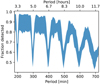 |
Fig. 2. Fraction of detected, simulated and injected transiting objects as a function of their orbital period. Aliases of the 100 min orbital period of CHEOPS are visible as drops in detection efficiency near integer multiples of 100 min. The upper limit of the shaded region represents the fraction of objects detected for the brightest white dwarf in the sample, and the lower limit marks the detection fraction for the faintest white dwarf. |
The radius distribution of detected objects is shown in Fig. 3. The BLS technique is most sensitive to objects roughly 1000 km in size or larger, which is about 60% of the lunar radius. Objects of this size can be thought of as monolithic planetesimals, rather than small rubble-piles asteroids (Lineweaver & Norman 2010).
 |
Fig. 3. Fraction of detected, simulated and injected transiting objects as a function of their radii. Objects with radii > 1000 km are more likely than not to be detected with S/N > 10 around any of the six white dwarfs. As in Fig. 2, the upper and lower limits of the shaded region mark the detected fraction of transiting objects for the brightest and faintest of the six white dwarfs. |
5. Discussion
5.1. DRP versus PIPE photometry
We have presented the results processed with the CHEOPS DRP and with the custom PSF photometry pipeline PIPE, see Figs. A.1 and A.2 and the median absolute deviations (MADs) in each light curve in Table 1. In most cases, the DRP and PIPE photometry have similar MADs, though PIPE photometry yields smaller scatter than DRP photometry for the faintest targets by nearly a factor of two. We recommend PSF photometry for deep searches for transits with CHEOPS on faint targets (V > 12 mag), and for brighter targets the DRP photometry should suffice.
5.2. Transit probability
The geometric transit probability for an Earth-sized planet orbiting a 0.6 M⊙ white dwarf in a 250 min orbit is 3%, implying that ∼30 stars must be surveyed in order to have an appreciable chance of finding a single transiting object, assuming all white dwarfs host transiting material. As in Agol (2011), if we wanted to measure the white dwarf planet occurrence rate η to a precision of 0.3 (e.g., nine planets discovered total), we would need to survey ∼300η−1 white dwarfs. Even in the optimistic scenario that η ≈ 1 for metal-polluted white dwarfs, we would require an observing program 50 times larger than the observations presented here to discover a new transiting planetesimal orbiting a white dwarf. For these reasons, we advocate here for continuing the transit search with wide-angle photometry from observatories such as TESS (Ricker et al. 2014), LSST (Lund et al. 2018), or Evryscope (Law et al. 2015), which combined will measure hundreds of light curves of white dwarfs. Narrow, deep campaigns such as the one presented here and in Wallach et al. (2018) for example, suggest that if transiting material were ubiquitous in orbit around white dwarfs, it would likely be quite small (Rp ≲ 1000 km) or orbiting at periods longer than about P ≳ 8 h.
5.3. Dust-free systems
By adapting the survival models of Heng & Tremaine (2010), Veras & Heng (2020) show that transit detections are possible in systems without significant dust disks by the delivery of intact planetesimals to close-in orbits at any cooling age. This reasoning suggests that transiting debris is perhaps likely orbiting white dwarfs regardless of metal pollution, so it may be fruitful to expand upon the work here to collect photometry of other bright, nearby white dwarfs that may host transiting debris without spectroscopic evidence of metal pollution.
6. Conclusion
We present the first search for transiting planetismals orbiting white dwarfs with the high precision photometry mission CHEOPS. The spacecraft can perform subpart-per-thousand photometry on targets as faint as G = 12.75 mag with minimal data processing steps by the user. We find that our small sample of six metal-polluted white dwarfs showed no significant transit-like events in the 24 h that each target was observed. The exceptional quality photometry would have been sensitive to transiting material ≳1000 km in radius on orbital periods ≲5 h, but no such material was detected.
Acknowledgments
We are grateful for helpful mission support from Kate Isaak, and for valuable feedback from Jay Farihi. CHEOPS is an ESA mission in partnership with Switzerland with important contributions to the payload and the ground segment from Austria, Belgium, France, Germany, Hungary, Italy, Portugal, Spain, Sweden, and the United Kingdom. This work has been carried out in the framework of the PlanetS National Centre of Competence in Research (NCCR) supported by the Swiss National Science Foundation (SNSF). This research has made use of the VizieR catalogue access tool, CDS, Strasbourg, France (DOI: 10.26093/cds/vizier). The original description of the VizieR service was published in A&AS 143, 23. AS acknowledges support from a Science and Technology Facilities Council studentship. We gratefully acknowledge the open source software which made this work possible: astropy (Astropy Collaboration 2013, 2018), ipython (Pérez & Granger 2007), numpy (Harris et al. 2020), scipy (Virtanen et al. 2020), matplotlib (Hunter 2007), synphot (STScI development Team 2018), batman (Kreidberg 2015), lightkurve (Lightkurve Collaboration 2020).
References
- Agol, E. 2011, ApJ, 731, L31 [NASA ADS] [CrossRef] [Google Scholar]
- Astropy Collaboration (Robitaille, T. P., et al.) 2013, A&A, 558, A33 [NASA ADS] [CrossRef] [EDP Sciences] [Google Scholar]
- Astropy Collaboration (Price-Whelan, A. M., et al.) 2018, AJ, 156, 123 [Google Scholar]
- Bear, E., & Soker, N. 2013, New Astron., 19, 56 [NASA ADS] [CrossRef] [Google Scholar]
- Benz, W., Broeg, C., Fortier, A., et al. 2021, Exp. Astron., 51, 109 [Google Scholar]
- Deline, A., Queloz, D., Chazelas, B., et al. 2020, A&A, 635, A22 [NASA ADS] [CrossRef] [EDP Sciences] [Google Scholar]
- Farihi, J. 2016, New Astron. Rev., 71, 9 [NASA ADS] [CrossRef] [Google Scholar]
- Farihi, J., Becklin, E. E., & Zuckerman, B. 2008, ApJ, 681, 1470 [NASA ADS] [CrossRef] [Google Scholar]
- Farihi, J., Jura, M., & Zuckerman, B. 2009, ApJ, 694, 805 [NASA ADS] [CrossRef] [Google Scholar]
- Farihi, J., Jura, M., Lee, J. E., & Zuckerman, B. 2010a, ApJ, 714, 1386 [NASA ADS] [CrossRef] [Google Scholar]
- Farihi, J., Barstow, M. A., Redfield, S., Dufour, P., & Hambly, N. C. 2010b, MNRAS, 404, 2123 [NASA ADS] [Google Scholar]
- Farihi, J., Gänsicke, B. T., Wyatt, M. C., et al. 2012, MNRAS, 424, 464 [NASA ADS] [CrossRef] [Google Scholar]
- Farihi, J., Gänsicke, B. T., & Koester, D. 2013, Science, 342, 218 [NASA ADS] [CrossRef] [Google Scholar]
- Fontaine, G., Brassard, P., & Bergeron, P. 2001, PASP, 113, 409 [NASA ADS] [CrossRef] [Google Scholar]
- Fujiwara, A., Kawaguchi, J., Yeomans, D. K., et al. 2006, Science, 312, 1330 [NASA ADS] [CrossRef] [PubMed] [Google Scholar]
- Futyan, D., Fortier, A., Beck, M., et al. 2020, A&A, 635, A23 [NASA ADS] [CrossRef] [EDP Sciences] [Google Scholar]
- Gänsicke, B. T., Koester, D., Farihi, J., et al. 2012, MNRAS, 424, 333 [NASA ADS] [CrossRef] [Google Scholar]
- Gentile Fusillo, N. P., Tremblay, P.-E., Gänsicke, B. T., et al. 2019, MNRAS, 482, 4570 [NASA ADS] [CrossRef] [Google Scholar]
- Harris, C. R., Millman, K. J., van der Walt, S. J., et al. 2020, Nature, 585, 357 [CrossRef] [PubMed] [Google Scholar]
- Heng, K., & Tremaine, S. 2010, MNRAS, 401, 867 [NASA ADS] [CrossRef] [Google Scholar]
- Hermes, J. J., Gänsicke, B. T., Koester, D., et al. 2014, MNRAS, 444, 1674 [NASA ADS] [CrossRef] [Google Scholar]
- Holberg, J. B., Bruhweiler, F. C., & Andersen, J. 1995, ApJ, 443, 753 [NASA ADS] [CrossRef] [Google Scholar]
- Hoyer, S., Guterman, P., Demangeon, O., et al. 2020, A&A, 635, A24 [NASA ADS] [CrossRef] [EDP Sciences] [Google Scholar]
- Hunter, J. D. 2007, Comput. Sci. Eng., 9, 90 [NASA ADS] [CrossRef] [Google Scholar]
- Izquierdo, P., RodrÃguez-Gil, P., Gänsicke, B. T., et al. 2018, MNRAS, 481, 703 [NASA ADS] [CrossRef] [Google Scholar]
- Jura, M. 2003, ApJ, 584, L91 [Google Scholar]
- Jura, M., Farihi, J., & Zuckerman, B. 2007, ApJ, 663, 1285 [NASA ADS] [CrossRef] [Google Scholar]
- Jura, M., Muno, M. P., Farihi, J., & Zuckerman, B. 2009, ApJ, 699, 1473 [NASA ADS] [CrossRef] [Google Scholar]
- Koester, D. 2013, in White Dwarf Stars, eds. T. D. Oswalt, & M. A. Barstow, 4, 559 [Google Scholar]
- Koester, D., Rollenhagen, K., Napiwotzki, R., et al. 2005, A&A, 432, 1025 [NASA ADS] [CrossRef] [EDP Sciences] [Google Scholar]
- Kovács, G., Zucker, S., & Mazeh, T. 2002, A&A, 391, 369 [NASA ADS] [CrossRef] [EDP Sciences] [Google Scholar]
- Kreidberg, L. 2015, PASP, 127, 1161 [NASA ADS] [CrossRef] [Google Scholar]
- Law, N. M., Fors, O., Ratzloff, J., et al. 2015, PASP, 127, 234 [NASA ADS] [CrossRef] [Google Scholar]
- Lendl, M., Csizmadia, S., Deline, A., et al. 2020, A&A, 643, A94 [EDP Sciences] [Google Scholar]
- Lightkurve Collaboration (Cardoso, J. V. D. M., et al.), Lightkurve: Kepler and TESS time series analysis in Python [Google Scholar]
- Lineweaver, C. H., & Norman, M. 2010, ArXiv e-prints [arXiv:1004.1091] [Google Scholar]
- Lund, M. B., Pepper, J. A., Shporer, A., & Stassun, K. G. 2018, AAS J., submitted [arXiv:1809.10900] [Google Scholar]
- Mandel, K., & Agol, E. 2002, ApJ, 580, L171 [NASA ADS] [CrossRef] [Google Scholar]
- McCleery, J., Tremblay, P.-E., Gentile Fusillo, N. P., et al. 2020, MNRAS, 499, 1890 [Google Scholar]
- Pérez, F., & Granger, B. E. 2007, Comput. Sci. Eng., 9, 21 [Google Scholar]
- Petigura, E. A., Marcy, G. W., Winn, J. N., et al. 2018, AJ, 155, 89 [NASA ADS] [CrossRef] [Google Scholar]
- Ricker, G. R., Winn, J. N., Vanderspek, R., et al. 2014, in Space Telescopes and Instrumentation 2014: Optical, Infrared, and Millimeter Wave, eds. J. Oschmann, M. Jacobus, M. Clampin, G. G. Fazio, & H. A. MacEwen, SPIE Conf. Ser., 9143, 914320 [Google Scholar]
- Rocchetto, M., Farihi, J., Gänsicke, B. T., & Bergfors, C. 2015, MNRAS, 449, 574 [Google Scholar]
- STScI development Team 2018, synphot: Synthetic photometry using Astropy, Astrophys. Source Code Libr. [record ascl:1811.001] [Google Scholar]
- van Maanen, A. 1917, PASP, 29, 258 [Google Scholar]
- Vanderbosch, Z., Hermes, J. J., Dennihy, E., et al. 2020, ApJ, 897, 171 [Google Scholar]
- Vanderburg, A., Johnson, J. A., Rappaport, S., et al. 2015, Nature, 526, 546 [NASA ADS] [CrossRef] [Google Scholar]
- Vanderburg, A., Rappaport, S. A., Xu, S., et al. 2020, Nature, 585, 363 [Google Scholar]
- Veras, D., & Heng, K. 2020, MNRAS, 496, 2292 [Google Scholar]
- Veras, D., Leinhardt, Z. M., Bonsor, A., & Gänsicke, B. T. 2014, MNRAS, 445, 2244 [Google Scholar]
- Virtanen, P., Gommers, R., Oliphant, T. E., et al. 2020, Nat. Meth., 17, 261 [Google Scholar]
- von Hippel, T., Kuchner, M. J., Kilic, M., Mullally, F., & Reach, W. T. 2007, ApJ, 662, 544 [Google Scholar]
- Wallach, A., Morris, B. M., Branton, D., et al. 2018, Res. Notes. Am. Astron. Soc., 2, 41 [Google Scholar]
- Wesemael, F., Henry, R. B. C., & Shipman, H. L. 1984, ApJ, 287, 868 [Google Scholar]
- Wilson, T. G., Farihi, J., Gänsicke, B. T., & Swan, A. 2019, MNRAS, 487, 133 [Google Scholar]
- Wyatt, M. C. 2008, ARA&A, 46, 339 [NASA ADS] [CrossRef] [Google Scholar]
- Xu, S., Rappaport, S., van Lieshout, R., et al. 2018, MNRAS, 474, 4795 [Google Scholar]
- Zuckerman, B., & Reid, I. N. 1998, ApJ, 505, L143 [Google Scholar]
- Zuckerman, B., Koester, D., Reid, I. N., & Hünsch, M. 2003, ApJ, 596, 477 [Google Scholar]
- Zuckerman, B., Koester, D., Melis, C., Hansen, B. M., & Jura, M. 2007, ApJ, 671, 872 [Google Scholar]
Appendix A: Photometry and periodograms
We present the photometry from the CHEOPS DRP and PIPE PSF photometry in Figs. A.1 and A.2.
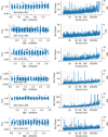 |
Fig. A.1. CHEOPS data reduction pipeline (DRP) light curves of six white dwarfs observed with the CHEOPS spacecraft in 2020 and 2021. Dashed vertical gray lines represent aliases of the CHEOPS orbital period (∼100 min). |
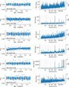 |
Fig. A.2. PIPE PSF photometry light curves of six white dwarfs observed with the CHEOPS spacecraft in 2020 and 2021. Compared with the DRP photometry in Fig. A.1, the PIPE photometry has a different sensitivity to detector artifacts and outliers. |
Appendix B: Validation of the CHEOPS photometry with TESS
Within about a year of each of the CHEOPS observations of these white dwarfs, the TESS spacecraft observed four out of the six white dwarfs studied in this work at two-minute cadence (Ricker et al. 2014). We performed a parallel analysis of these TESS observations to demonstrate that the CHEOPS non-detections presented above are in fact confirmed by the lack of photometric variability in the TESS observations.
We performed a similar BLS periodogram analysis to the one presented in Sect. 3 on the TESS observations and plot the results in Fig. B.1. No significant periodic events are detected with S/N > 5, indicating that indeed there is no transiting material orbiting these white dwarfs on periods of 10–300 min.
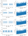 |
Fig. B.1. Same as Fig. A.1 presenting the two-minute cadence TESS observations of four of the six white dwarfs. No significant S/N > 5 periodic events are detected, confirming the lack of variability reported with CHEOPS. |
Appendix C: Masked fluxes
Figure C.1 shows the flux masking applied to the observations of WD 0046+051. The most severe flux outliers occur when the stellar centroid is most distant from the mean centroid position and also at the roll angle corresponding to the time immediately before Earth occultation near the roll angle of 50°, where the expected scattered light is greatest.
 |
Fig. C.1. Masking of outlier fluxes (red) compared with typical observations (black) based on the 4σ radius about the mean centroid. |
All Tables
CHEOPS white dwarf survey sample and the light curve precision in one minute exposures.
All Figures
|
Fig. 1. Tidal disruption limits in period-density space for circular orbits (Veras et al. 2014). Vertical dashed lines mark the densities of several secondary bodies spanning a factor of five in bulk density from gas giant planets and rubble-pile asteroids through dense rocky bodies. Red regions of the plot represent regions where only single transit events may be detected in the CHEOPS photometry, nonred regions indicate where several occultations are possible within 24 h of photometry. The curves denote the regions where intact bodies may reside, the middle region marks potentially disrupted bodies, and black denotes bodies that we expect to be tidally disrupted. |
| In the text | |
|
Fig. 2. Fraction of detected, simulated and injected transiting objects as a function of their orbital period. Aliases of the 100 min orbital period of CHEOPS are visible as drops in detection efficiency near integer multiples of 100 min. The upper limit of the shaded region represents the fraction of objects detected for the brightest white dwarf in the sample, and the lower limit marks the detection fraction for the faintest white dwarf. |
| In the text | |
|
Fig. 3. Fraction of detected, simulated and injected transiting objects as a function of their radii. Objects with radii > 1000 km are more likely than not to be detected with S/N > 10 around any of the six white dwarfs. As in Fig. 2, the upper and lower limits of the shaded region mark the detected fraction of transiting objects for the brightest and faintest of the six white dwarfs. |
| In the text | |
|
Fig. A.1. CHEOPS data reduction pipeline (DRP) light curves of six white dwarfs observed with the CHEOPS spacecraft in 2020 and 2021. Dashed vertical gray lines represent aliases of the CHEOPS orbital period (∼100 min). |
| In the text | |
|
Fig. A.2. PIPE PSF photometry light curves of six white dwarfs observed with the CHEOPS spacecraft in 2020 and 2021. Compared with the DRP photometry in Fig. A.1, the PIPE photometry has a different sensitivity to detector artifacts and outliers. |
| In the text | |
|
Fig. B.1. Same as Fig. A.1 presenting the two-minute cadence TESS observations of four of the six white dwarfs. No significant S/N > 5 periodic events are detected, confirming the lack of variability reported with CHEOPS. |
| In the text | |
|
Fig. C.1. Masking of outlier fluxes (red) compared with typical observations (black) based on the 4σ radius about the mean centroid. |
| In the text | |
Current usage metrics show cumulative count of Article Views (full-text article views including HTML views, PDF and ePub downloads, according to the available data) and Abstracts Views on Vision4Press platform.
Data correspond to usage on the plateform after 2015. The current usage metrics is available 48-96 hours after online publication and is updated daily on week days.
Initial download of the metrics may take a while.