| Issue |
A&A
Volume 651, July 2021
|
|
|---|---|---|
| Article Number | A22 | |
| Number of page(s) | 9 | |
| Section | Planets and planetary systems | |
| DOI | https://doi.org/10.1051/0004-6361/202140511 | |
| Published online | 05 July 2021 | |
Effect of solar wind density and velocity on the subsolar standoff distance of the Martian magnetic pileup boundary
1
State Key Laboratory of Lunar and Planetary Sciences, Macau University of Science and Technology,
Macau,
PR China
2
Institute of Space Weather, Nanjing University of Information Science and Technology,
Nanjing, PR China
3
CNSA Macau Center for Space Exploration and Science,
Macau,
PR China
4
State Key Laboratory of Space Weather, National Space Science Center, Chinese Academy of Sciences,
Beijing, PR China
e-mail: xielianghai@nssc.ac.cn
5
Joint Research and Development Center of Chinese Science Academy and Shen county,
Shandong,
PR China
6
Institute of Earth Sciences, Academia Sinica,
Taipei, Taiwan
e-mail: louclee@earth.sinica.edu.tw
7
Department of Physics and Space Science, Royal Military College of Canada,
Kingston,
ON, Canada
8
Planetary Environmental and Astrobiological Research Laboratory (PEARL), School of Atmospheric Sciences, Sun Yatsen University,
Zhuhai, PR China
Received:
8
February
2021
Accepted:
15
April
2021
Using a 3D multispecies magnetohydrodynamic model, we investigated the effect of the solar wind dynamic pressure (Pd) with different densities and velocities on the subsolar standoff distance (r0) of the Martian magnetic pileup boundary (MPB). We fixed the solar maximum condition, the strongest crustal field located in the dayside region, and the Parker spiral interplanetary magnetic field at Mars. We simulated 35 cases with a Pd range of 0.1494 to 7.323 nPa (solar wind number density n ∈ [1, 9] cm−3, and solar wind velocity V ∈ [−258, −1344] km s−1). The main results are as follows. (1) r0 decreases with increasing Pd according to the power-law relations. For the same Pd, a higher solar wind velocity (lower density) results in a larger r0 of the Martian MPB. (2) A higher solar wind density leads to a lower ratio of the compressed magnetic field strength to the crustal field strength and a larger plasma β under the same Pd. This indicates that the thermal pressure at the Martian MPB plays a significant role for the compressed magnetic field. Because the magnetic pileup process is stronger for a higher solar wind velocity, the magnetic pressure at the Martian MPB is increased. As a result, the thermal pressure decreases and r0 of the Martian MPB increases. (3) We present a new formula of r0 with the parameters of the solar wind dynamic pressure, number density, and velocity.
Key words: magnetohydrodynamics (MHD) / planets and satellites: terrestrial planets / planet-star interactions / solar wind
© ESO 2021
1 Introduction
The interaction of the solar wind with a terrestrial planet is one of the main topics in space physics. Typically, a magnetopause exits ahead of the planet with an intrinsic magnetic field, and the location of the planetary magnetopause is an important factor that reveals the nature of the interaction. Mars is a weakly magnetized planet with an atmosphere. The magnetic pileup boundary (MPB) or the induced magnetosphere boundary (IMB) at Mars can be created through mass loading and magnetic pileup processes. The MPB plays a similar role as the magnetopause (e.g., Edberg et al. 2009; Holmberg et al. 2019). The subsolar standoff point of the planetary magnetopause is the intersection of the line between the Sun and the planet and the planetary magnetopause; the subsolar standoff distance (r0) is measured from this point to the center of the planet (e.g., Shue et al. 1997; Edberg et al. 2008; Samsonov et al. 2020).
The r0 of Earth is controlled by the interaction of the terrestrial dipole magnetic field with the solar wind and has been studied for many years (e.g., Shue et al. 1997; Lin et al. 2010; Liu et al. 2015). In early theoretical studies, the magnetopause was assumed to be located at the place where the solar wind dynamic pressure (Pd) upstream of the bow shock balanced the magnetic pressure (PB) just inside the magnetopause (Chapman & Ferraro 1931). Here  , ρSW, and VSW are the mass density and velocity of the solar wind, respectively,
  , BM is the Earth’s magnetic field, and μ0 = 4π is the vacuum permeability. As a dipole magnetic field, BM is estimated approximately as BM = B0∕r3. Here B0 ≈ 31 100 nT
 represents the magnetic field strength on the equatorial surface of the Earth, which is associated with the dipole moment. As a result, a power-law relation was presented of the subsolar standoff distance r0 and Pd with the index − 1∕6 as follows (Beard 1960):
 (1)
(1)
This relation has been studied empirically, and most studies suggest an index smaller than − 1∕6 (Shue et al. 1997; Lin et al. 2010). In addition, other factors such as the interplanetary magnetic field (IMF) and the angle of the dipole tilt need to be taken into account (Lu et al. 2011; Liu et al. 2015). Recently, using global magnetohydrodynamic (MHD) simulations, Samsonov et al. (2020) found that r0 would be predicted more accurately by considering effects of ρSW and VSW individually, and suggested a new form of the relation,
 (2)
(2)
Moreover, Samsonov and collaborators also indicated that the changes in r0 for a velocity increase were greater than those for a density increase for the same Pd, especially for a southward IMF. In other words, the index M should be lower than N for the corresponding conditions. This also confirmed that owing to a higher solar wind velocity, the increased solar wind electric field would lead to a higher magnetopause reconnection rate and smaller r0 (e.g., Lee & Lee 2020).
Efforts have also been made to study the relation of r0 of the MPB (or IMB) and Pd for Mars, but the results are not yet as detailed as those for the Earth. Initially, because observations at Mars were scarce, only the averaged r0 was given for the common situation of Pd, such as 1.29 ± 0.04 RM (RM is the radius of Mars) in Vignes et al. (2000), 1.25 ± 0.03 RM in Trotignon et al. (2006), and 1.33 ± 0.15 RM in Edberg et al. (2008). As the number of observations increased, it was reported that the MPB boundary would move closer to the planet under the higher solar wind dynamic pressure conditions (e.g., Crider et al. 2003; Brain et al. 2005; Dubinin et al. 2007; Matsunaga et al. 2017). Specifically, using the observation of Phobos 2, Verigin et al. (1993) reported a power-law dependence of the asymptotic magnetotail diameter of the IMB on the solar wind dynamic pressure,  (the units of D and Pd are 103 km and dyn cm−2), where k ~ 5.9 ± 0.5, which was considered as the indicator of a global dipole magnetic field for Mars at the time. However, using data from Mars Global Surveyor (MGS) and Mars Express (MEX), Edberg et al. (2009) found an exponential dependence for the extrapolated terminator distance of the IMB on Pd, RT (RM) = 0.21(0.18Pd) + 1.34 (Pd is in nPa). Recently, also with MEX data, Ramstad et al. (2017) constructed a Martian IMB model with the parameters of the upstream solar wind density and velocity that showed that r0 of the IMB was located closer to the planet during a higher Pd. In contrast with Edberg et al. (2009), Ramstad et al. (2017) suggested that the Pd dependence on r0 should be presented by a power-law function and not by an exponential one. Specifically, the index of the power-law relation was approximately equal to − 1∕40 in their model, which was much larger than that for the Earth. In addition, Ramstad et al. (2017) also indicated that the IMB was mainly pressure-dependent, while changing ρSW or VSW individually had no significant effect for the equal dynamic pressure, which was inconsistent with the latest result of the Earth (Samsonov et al. 2020).
The pressure balance across a planetary magnetopause can affect its location, but the pressure effects on the Martian MPB are not yet fully understood. First, it is well accepted for the Earth that the magnetic pressure inside the magnetopause is approximately equal to the outside total pressure, which is mainly composed of the thermal and magnetic pressures at the subsolar region and converted by the upstream solar wind dynamic pressure (e.g., Wei et al. 2012; Shue & Chao 2013; Lu et al. 2015; Zhang et al. 2019). However, the pressure condition throughout the Martian MPB is more complex. It is generally accepted that dynamic, thermal, and magnetic pressure dominate in the region upstream of the bow shock, in the magnetosheath, and inside the MPB, respectively (e.g., Brain et al. 2010; Cui et al. 2018; Sánchez-Cano et al. 2020). It has been thought that the MPB was located at the place in which inside magnetic pressure and outside thermal pressure are balanced (Holmberg et al. 2019), but others indicated that the dynamic pressure was also important, especially in the flank regions (Xu et al. 2016; Matsunaga et al. 2017). For example, using multifluid MHD simulations, Xu et al. (2016) found that the boundary determined by the pressure ratio, β* = (Pth + Pd)∕PB = 1 (Pth, Pd, and PB are the thermal, dynamic, and magnetic pressure, respectively), agreed well with the ion composition boundary (ICB). In addition, Holmberg et al. (2019) regarded the magnetic pileup region as the region in which magnetic pressure dominated thermal pressure. They also indicated that the ionosphere and the magnetosheath could overlap the magnetic pileup region, which would result in complex pressure conditions near it. Very recently, Hardy et al. (2020) argued that for the Earth’s magnetosphere, which is relatively devoid of plasma inside the magnetopause boundary, the displacement of the Earth’s r0 was only determined by the outer Pd term. In contrast, for Saturn and Jupiter, the additional plasma β term (β is the ratio of the plasma thermal pressure to the magnetic pressure) could become more important because if β ≫ 1, an enhancement in internal plasma activity could act towards inflating the magnetosphere. In this way, a relative change in β had the same effect as a relative change in Pd. However, the pressure and β conditions at the Martian MPB have not yet been investigated in sufficient detail.
In this paper, using a three-dimensional multispecies MHD model, we study the effect and the mechanism of the solar wind dynamic pressure with different densities and velocities on the subsolar standoff distance of the Martian MPB. A new formula of r0 of the Martian MPB with the parameters of the solar wind dynamic pressure, number density, and velocity is presented.
2 Simulation and method
Similar to our previous study of the Martian bow shock (Wang et al. 2020a), the same three-dimensional multispecies MHD model that was originally developed by Ma et al. (2004) is employed to study the interaction of the solar wind and the Martian magnetosphere (Fang et al. 2010, 2015, 2017, 2018; Ma et al. 2014a,b).The input solar wind parameters in this model are the solar wind temperature (T), the solar wind number density (n), the components of the solar wind velocity (VX, VY, VZ), and the components of the interplanetary magnetic field (IMF) (BX, BY, BZ) in the Mars-centered solar orbital (MSO) coordinate system. The origin of this system is located at the Mars center, the X-axis points to the Sun, the Z-axis is normal to the Martian orbital plane, and the Y-axis completes the right-handed system. The numerical model of Ma et al. (2004) is implemented within the Space Weather Modeling Framework (SWMF; Tóth et al. 2012).
The computational domain of a typical simulation is defined as − 24 RM ≤ X ≤ 8 RM, − 16 RM ≤ Y, Z ≤ 16 RM, where RM = 3396 km is the radius of Mars, and the inner boundary is taken to be 100 km above the Martian surface. A nonuniform, spherical grid near Mars is applied for this model in which the radial resolution varies from 10 km at the lower boundary to 630 km at the outer boundary, while the resolution in longitude and latitude is uniform at 3°. The grid size is <0.01 RM in the radial direction within 1.20 RM ≤ r ≤ 1.40 RM, where the subsolar region of the Martian MPB is mainly located. The other details of the model are given in Ma et al. (2004).
In this model, the 60-order spherical harmonic model developed by Arkani-Hamed (2001) is applied to describe the crustal field and represents different orientations of Mars with respect to the solar wind direction. As the background Martian atmosphere or ionosphere condition is associated with the solar cycle condition or the solar extreme ultraviolet (EUV) radiation (e.g., Kim et al. 1998; Bougher et al. 2000; Lundin et al. 2013), the two fixed conditions of solar cycle maximum and minimum are adopted to describe the density profiles of the neutral species of the background Martian atmosphere, which are assumed to be spherically symmetric. We set these two model parameters in the same way as in Wang et al. (2020a) and Case 1 of Ma et al. (2004). Specifically, all the simulations were run under the solar maximum condition, and the subsolar location was fixed to 180° west longitude and 0° north latitude, which means that the strongest Martian crustal magnetic field is located in the dayside region (e.g., Crider et al. 2002; Fang et al. 2017). As a result, the season on Mars in the simulations was assumed to be the spring or autumn equinoxes. The crustal field orientations to the Sun are not the same at the solar longitude of Ls = 0 and Ls = 180.
In order to investigate the effect of the solar wind dynamic pressure with different densities and velocities on the subsolar standoff distance of the Martian MPB, we simulated 35 cases, as shown in Table 1. We worked with five sets of the solar wind number density, n = 1, 3, 5, 7, and 9 cm−3, five sets of solar wind velocities VX (while VY = VZ = 0) of −300, −400, −500, −600, and −700 km s−1, and two sets for Pd = 1 and 3 nPa. We obtain a Pd range of 0.1494 to 7.323 nPa.
It is also worth mentioning that the other input solar wind parameters for the cases in Table 1 are the same as Case 1 ofMa et al. (2004). That is, the upstream solar wind ion and electron temperatures were set to be 5 × 10⁴ and 3 × 10⁵ K, the solar wind velocities VY and VZ were chosen to be 0, and the IMF conditions were BX = − 1.6776 nT, BY = 2.4871 nT, and BZ = 0 nT, which represent the normal condition of the Parker spiral IMF (Parker 1958).
The first task was to determine the location of the MPB subsolar standoff point from the simulation data. As the Martian MPB is formed by mass loading and the magnetic pileup processes between the solar wind and the Martianatmosphere, some of the physical properties can be changed dramatically when the MPB is crossed from the magnetosheath to the Mars-induced magnetosphere. For example, sudden increases are expected in the magnitude of the magnetic field and the density of the predominantly planetary heavy ions (O+ and  ), combined with a corresponding decrease in the solar wind protons (H+) density, as well as a decrease in the fluctuations of the magnetic fields and the electron fluxes (e.g., Trotignon et al. 2006; Dubinin et al. 2007; Matsunaga et al. 2017). As a result, in previous observation studies, several corresponding methods were used to determine the location of the MPB, such as an increase in magnetic field strength and the absence of strong magnetic fluctuation (Matsunaga et al. 2015), the ratio of
  (Matsunaga et al. 2017), and the ratio of (Pth + Pd)∕PB (Xu et al. 2016). Similar determination methods were employed in numerical methods, such as the balance between the magnetic pressure and solar wind thermal pressure (Ma et al. 2014a). Moreover, Fang et al. (2015) obtained the 3D shape of the IMB by adopting the gradient of magnetic field magnitude to define the IMB location in the subsolar region (SZA < 15°) and the flowspeed gradient for the other region.
We worked with four methods to determine the possible locations of the MPB subsolar standoff point. Specifically, along the Sun-Mars line from the Sun to Mars, the subsolar standoff points are identified at the place where (1) the radially inward gradient of the plasma thermal pressure is minimized; (2) the radially inward gradient of the magnetic field magnitude reaches its second extreme maximum value; (3) the ratio of  ≥1.0; and (4) the ratio of (Pth + Pd)∕PB ≤ 1.0; as shown in Fig. 1. It is worth mentioning that the radially inward gradient of the magnetic field magnitude should be even greater in lower altitudes (generally <1.2 RM) because of the Martian intrinsic crustal field, and the bow shock is located at the place of the first extreme maximum value along the Sun-Mars line (Fang et al. 2015). Method (2) therefore chooses its second extreme maximum value along the Sun-Mars line to determine the subsolar standoff point of the Martian MPB.
Figure 1 shows the identified subsolar standoff distance (r0) for differentdetermination methods. Figure 1 shows that the identified r0 vary greatly in the different methods. The distances identified with the two methods of the gradient of the plasma thermal pressure and the gradient of the magnetic field magnitude are approximately the same for the same Pd, while the two methods of the ratio judgments yield similar results, especially for Pd ≥ 1 nPa. Generally, the values of the r0 identified bythe two gradient methods (the black circles and the red inverted triangles) are greater than those determined by the ratio methods (the blue squares and the green regular triangles), and the difference between them is about 0.1 RM.
We used the method of the gradient of the magnetic field magnitude to determine the subsolar standoff distance of the MPB for the following reasons. First, it is worth mentioning that we regard the MPB and IMB as the same boundary in which the magnetosheath magnetic fields are compressed and pile up, while the ICB is the boundary separating the solar wind plasma and the heavy ions in the induced magnetosphere (Wang et al. 2020b). In the theory of the MPB and IMB formation due to the mass loading process, the MPB and IMB and the ICB were located at the same locations, at least on the dayside (e.g., Breus et al. 1991; Matsunaga et al. 2017). However, several works have recently shown that the change in ion composition does not occur at thesame position as the changes in magnetic field strength and fluctuations, while the MPB and IMB are usually located farther from Mars than the ICB (e.g., Holmberg et al. 2019; Wang et al. 2020b). As a result, it is speculated that in this simulation work, the identified distances by the two gradient methods correspond to the r0 of the MPBand IMB, as described in the observations, and the ratio methods determine the r0 of the ICB. In this work, specifically, the r0 of the MPB is identified at the position where the radially inward gradient of the magnetic field magnitude reaches its second extreme maximum value along the Sun-Mars line.
Moreover, Fig. 1 also shows that r0 determined with the four methods decreases with increasing Pd, which agrees with the result of the previous work (e.g., Ramstad et al. 2017), and is discussed in detail next. For Pd < 1 nPa, it is somewhat unexpected that the distances determined by the ratio of (Pth + Pd)∕PB are larger than the distance determined by the ratio of  . In some cases, they are even greater than those by the two gradient methods. In other words, Fig. 1 shows that r0 of the pressure balance boundary would be greater than that of the ICB, and even greater than that of the MPB, for a low value of Pd < 1 nPa. This phenomenon partly agrees with the view of Holmberg et al. (2019) that the ionosphere and the magnetosheath might overlap the magnetic pileup region, and it is more obvious for a smaller Pd. The details of the phenomenon need to be verified and investigated in the future.
Pd sets of the simulation.
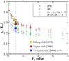 |
Fig. 1 Subsolar standoff distance (r0) identified with different determination methods. The black circles, red inverted triangles, blue squares, and green regular triangles stand for the distances identified by the method of the gradient of the plasma thermal pressure, the gradient of the magnetic field magnitude, the ratio of
|


3 Result and discussion
Next, we fit the dependence of Pd on r0 by the power-law and the exponential functions. The power-law function allows us to achieve a better fit than the exponential function, which also confirms the result of Ramstad et al. (2017). Therefore, we employed the power-law function to describe the relation of Pd and r0.
Figure 2 shows the solar wind dynamic pressure dependence on the subsolar standoff distance of the Martian MPB. The fitting result for the solid line (only considering Pd) is as follows:
 (3)
(3)
The determination coefficient of the fitting, R2, is the proportion of the variance in the dependent variable that can be predicted from the independent variable(s), and R2 = 1 corresponds to a perfect fitting. RMSE is the root mean squared error measured by the distance from the fitting result. The value of R2 is equal to 0.9710 and RMSE = 0.007931 for this fitting.
The fitting result when n and V are considered individually is as follows:
 (4)
(4)
Here, the units of n and V are cm−3 and km s−1. For this fitting result, R2 = 0.9907, RMSE = 0.004568.
Figure 2 and Eqs. (3) and (4) show that the dependence of r0 on Pd can be better presented by the power-law relations than by the exponential one, especially for the larger Pd (> 5 nPa). The values of R2 for the two power-law fittings are greater than 0.97, which implies a relatively high fitting goodness. The power-law index of Pd in this work (− 1∕25.84) is greater than that of the Earth (approximately −1∕6), which denotes a weaker intrinsic magnetic field and a relatively smaller variation of r0 for Mars. The power-law index in this work is lower than the − 1∕40 of Ramstad et al. (2017).
Figure 2 also shows that the differences in r0 for the different n and V but same Pd can reach ~0.05 RM. As the value of R2 = 0.9907 for two parameters fitting is higher than R2 = 0.9710 for a single Pd dependence (RMSE is correspondingly smaller), thePd dependence on r0 can be described more accurately by fitting n and V individually than by just fitting Pd. Moreover, our results show that for the same Pd, a higher solar wind density (and lower velocity) results in a smaller r0 of the Martian MPB.
Our results from the MHD simulation of the solar wind-Mars interaction agree with the work about the Earth’s magnetopause by Samsonov et al. (2020) that r0 would be predicted more accurately by taking the effects of ρSW and VSW individually into account rather than considering Pd alone. However, Samsonov et al. (2020) also indicated that the changes in r0 for a velocity change were greater than those for a density change for the same Pd, especially for a southward IMF, which implied that the power-law index of VSW, M, was lower than that of ρSW, N. We found a different result, however: A higher solar wind number density (or a lower velocity) results in a smaller r0 of the Martian MPB for thesame Pd (M > N). Moreover, these two results are also inconsistent with the results of Ramstad et al. (2017), who reported that the Martian IMB was mainly pressure-dependent and that changing ρSW or VSW individually had no significant effect for the equal dynamic pressure.
The mechanism for the different effects of ρSW and VSW on r0 for the Earth can be explained by the solar wind electric field. It is generally greater for a higher solar wind velocity, which leads to the enhanced magnetopause reconnection rate and Region 1 current, especially for a southward IMF (e.g., Lee & Lee 2020; Samsonov et al. 2020). As a result, the greater changes in r0 occur for a velocity increase and not for a density increase for the same Pd. For Mars, which is a weakly magnetized planet, the different results of ρSW and VSW effects cannot be explained by the traditional concept of the solar wind electric field and the reconnection conditions at the Earth. On the other hand, the location of the magnetopause can also be affected and described by the pressure balance across it, as we mentioned above. To investigate the reason for the opposite effects of ρSW and VSW at Mars as compared to Earth, we next studied the pressure balance throughout the MPB in more detail. Following Schield (1969) and Suvorova et al. (2010), we introduced a factor k and f that describe the contributions of the different components, both thermal and magnetic, of pressure to the total pressure.
We define the factor k as the ratio of the total pressure just outside the Martian MPB to the upstream solar wind dynamic pressure as follows:  . Here
  ,
,  , and
, and  are the plasma thermal pressure, the magnetic pressure, and the solar wind dynamic pressure just outside the subsolar standoff point of the Martian MPB, respectively.
 is the solar wind dynamic pressure upstream of the bow shock. As the plasma thermal pressure and the magnetic pressure upstream of the bow shock are very low and can be neglected, the factor k can be used to describe how much the upstream solar wind dynamic pressure is converted into thermal and magnetic pressure just outside the MPB. The theoretical value of k in a gas-dynamic approximation assuming a normal shock is 0.881 (Schield 1969). In addition, k also varies with the upstream solar wind and downstream magnetopause conditions (e.g., Suvorova et al. 2010). For a higher value of k, a higher ratio of
  is converted into the outside of the magnetopause, which would result in a more compressed magnetosphere and a smaller r0 (e.g., Shue & Chao 2013; Lu et al. 2015). It is worth mentioning that although the Pd is insignificant near the subsolar region of the MPB, we also took it into account to improve the calculation accuracy. The factor k is shown in panel a of Fig. 3.
The factor f is the strength ratio of the compressed (or actual) magnetic field to the pure crustal magnetic field at the subsolar point of the MPB as follows: f = Bcompressed∕Bcrustal. Here, the crustal field model of Arkani-Hamed (2001) was used, as we mentioned above. The theoretical values of f are 2 for a dipole confinement by an infinite plane and 2.44 for the Chapman-Ferraro problem (Beard 1964). For a higher value of f, the magnetic pressure inside the magnetopause is higher because the strength of the magnetic field increases, which would result in a larger r0 (e.g., Shue & Chao 2013; Lu et al. 2015).
Panels a and b of Fig. 3 show the solar wind dynamic pressure dependence on factors k and f for the different solar wind number densities. Figure 3 shows that k decreases and f increases with increasing Pd. The average value of k at the Martian MPB is ~0.9 and is slightly greater than the 0.88 at the Earth. The average value of f reaches 3.5, which is also larger than the 2.44 for the typical condition of the Earth. For the same Pd constituted with different n (or V), the values of the factor k are almost same, while the values off are different. Specifically, the value of f for a smallern is greater than that for a larger n for the same Pd. A higher value of f indicates a larger r0, as we mentioned above, therefore we can conclude that r0 is larger for a smaller n for the same Pd. As a result, the different effects of n and V on r0 for the same Pd are probably caused by the different values of the factor f and not by the factor k.
However, the reason for the larger f corresponding to a lower solar wind number density n for the same Pd is not clear. Very recently, Hardy et al. (2020) argued that for the Earth’s magnetosphere, which is relatively devoid of plasma inside the magnetopause boundary, the displacement of the subsolar standoff distance of the magnetopause is only determined by the outer Pd term. This situation is different from that of Saturn and Jupiter, for example, where the additional plasma β term (β is the ratio of the plasma thermal pressure to the magnetic pressure) could become more important because if β ≫ 1, an enhancement in internal plasma activity causes the magnetosphere to inflate. In this way, a relative change in β has the same effect as a relative change in Pd. In this vein, we further investigated the plasma β at the subsolar standoff point of the Martian MPB, as shown in panel c of Fig. 3, as well as the pressure terms along the Sun-Mars line (Fig. 4).
Panel c of Fig. 3 shows the dependence of the plasma β at the subsolar standoff point on the solar wind dynamic pressure dependence for the solar wind number density of n = 1 (cyan), 3 (black), 5 (red), 7 (blue), and 9 (green) cm−3. Panel c of Fig. 3 shows that the plasma β at the subsolar standoff point of the Martian MPB is enhanced with increasing Pd. The values of β are greater than 1 for most cases of Pd > 0.3 nPa, which indicates that the plasma thermal pressure dominates at the subsolar standoff point of the Martian MPB and not the magnetic pressure. The values of β for a higher solar wind number density n are generally greater than those for a smaller n for the same Pd, although the results for n = 9 cm−3 do not agree very well. In addition, this relation can be described by the following fitting result: β = 0.01417n0.5117V0.7447 (the units of n and V are cm−3 and km s−1).
Figure 4 shows the pressure profiles along the Sun-Mars line on the dayside which is under the same solar wind condition as case 1 of Ma et al. (2004) for panel a, in which Pd = 1 nPa (n = 4 cm−3 and V = 400 km s−1). Panel a of Fig. 4 displays that upstream of the bow shock (>1.63 RM), the solar wind dynamic pressure Pd (SW) dominates. In the magnetosheath, the Pd(SW) is rapidly converted into the solar wind thermal pressure Pth(SW); the magnetic pressure PB in the magnetosheath also increases slightly. At the subsolar standoff point of the MPB, Pth (SW) is greater than PB, and Pd (SW) decreases to nearly zero. Inside the MPB, Pth(SW) continues to decrease and PB continues to increase, while the ionosphere thermal pressure Pth(ion) is also higher at lower altitudes.
Panel b of Fig. 4 displays similar pressure profiles along the Sun-Mars line as in panel a for the different solar wind number densities for the same Pd. For n = 9 cm−3 Pth (SW) is larger and PB is smaller at the MPB compared with n = 1 cm−3. In other words, a higher solar wind density results in a higher thermal pressure (and β) at the subsolar standoff point of the Martian MPB. Moreover, as the thermal pressure is relatively more important than the magnetic pressure outside the Martian MPB, the higher thermal pressure (and β) due to the higher solar wind density n results in a smaller r0 of the Martian MPB. In addition, panel b also shows that the location of the Martian bow shock (~ 1.65 RM) for smaller n is also closer to Mars than that for larger n, which mightbe due to the corresponding changes in the solar wind velocity.
Panels c and d reveal that for n = 9 cm−3, the solar wind number density along the X line is greater than that for n = 1 cm−3, while the situation for the solar wind electron temperature is the reverse. As a result, the Pth (SW) at the magnetosheath does not change much for thedifferent n, as seen in panel b. This indicates that the larger upstream n cannot simply account for the larger Pth(SW) at the MPB, which we describe next. Moreover, the results from Fig. 4 remain similar for the other Pd cases for different n. It is also worth mentioning that the solar wind electron temperature Te upstream of the bow shock for n = 1 cm−3 is slightly higher than that for n = 9 cm−3 in panel c. We speculate that the higher Te in the n = 1 cm−3 case might be caused by the numerical diffusion. The reason is that the n = 1 cm−3 case has a larger magnetosonic Mach number Mms, which corresponds to the sharper changes in thermal pressure and temperature when across the bow shock. Accordingly, the numerical diffusion is more significant due to the larger gradients, which finally results in the higher Te upstream of the bow shock. However, this difference in Te does not affect the positions of either BS or MPB, and we therefore did not pursue the reasons for it further.
Figure 4 shows that the pressure conditions across the subsolar standoff point of the Martian MPB are different from those of the Earth. At the Earth, outside the subsolar standoff point of the magnetopause, thermal and magnetic pressures dominate, which are converted by the upstream solar wind dynamic pressure Pd, and the ratio of these two pressures is affected by the upstream solar wind conditions (Shue & Chao 2013; Lu et al. 2015). Inside the magnetopause, the magnetic pressure provided by the Earth’s dipole magnetic field absolutely dominates, while the solar wind plasma thermal pressure is not significant at all (e.g., Shi et al. 2013; Hardy et al. 2020). Outside the subsolar standoff point of the MPB, the situation for Mars is similar to that of the Earth, while inside the MPB, the solar wind plasma thermal pressure still plays an important role, in contrast to the Earth. In addition, our simulation also shows that the solar wind plasma thermal pressure is not negligible even inside the pressure balance boundary.
The mechanism for the enhanced thermal pressure (and β) at the MartianMPB for a higher solar wind density can be described by the magnetic pileup process, which is related tothe solar wind velocity. As a lower solar wind density denotes a higher velocity for the same Pd, the solar wind convection electric field (Econ = BIMF × V) is larger for the same IMF condition. As a result, the mass loading effect due to the pickup process is stronger, which results in a stronger magnetic pileup region (e.g., Modolo et al. 2006; Vaisberg et al. 2017; Chang et al. 2020). In this vein, the magnetic pressure at the Martian MPB should be higher for a higher solar wind velocity (or lower density), which is also shown in panel b of Fig. 4. In addition, when the magnetic field strength increases (the magnetic pressure increases), the plasmas near the plasma depletion region are squeezed out along the pileup magnetic field, leading to a decrease in plasma β, plasma density, and ion temperature, especially for the hotter plasmas (e.g., Lee & Lee 2020; Wang et al. 2020b). As a result, the thermal pressure at the Martian MPB decreases when the magnetic pressure increases due to the stronger magnetic pileup process for the higher solar wind velocity. Moreover, thermal pressure and magnetic pressure dominate in the magnetosheath and the magnetosphere, respectively (Brain et al. 2010; Sánchez-Cano et al. 2020). Therefore, a higher solar wind velocity (a lower density) results in a larger r0 of the Martian MPB for thesame Pd. The different results and mechanisms of the solar wind density and velocity effects on the r0 of Earth and Mars are summarized in Table 2.
Although the solar wind velocity and the magnetic pressure dominate the location of the Martian MPB, the thermal pressure also plays a significant role at the Martian MPB boundary compared with the condition on Earth. As a result, the pressurebalance equation across the Martian MPB should correspondingly be improved by another version,  , which is also suggested by Eq. (5) of Hardy et al. (2020). Moreover, as β is also related to the solar wind number density n and velocity V, r0 of the Martian MPB can be expressed by
  , as shown in Fig. 5.
Figure 5 shows the fitting results as follows:
 (5)
(5)
The value of R2 is equal to 0.9952, which is greater than the values of Eqs. (3) and (4), and RMSE = 0.004341, which is also the smallest. Both indexes indicate a better fitting goodness for this function. Figure 5 shows that r0 of the Martian MPB decreases with the solar wind dynamic pressure Pd according to the power-law relations. For the same Pd, a higher solar wind velocity (a lower density) results in a larger r0 of the Martian MPB.
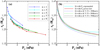 |
Fig. 2 Solar wind dynamic pressure dependence on the subsolar standoff distance of the Martian MPB. Panel a: r0 identified from the simulation data for the solar wind number density n = 1 (blue), 3 (cyan), 5 (black), 7 (green), and 9 (red) cm−3. The solid line segments connect adjacent points. Panel b: fitting results by the exponential function (solid cyan line), by the power-law relations considering Pd alone, |
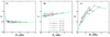 |
Fig. 3 Solar wind dynamic pressure dependence on the factor k (panel a), the factor f (panel b), and the plasma β (panel C) at the subsolar standoff point for the solar wind number density n = 1 (cyan), 3 (black), 5 (red), 7 (blue), and 9 (green) cm−3. |
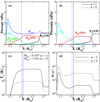 |
Fig. 4 Pressure profiles along the Sun-Mars line on the dayside with the same solar wind condition as in Case 1 of Ma et al. (2004) for panel a. The solid black, red, green, cyan, and blue lines represent the solar wind dynamic pressure Pd (SW), the solar wind plasma thermal pressure Pth(SW), the ionosphere thermal pressure Pth(ion), the magnetic pressure PB, and the totalpressure P(SW), respectively.The small circles indicate the positions of the radial grid points, and the vertical dashed line represents the identified location of the subsolar standoff point of the Martian MPB. Panel b: similar pressure profiles for n = 1 (solid lines) and 9 (dashed lines) cm−3 when Pd = 1 nPa. The black, red, and cyan lines stand for Pd(SW), Pth (SW), and PB, respectively. The vertical blue lines represent the corresponding identified locations of the subsolar standoff point of the Martian MPB. Panels c and d: corresponding conditions of the solar wind electron temperature (Te (K)) and thesolar wind number density (n (cm−3)) for panel b along the Sun-Mars line. |
Result and mechanism of the solar wind density and velocity effects on r0 of Earth and Mars.
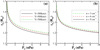 |
Fig. 5 Fitting results for |
4 Summary and conclusions
We used the 3D multispecies MHD model developed by Ma et al. (2004) to investigate the effect of the solar wind dynamic pressure with different densities and velocities on the subsolar standoff distance of the Martian MPB. We simulated 35 cases with values of Pd ranging from 0.1494 to 7.323 nPa (the solar wind number density n ∈ [1, 9] cm−3, the solar wind velocity V ∈ [−258, −1344] km s−1). After considering four different determination methods, we defined the subsolar standoff point of the Martian MPB at the position where the radially inward gradient of magnetic field magnitude reaches its second extreme maximum value along the Sun-Mars line. Our simulations show that the MPB is usually located farther from Mars than the ICB, which agrees with the latest observations of Holmberg et al. (2019) and Wang et al. (2020b), even in the subsolar region. The main results of this work are listed below.
- 1.
r0 of the Martian MPB decreases with increasing Pd according to the power-law relations. For the same Pd, a higher solar wind velocity (a lower density) results in a larger r0 of the Martian MPB.
- 2.
For the same Pd constituted with different solar wind densities and velocities, the values of factor
 are almost same, while the values of f = Bcompressed∕Bcrustal and plasma β are different. A higher solar wind density results in a smaller f and a larger plasma β for the same Pd, which indicates the significant role of the thermal pressure at the Martian MPB. Because the magnetic pileup process is stronger for the higher solar wind velocity, the magnetic pressure at the Martian MPB increases. As a result, the thermal pressure decreases and r0 of the Martian MPB becomes larger.
 - 3.
We also present a new formula of r0 of the Martian MPB with the parameters of the solar wind dynamic pressure, number density, and velocity.
The increasing observations of the Martian MPB crossings from the multiple satellites in the future will be used to further examine the relation of the location of the Martian MPB and the solar wind dynamic pressure with the different densities, as well as the pressure conditions across it. We fixed the crustal field located in the dayside region for all the cases, as well as the normal condition of the Parker spiral IMF at Mars. These factors may also affect the location of the Martian MPB and need to be further investigated in the future.
Acknowledgements
The work is supported by the National Natural Science Foundation of China (grant 42074195, 4030203, 41974190, 41974073, 41404053), the Science and Technology Development Fund (FDCT) of Macau (0035/2018/AFJ), and Macau Foundation and the pre-research project on Civil Aerospace Technologies No. D020104, D020308, and D020303 funded by China’s National Space Administration. The work is also supported by Beijing Municipal Science and Technology Commission (Grant No.Z191100004319001), a grant from the “Macao Young Scholars Program” (Project code: AM201905), and the opening fund of the State Key Laboratory of Lunar and Planetary Sciences (Macau University of Science and Technology; Macau FDCT grant No. 119/2017/A3). We acknowledge the CSEM team in University of Michigan for the use of BATS-R-US code. The numerical calculations in this paper have been carried out on the super computing system in the Super computing Center of Nanjing University of Information Science & Technology. We especially acknowledge Yingjuan Ma at UCLA for the multi-species MHD model used in this work.
References
- Arkani-Hamed, J. 2001, J. Geophys. Res., 106, 23197 [Google Scholar]
- Beard, D. B. 1960, J. Geophys. Res., 65, 3559 [Google Scholar]
- Beard, D. B. 1964, Rev. Geophys. Space Phys., 2, 335 [Google Scholar]
- Bougher, S. W., Engel, S., Roble, R. G., et al. 2000, J. Geophys. Res., 105, 17669 [Google Scholar]
- Brain, D. A., Halekas, J. S., Lillis, R., et al. 2005, Geophys. Res. Lett., 32, L18203 [Google Scholar]
- Brain, D., Barabash, S., Boesswetter, A., et al. 2010, Icarus, 206, 139 [Google Scholar]
- Breus, T. K., Krymskii, A. M., Lundin, R., et al. 1991, J. Geophys. Res., 96, 11165 [Google Scholar]
- Chang, Q., Xu, X., Xu, Q., et al. 2020, ApJ, 900, 63 [Google Scholar]
- Chapman, S., & Ferraro, V. C. A. 1931, J. Geophys. Res., 36, 77 [Google Scholar]
- Crider, D. H., Acuña, M. H., Connerney, J. E. P., et al. 2002, Geophys. Res. Lett., 29, 1170 [Google Scholar]
- Crider, D. H., Vignes, D., Krymskii, A. M., et al. 2003, J. Geophys. Res. Space Phys., 108, 1461 [Google Scholar]
- Cui, J., Yelle, R. V., Zhao, L.-L., et al. 2018, ApJ, 853, L33 [Google Scholar]
- Dubinin, E., Fränz, M., Woch, J., et al. 2007, The Mars Plasma Environment (Berlin: Springer), 209 [Google Scholar]
- Edberg, N. J. T., Lester, M., Cowley, S. W. H., et al. 2008, J. Geophys. Res. Space Phys., 113, A08206 [Google Scholar]
- Edberg, N. J. T., Brain, D. A., Lester, M., et al. 2009, Annal. Geophys., 27, 3537 [Google Scholar]
- Fang, X., Liemohn, M. W., Nagy, A. F., et al. 2010, J. Geophys. Res. Space Phys., 115, A04308 [Google Scholar]
- Fang, X., Ma, Y., Brain, D., et al. 2015, J. Geophys. Res. Space Phys., 120, 10, 926 [Google Scholar]
- Fang, X., Ma, Y., Masunaga, K., et al. 2017, J. Geophys. Res. Space Phys., 122, 4117 [Google Scholar]
- Fang, X., Ma, Y., Luhmann, J., et al. 2018, Geophys. Res. Lett., 45, 3356 [Google Scholar]
- Hardy, F., Achilleos, N., & Guio, P. 2020, Geophys. Res. Lett., 47, e86438 [Google Scholar]
- Holmberg, M. K. G., André, N., Garnier, P., et al. 2019, J. Geophys. Res. Space Phys., 124, 8564 [Google Scholar]
- Kim, J., Nagy, A. F., Fox, J. L., et al. 1998, J. Geophys. Res., 103, 29339 [Google Scholar]
- Lee, L. C., & Lee, K. H. 2020, Rev. Mod. Plasma Phys., 4, 9 [Google Scholar]
- Lin, R. L., Zhang, X. X., Liu, S. Q., et al. 2010, J. Geophys. Res. Space Phys., 115, A04207 [Google Scholar]
- Liu, Z.-Q., Lu, J. Y., Wang, C., et al. 2015, J. Geophys. Res. Space Phys., 120, 5645 [Google Scholar]
- Lu, J. Y., Liu, Z.-Q., Kabin, K., et al. 2011, J. Geophys. Res. Space Phys., 116, A09237 [Google Scholar]
- Lu, J. Y., Wang, M., Kabin, K., et al. 2015, Planet. Space Sci., 106, 108 [Google Scholar]
- Lundin, R., Barabash, S., Holmström, M., et al. 2013, Geophys. Res. Lett., 40, 6028 [Google Scholar]
- Ma, Y., Nagy, A. F., Sokolov, I. V., et al. 2004, J. Geophys. Res. Space Phys., 109, A07211 [Google Scholar]
- Ma, Y. J., Fang, X., Nagy, A. F., et al. 2014a, J. Geophys. Res. Space Phys., 119, 1272 [Google Scholar]
- Ma, Y., Fang, X., Russell, C. T., et al. 2014b, Geophys. Res. Lett., 41, 6563 [Google Scholar]
- Matsunaga, K., Seki, K., Hara, T., et al. 2015, J. Geophys. Res. Space Phys., 120, 6874 [Google Scholar]
- Matsunaga, K., Seki, K., Brain, D. A., et al. 2017, J. Geophys. Res. Space Phys., 122, 9723 [Google Scholar]
- Modolo, R., Chanteur, G. M., Dubinin, E., et al. 2006, Annal. Geophys., 24, 3403 [Google Scholar]
- Parker, E. N. 1958, ApJ, 128, 664 [Google Scholar]
- Ramstad, R., Barabash, S., Futaana, Y., et al. 2017, J. Geophys. Res. Space Phys., 122, 7279 [Google Scholar]
- Samsonov, A. A., Bogdanova, Y. V., Branduardi-Raymont, G., et al. 2020, Geophys. Res. Lett., 47, e86474 [Google Scholar]
- Sánchez-Cano, B., Narvaez, C., Lester, M., et al. 2020, J. Geophys. Res. Space Phys., 125, e28145 [Google Scholar]
- Schield, M. A. 1969, J. Geophys. Res., 74, 1275 [Google Scholar]
- Shi, Q. Q., Zong, Q.-G., Fu, S. Y., et al. 2013, Nat. Commun., 4, 1466 [Google Scholar]
- Shue, J.-H., & Chao, J.-K. 2013, J. Geophys. Res. Space Phys., 118, 3017 [Google Scholar]
- Shue, J.-H., Chao, J. K., Fu, H. C., et al. 1997, J. Geophys. Res., 102, 9497 [Google Scholar]
- Suvorova, A. V., Shue, J.-H., Dmitriev, A. V., et al. 2010, J. Geophys. Res. Space Phys., 115, A10216 [Google Scholar]
- Tóth, G., van der Holst, B., Sokolov, I. V., et al. 2012, J. Comput. Phys., 231, 870 [Google Scholar]
- Trotignon, J. G., Mazelle, C., Bertucci, C., et al. 2006, Planet. Space Sci., 54, 357 [Google Scholar]
- Vaisberg, O. L., Ermakov, V. N., Shuvalov, S. D., et al. 2017, Planet. Space Sci., 147, 28 [Google Scholar]
- Verigin, M. I., Gringauz, K. I., Kotova, G. A., et al. 1993, J. Geophys. Res., 98, 1303 [Google Scholar]
- Vignes, D., Mazelle, C., Rme, H., et al. 2000, Geophys. Res. Lett., 27, 49 [Google Scholar]
- Wang, M., Xie, L., Lee, L. C., et al. 2020a, ApJ, 903, 125 [Google Scholar]
- Wang, J., Lee,L. C., Xu, X., et al. 2020b, A&A, 642, A34 [EDP Sciences] [Google Scholar]
- Weber, T., Brain, D., Mitchell, D., et al. 2019, Geophys. Res. Lett., 46, 2347 [Google Scholar]
- Wei, Y., Fraenz, M., Dubinin, E., et al. 2012, J. Geophys. Res. Space Phys., 117, A03208 [Google Scholar]
- Xu, S., Liemohn, M. W., Dong, C., et al. 2016, J. Geophys. Research (Space Physics), 121, 6417 [Google Scholar]
- Zhang, H., Fu,S., Pu, Z., et al. 2019, ApJ, 880, 122 [Google Scholar]
All Tables
Result and mechanism of the solar wind density and velocity effects on r0 of Earth and Mars.
All Figures
|
Fig. 1 Subsolar standoff distance (r0) identified with different determination methods. The black circles, red inverted triangles, blue squares, and green regular triangles stand for the distances identified by the method of the gradient of the plasma thermal pressure, the gradient of the magnetic field magnitude, the ratio of
|
| In the text | |
|
Fig. 2 Solar wind dynamic pressure dependence on the subsolar standoff distance of the Martian MPB. Panel a: r0 identified from the simulation data for the solar wind number density n = 1 (blue), 3 (cyan), 5 (black), 7 (green), and 9 (red) cm−3. The solid line segments connect adjacent points. Panel b: fitting results by the exponential function (solid cyan line), by the power-law relations considering Pd alone, |
| In the text | |
|
Fig. 3 Solar wind dynamic pressure dependence on the factor k (panel a), the factor f (panel b), and the plasma β (panel C) at the subsolar standoff point for the solar wind number density n = 1 (cyan), 3 (black), 5 (red), 7 (blue), and 9 (green) cm−3. |
| In the text | |
|
Fig. 4 Pressure profiles along the Sun-Mars line on the dayside with the same solar wind condition as in Case 1 of Ma et al. (2004) for panel a. The solid black, red, green, cyan, and blue lines represent the solar wind dynamic pressure Pd (SW), the solar wind plasma thermal pressure Pth(SW), the ionosphere thermal pressure Pth(ion), the magnetic pressure PB, and the totalpressure P(SW), respectively.The small circles indicate the positions of the radial grid points, and the vertical dashed line represents the identified location of the subsolar standoff point of the Martian MPB. Panel b: similar pressure profiles for n = 1 (solid lines) and 9 (dashed lines) cm−3 when Pd = 1 nPa. The black, red, and cyan lines stand for Pd(SW), Pth (SW), and PB, respectively. The vertical blue lines represent the corresponding identified locations of the subsolar standoff point of the Martian MPB. Panels c and d: corresponding conditions of the solar wind electron temperature (Te (K)) and thesolar wind number density (n (cm−3)) for panel b along the Sun-Mars line. |
| In the text | |
|
Fig. 5 Fitting results for |
| In the text | |
Current usage metrics show cumulative count of Article Views (full-text article views including HTML views, PDF and ePub downloads, according to the available data) and Abstracts Views on Vision4Press platform.
Data correspond to usage on the plateform after 2015. The current usage metrics is available 48-96 hours after online publication and is updated daily on week days.
Initial download of the metrics may take a while.