| Issue |
A&A
Volume 651, July 2021
|
|
|---|---|---|
| Article Number | A9 | |
| Number of page(s) | 57 | |
| Section | Interstellar and circumstellar matter | |
| DOI | https://doi.org/10.1051/0004-6361/202040203 | |
| Published online | 01 July 2021 | |
Herschel observations of extraordinary sources: full Herschel/HIFI molecular line survey of Sagittarius B2(M)★
1
I. Physikalisches Institut, Universität zu Köln, Zülpicher Str. 77,
50937
Köln, Germany
e-mail: This email address is being protected from spambots. You need JavaScript enabled to view it.
2
Forschungszentrum Jülich GmbH Institute for Advanced Simulation (IAS) Jülich Supercomputing Centre (JSC) Wilhelm-Johnen-Straße, 52425 Jülich, Germany
3
Department of Astronomy, University of Michigan, 500 Church Street,
Ann Arbor, MI
48109, USA
4
Jet Propulsion Laboratory, California Institute of Technology, 4800 Oak Grove Drive,
Pasadena, CA
91109, USA
5
Max-Planck-Institut für extraterrestrische Physik, Gießenbachstraße 1, 85748 Garching bei München, Germany
Received:
22
December
2020
Accepted:
8
May
2021
Abstract
Context. We present a full analysis of a broadband spectral line survey of Sagittarius B2 (Main), one of the most chemically rich regions in the Galaxy located within the giant molecular cloud complex Sgr B2 in the central molecular zone.
Aims. Our goal is to derive the molecular abundances and temperatures of the high-mass star-forming region Sgr B2(M) and thus its physical and astrochemical conditions.
Methods. Sgr B2(M) was observed using the Heterodyne Instrument for the Far-Infrared (HIFI) on board the Herschel Space Observatory in a spectral line survey from 480 to 1907 GHz at a spectral resolution of 1.1 MHz, which provides one of the largest spectral coverages ever obtained toward this high-mass star-forming region in the submillimeter with high spectral resolution and includes frequencies >1 THz that are unobservable from the ground. We modeled the molecular emission from the submillimeter to the far-infrared using the XCLASS program, which assumes local thermodynamic equilibrium. For each molecule, a quantitative description was determined taking all emission and absorption features of that species across the entire spectral range into account. Because of the wide frequency coverage, our models are constrained by transitions over an unprecedented range in excitation energy. Additionally, we derived velocity resolved ortho/para ratios for those molecules for which ortho and para resolved molecular parameters are available. Finally, the temperature and velocity distributions are analyzed and the derived abundances are compared with those obtained for Sgr B2(N) from a similar HIFI survey.
Results. A total of 92 isotopologues were identified, arising from 49 different molecules, ranging from free ions to complex organic compounds and originating from a variety of environments from the cold envelope to hot and dense gas within the cores. Sulfur dioxide, methanol, and water are the dominant contributors. Vibrationally excited HCN (v2 = 1) and HNC (v2 = 1) are detected as well. For the ortho/para ratios, we find deviations from the high temperature values between 37 and 180%. In total 14% of all lines remain unidentified.
Conclusions. Compared to Sgr B2(N), we found less complex molecules such as CH3OCH3, CH3NH2, or NH2CHO, but more simple molecules such as CN, CCH, SO, and SO2. However some sulfur bearing molecules such as H2CS, CS, NS, and OCS are more abundant in N than in M. The derived molecular abundances can be used for comparison to other sources and for providing further constraints for astrochemical models.
Key words: astrochemistry / ISM: clouds / ISM: individual objects: Sagittarius B2(M) / ISM: molecules
The reduced spectrum is also available at the CDS via anonymous ftp to cdsarc.u-strasbg.fr (130.79.128.5) or via http://cdsarc.u-strasbg.fr/viz-bin/cat/J/A+A/651/A9
© ESO 2021
1 Introduction
The Sagittarius B2 complex (Sgr B2) is one of the most massive molecular clouds in the Galaxy with a mass of 107 M⊙ and H2 densities of 103–105 cm−3 (Schmiedeke et al. 2016; Hüttemeister et al. 1995; Lis & Goldsmith 1989). Located at a projected distance of 107 pc from Sgr A*, the compact radio source associated with the supermassive black hole in the Galactic center at a distance of 8.178 ± 0.013stat. ± 0.022sys. kpc (GRAVITY Collaboration 2019), Sgr B2, is part of the central molecular zone (CMZ) and has a diameter of 36 pc (Schmiedeke et al. 2016)1.
The complex Sgr B2 harbors two main sites of active high-mass star formation, Sgr B2 Main (M) and North (N), which are separated by ~48′′ (~1.9 pc in projection). They have comparable luminosities of 2−10 × 106 L⊙, masses of 5 × 10⁴ M⊙, and sizes of ~0.5 pc (see Schmiedeke et al. 2016). These two sites of active star formation are located at the center of the envelope, occupy an area of around 2 pc in radius, contain at least ~50 high-mass stars with spectral types in the range from O5 to B0, and constitute one of the best laboratories for the search of new chemical species in the Galaxy. Their masses (3 × 10⁴ M⊙ and 6 × 10⁴ M⊙), however, correspond to only a small fraction (~1%) of the total mass of the cloud. It is still not clear if all the available mass will form new stars only in the central cores, resulting in the formation of one or two rich star clusters, or if the envelope will fragment and form stars spread over the whole region. Understanding the structure of the Sgr B2 molecular cloud complex is necessary to comprehend the most massive star forming region in our Galaxy, which at the same time provides a unique opportunity to study, in detail, the nearest counterpart of the extreme environments that dominate star formation in the Universe. Sgr B2(M) shows a higher degree of fragmentation, and it has a higher luminosity and more ultracompact H II regions than N (see e.g., Goldsmith et al. 1992; Qin et al. 2011; Sánchez-Monge et al. 2017; Schwörer et al. 2019; Meng et al. 2019). The larger number of H II regions found in Sgr B2(M) suggests a more evolved stage and larger amount of feedback compared to Sgr B2(N). Furthermore they have different chemical compositions: M is very rich in sulfur-bearing molecules, whereas organics dominate in N (Sutton et al. 1991; Nummelin et al. 1998; Friedel et al. 2004; Belloche et al. 2013; Neill et al. 2014). All this has always been interpreted as being caused by M being more dynamically evolved than N, but their age difference cannot be very large, because both of them have a high luminosity, indicating ongoing high-mass star formation, and the development of H II regions and their resulting feedback, which is more prevalent in M than in N, is fast at these densities and accretion rates. Thus it appears that we are observing a very crucial stage in the rapid development of massive clusters, that is M just after and N just before cluster fragmentation (see discussion of super stellar cluster in Schwörer et al. 2019). In general, high mass proto-clusters such as Sgr B2 have complex, multilayered structures which are difficult to study. Spectral line surveys give insights into their thermal excitation conditions and dynamics by studying line intensities and profiles, which allows one to separate different physical components and to identify chemical patterns.
Although the molecular content of Sgr B2 was analyzed in many line surveys before (see e.g., Cummins et al. 1986; Turner 1989; Sutton et al. 1991; Nummelin et al. 1998; Friedel et al. 2004; Belloche et al. 2013; Neill et al. 2014), many transitions of smaller molecules are located in the submillimeter and the far infrared regime, where Earth’s atmosphere inhibits investigations with ground-based telescopes across much of the spectral bandwidth. Additionally, for many other molecules that are observable from the ground (e.g. CO, HCN), high-excitation transitions tracing the most energetic gas in star-forming regions are located in this frequency range.
The Heterodyne Instrument for the Far-Infrared (HIFI, de Graauw et al. 2010) on board of the Herschel Space Observatory (Pilbratt et al. 2010) was an ideal instrument for making these observations. It was a high-resolution (R > 5 × 10⁵) instrument with nearly continuous spectral coverage, which enabled the first high spectral resolution investigations of star-forming regions in this wavelength region. The complete spectral surveys of Sgr B2(M) presented in this study were obtained as part of the Herschel Observations of EXtraOrdinary Sources (HEXOS) guaranteed time key program and span a frequency range from 480 to 1907 GHz, providing extraordinary frequency coverage in the submillimeter and far-infrared.
Previously, some small sections of the spectrum were studied to find transitions of molecules rarely observed before in the interstellar medium (ISM): Oxidaniumyl (H2O+) by Schilke et al. (2010), hydronium (H3O+) by Lis et al. (2014), water (H2O) partly by Lis et al. (2010), deuterated water (HDO) by Comito et al. (2010), CH by Qin et al. (2010), HCN by Rolffs et al. (2010), HF by Monje et al. (2011), and argonium (ArH+) by Schilke et al. (2014). This article now presents the complete analysis of the full survey, with the key purpose of providing a reliable identification of the detected lines. Therefore, our model parameters might be slightly different from those reported in previous studies, because the contribution of all identified species is now fully taken into account. Additionally, we apply an improved fitting procedure (compared to e.g., Neill et al. 2014), use a different dust description, and take local line overlap effects into account.
This paper is organized in the following way. In Sect. 2, we present the observations and outline the data reduction procedure, whereas Sect. 3 describes the modeling methodology used to analyze the data set. This includes integrated line intensities and unidentified (U) line statistics. Descriptions of individual molecular fits are given in Sect. 4. We give a discussion of our results in Sect. 5 and summarize our conclusions in Sect. 6.
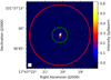 |
Fig. 1 ALMA 235.5 GHz continuum image of Sgr B2(M) at 0.4′′ angular resolution (Sánchez-Monge et al. 2017, from) with the FWHM HIFI beam at 480 (band 1a) and 1907 GHz (band 7b) shown as red and green circles, respectively. |
2 Observations and data reduction
The Herschel/HIFI guaranteed time key project HEXOS (Herschel/HIFI observations of EXtraOrdinary Sources, Bergin et al. 2010) includes full line surveys of Sgr B2(N) toward αJ2000 = 17h47m19.s88, δJ2000 = 28°22′ 18.′′ 4 and Sgr B2(M) toward αJ2000 = 17h47m20.s35, δJ2000 = 28°23′ 3.′′ 0, covering frequency ranges from 479.581–1280.148 GHz and 1444.999–1907.119 GHz at a spectral resolution of 1.1 MHz with corresponding half-power beam widths of 44.9–16.8′′ and 14.9–11.3′′, see Fig. 1.
Full spectral scans of HIFI bands 1a up to 7b toward Sgr B2(M) were carried out respectively on March 1, 2, and 5 2010, providing coverage of the frequency range 479 through 1907 GHz. HIFI spectral scans were carriedout in dual beam switch (DBS) mode, where the DBS reference beams lie approximately 180′′ east and west.
The spectral scans have been calibrated with HIPE version 10.0 (Roelfsema et al. 2012). The resulting double-sideband (DSB) spectra were reduced and deconvolved with the GILDAS CLASS2 package. For a detailed description of the calibration process see Schmiedeke et al. (2016, Sect. 2.1).
3 Data analysis
The survey was modeled using the eXtended CASA Line Analysis Software Suite (XCLASS3, Möller et al. 2017)with additional extensions (Möller in prep.). XCLASS enables the modeling and fitting of molecular lines by solving the 1D radiative transfer equation assuming local thermal equilibrium (LTE) conditions and an isothermal source
![Mathematical equation: \begin{align*}T_{\textrm{mb}}(\nu) =\;& \sum_{m,c \in i} \Bigg[\eta \left(\theta_{\textrm{source}}^{m,c}\right) \left[S^{m,c}(\nu) \left(1 - e^{-\tau_{\textrm{total}}^{m,c}(\nu)}\right)\right. \\ &\left.+ I_{\textrm{bg}} (\nu) \left(e^{-\tau_{\textrm{total}}^{m,c}(\nu)} - 1\right) \right] \Bigg]\nonumber\\ &+ \left(I_{\textrm{bg}}(\nu) - J_{\mathrm{CMB}} \right),\nonumber \end{align*}](/articles/aa/full_html/2021/07/aa40203-20/aa40203-20-eq1.png) (1)
(1)
where the sums go over the indices m for molecule, and c for component, respectively. Here, η(θm,c) indicates the beam filling (dilution) factor, Sm,c(ν) the source function, see Eq. (2), and  the total optical depth of each molecule m and component c. Furthermore, Ibg represents the background intensity and JCMB the intensity of the cosmic microwave background. In the following, we assume that the background intensity is equal to the intensity of the cosmic microwave background, that is Ibg ≡ JCMB. Under the LTE assumption, the kinetic temperature of the gas can be estimated from the rotation temperature: Trot ≈ Tkin. As these high-mass star-forming regions have high H2 densities nH_2 > 105 cm−3, LTE conditions can be assumed (Mangum & Shirley 2015). Line profiles are assumed to be Gaussian, but finite source size, dust attenuation, and optical depth effects are taken into account as well. Additionally, molecular parameters (e.g. transition frequencies, Einstein A coefficients, partition functions) are taken from an embedded SQLite database containing entries from the Cologne Database for Molecular Spectroscopy (CDMS, Müller et al. 2001, 2005) and Jet Propulsion Laboratory database (JPL, Pickett et al. 1998) using the Virtual Atomic and Molecular Data Center (VAMDC, Endres et al. 2016). In contrast to the standard CDMS, the database used by XCLASS describes partition functions for more than 1000 molecules between 1.07 and 1000 K, so extrapolation is no longer necessary for most molecules. The contribution of each molecule is described by multiple emission and absorption components, where each component is specified by the source size θsource, the rotation temperature Trot, the column density Ntot, the line width Δv, and the velocity offset from the systemic velocity voff. Additionally, each component can be located at a certain distance l along the line of sight. Moreover, XCLASS offers the possibility to fit these model parameters to observational data by using different optimization algorithms. The modeling can be done simultaneously with corresponding isotopologues and vibrationally excited states. The ratio with respect to the main species can be either fixed or used as an additional fit parameter.
In line-crowded sources like Sgr B2(M) line intensities from two neighboring lines, which have central frequencies with (partly) overlapping width regions, do not simply add up if at least one line is optically thick. Here, local line overlap has to be taken into account, where photons emitted from one line can be absorbed by the other line. The extended XCLASS package provides the possibility to take local line overlap (described by Cesaroni & Walmsley 1991) from different components into account, where we define an average source function Sl at frequency ν and distance l
 (2)
(2)
Here, εl represents the emission and αl the absorption function,  the excitation temperature, and
  the optical depth of transition t and component c, respectively. For each frequency channel ν, we take all transitions t into account which belong to the current distance l and whose Doppler-shifted transitions frequencies are located within a range of 5 Δvmax. Here, Δvmax describes the largest line width of all components located at the current distance. Additionally, the optical depths of the individual lines included in Eq. (1) are replaced by their arithmetic mean at distance l, that is
![Mathematical equation: \begin{equation*}\tau_{\textrm{total}}^{l}(\nu) = \sum_c \left[\left[ \sum_t \tau_t^c (\nu) \right] + \tau_{\textrm{d}}^{c} (\nu)\right], \end{equation*}](/articles/aa/full_html/2021/07/aa40203-20/aa40203-20-eq6.png) (3)
(3)
where the sums run over both components c and transitions t. Additionally, the dust opacity  is added as well. The iterative treatment of components at different distances, takes non-local effects into account as well. In the optically thin limit, Eq. (2) is equal to the traditional approach of describing a line as a sum of several Gaussians.
Extinction from dust is very important in the submillimeter and THz regime, particularly for a massive source like Sgr B2(M). In XCLASS, dust opacity of a component c is described using the equation
 (4)
(4)
Here,  describes the hydrogen column density (in cm−2),
  the dust mass opacity for a certain type of dust (in cm2 g−1, Ossenkopf & Henning 1994), and βc the spectral index. Additionally, νref = 230 GHz indicates the reference frequency for
  ,
,  the mass of a hydrogen molecule, and 1∕χgas-dust the dust to gas ratio which is set here to 1∕100 (Hildebrand 1983). The equation is valid for dust and gas well mixed.
For Sgr B2(M), we assume a two layer model where the first layer (hereafter called core-layer) describes contributions from the 27 continuum sources identified by Sánchez-Monge et al. (2017) and the second layer (envelope-layer) features located in the envelope. Here, we assume that all components belonging to a layer have the same distance to the observer. The source size used for the core layer is given by the angular size of the sum of solid angles of each core. For the envelope layer we assume beam filling, that is all molecules located in the envelope cover the full beam. For both layers we assume a dust mass opacity of κ1300 μm = 0.511 cm2 g−1 (agglomerated grains with thin ice mantles in cores; Ossenkopf & Henning 1994) and a spectral index of 1.6. The dust temperature and the hydrogen column density used for the core layer is derived from the 3D radiative transfer model presented in Schmiedeke et al. (2016) and is set to  K and
K and  cm−2, respectively. In order to obtain the remaining parameters for the envelope-layer, we fit the dust temperature and the column density,
  to the HIFI continuum, while we keep the other dust parameters fixed. We obtain a dust temperature of
  K and a column density of
  cm−2. In order to get a smooth continuum we subtracted the continuum from the data and add a synthetic dust continuum using the aforementioned dust model.
In the first steps of the analysis of the line survey, we estimate initial parameter sets for each molecule showing at least one transition within the HIFI survey using parameters from previous surveys of Sgr B2(M) and N (Belloche et al. 2013; Neill et al. 2014) and the new XCLASS GUI included in the extended XCLASS package. Here, we describe the continuum by the aforementioned two layer dust model. Furthermore, we assume that emission lines are modeled by components within the core layer, because these lines require in general excitation temperatures above the continuum level, which occur only in the hot cores. In contrast to that, absorption features are described by components located in the envelope layer, because here low excitation temperatures below the continuum level are needed. Additionally, some absorption lines have velocities far away from the source velocity of Sgr B2 and cannot originate from the cores. For species with complex line shapes like H2O or NH3, this assumption is no longer valid, because these molecules have to be described in Non-LTE, which is beyond the scope of this paper. Afteradjusting the parameters by eye we use the Levenberg-Marquardt algorithm to improve the description further. A molecule is claimed as identified if all lines in the survey range which have, based on the fit, an intensity higher than 3σ at the line frequency and are not blended, are detected with a line strength commensurate with the fit prediction. Additionally, we take N II (singly-ionized nitrogen), CH3OCH3 (dimethyl ether), NH2CHO (formamide), and N2O (dinitrogen monoxide) into account, although only weak lines below the 3σ level are observed. In order to model contributions of other species, we compute for each molecule the total spectrum caused by all other identified molecules and store the numerator εl and denominator αl of Eq. (2) representing the emission and absorption functions, respectively, as function of frequency ν and layer l. Afterwards, we repeat fitting each identified molecule, where we add the emission  and absorption
  functions describing the contributions from the other molecules to Eq. (2), that is
 (5)
(5)
to describe all other species as well. This procedure is repeated until the fit results show only minor changes.
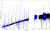 |
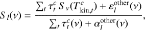
Fig. 2 Full view of the (uncorrected) Sgr B2(M) HIFI survey, where the HIFI bands are divided into “a” (blue) and “b” (black) bands) |
3.1 Isotope ratios
In order to simplify the comparison of our results with those derived by Neill et al. (2014), we used the same isotope ratios, that is set the 12C/13C ratio to 20, the 16O/18O to 250 and 32S/34S to 13. Additionally, we take the ratios described by Neill et al. (2014) for 16O/17O to be 800, for 32S/33S to be 75, for 14N/15N to be 182, and for 35Cl/37Cl to be 3. If deuterated isotopologues are identified, we leave the ratio as an additional fit parameter. Although some isotopic ratios are known to vary across the Galaxy, we kept the isotope ratios constant for all components along the line of sight because our main emphasis was a discussion of the lines originating in Sgr B2 itself.
3.2 Statistics of the HIFI spectrum
A spectral line is considered to be detected when the peak intensity exceeds the 3σ level of the random noise, which is calculated by first subtracting the continuum and applying astropy’s (Astropy Collaboration 2018) sigma-clipping algorithm to each band, respectively. Additionally, we only take into account those lines with line widths comparable to that of all other detected lines (5–40 km s−1), see Fig. 9. In this way one excludes single channel spikes, noise features, and other instrumental effects.
In order to determine the number of unidentified peaks, we use scipy’s (Virtanen et al. 2020) peak finding algorithm SCIPY.SIGNAL.FIND_PEAKS to identify peaks in the observational data. Additionally, we calculate for each peak the corresponding width. Somefeatures show a highly asymmetric line shape caused by contributions from neighboring lines or other species. In order to derive a reliable width, we determine the left and right line width, that is we use the interpolated positions of left and right intersection points of a horizontal line at the respective evaluation height of the peak. If both parts differ by less than a factor two, that is less asymmetric line shape, we take the sum of both parts as the final line width. But, if both parts differ by more than afactor of two, we use twice the smaller part as final line width. By calculating the line width in the aforementioned way, we reduce the number of erroneous line widths caused by line blending, see Fig. 4.
All features showing heights above the 3σ level and line widths which are comparable to that of all other detected lines, are compared with our model. Similar to Neill et al. (2014) for Sgr B2(N), we take a peak as unidentified, if the model for the corresponding feature is at least a factor of five weaker thanthe observed line intensity. The aforementioned method for emission lines is applied to absorption features as well, but here we have to start the identification process with the inverted spectrum to apply the scipy algorithm. As shown in Fig. 5, between 5 and 21% of all peaks in a single band are unidentified except for band 6a, where all peaks are identified. From this analysis, we estimate 1276 features (including both assigned and unassigned) in the Sgr B2(M) survey, where 14% are not identified, which is similar to the fraction of unidentified lines (≈8%) in Sgr B2(N) reported by Neill et al. (2014).
Some molecules show a superposition of different absorption components with systemic velocities distributed over a wide velocity range. Due to the differential rotation of the Milky Way, spectral features from clouds at different galactocentric radii can be associated with different velocity ranges, see (Whiteoak & Gardner 1979; Greaves & Williams 1994; Sofue 2006; Vallée 2008), which are described in Table 1. Streaming motions in the arms complicate the determination of the distance and hence the assignment to a specific spiral arm.
The integrated line intensities for each species are shown in Table 2. The values are derived from the best-fit LTE models, where we subtract the continuum before we integrate the spectra. Additionally, we compute the integrated line intensities for both core and envelope components as well as for different velocity ranges associated with different parts along the line of sight as described in Table 1. In order to compute the integrated intensity foreach spectral feature, we use the LTE parameters of the full model and take only those components into account which belong to the corresponding range. In doing so, we neglect contribution from other components, which may cause discrepancies between the sum of different parts and the total values, see Fig. 3.
Similar to Sgr B2(N) (Neill et al. 2014), methanol is the main contributor to the HIFI spectrum besides SO2. These two molecules together with CO also contribute the most (64.61%) to the core of Sgr B2(M). The envelope layer describing the envelope of Sgr B2(M) and other kinetic features along the line of sight, see Table 1 are dominated by ortho-H2O, CO and OH+. In general, ortho-H2O is the molecule with the strongest integrated intensity over all its transitions in any velocity range, except the envelope around Sgr B2(M), which consists mainly of CO, 13CO, and para-H2O. Additionally, ortho-H2O is not detected within the range between − 9 and 8 km s−1 associated with the Galactic center, which is dominated by ortho-H2O+ and OH+. The part of the Norma arm (−47 to −13 km s−1), which is covered by our observation, contains besides ortho-H2O mainly OH+, CH+, HF and NH. Similarly OH+ and CO are the molecules with the strongest integrated intensities across all their transitions, apart from ortho-H2O, in the Scutum arm (12–22 km s−1).
In general, complex molecules like NH2CHO (HC(O)NH2), CH3NH2 or CH3OCH3 exist only in the core of Sgr B2(M), while some simpler molecules/ions like ArH+ or 14N+, are clearly not associated with Sgr B2(M) but with the clouds and diffuse gas located throughout the Galactic arms. Additionally, all sulfur bearing molecules and their isotopologues contribute only to the cores, except SH+ and H2S. SH+ is mainly found in the envelope, but it is also distributed along the line of sight. In addition, all cyanide molecules except HCN, which is observed in the envelope as well, are identified only in the cores. In contrast, the detected halogen molecules HF, HCl, and H2Cl+ and hydrocarbons CH (except CH+ and CCH) appear only in the envelope. para-H2Cl+ shows a small contribution to the core layer as well. Most of the detected simple O-bearing and NH-bearing molecules are seen both in the core and in the envelope.
Finally, Table 2 can be used to identify the major molecular coolants in Sgr B2(M) within the frequency ranges covered with HIFI, which are shown in Fig. 6. Due to the fact that the gas can cool through emission of the photons, we take only the emission components into account. Additionally, contributions from absorption lines are ignored, because they only heat the gas when the energy of absorption is released via collisions, otherwise it is radiated (isotropically), that is in a certain sense it is only a scattering. Since the densities in the absorption components are expected to be much lower than the critical densities of the absorbing molecules, collisional deexcitation and therefore heating of the gas seems unlikely.
Velocity ranges corresponding to different kinematic components, taken from Lis et al. (2014).
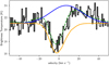 |
Fig. 3 Spectrum of the 1 837 816.8 MHz transition of OH. The full LTE model of OH (green dashed line) is superposed on the HIFIspectrum (black histogram). The contribution of the core and the envelope are shown as blue and orange lines, respectively. In order to determine the integrated intensities of different components and velocity ranges we take only those components into account, which belong to a specific range. By doing so we neglect the contributions from other components as shown here. The sum of integrated intensities of core and envelope contributions is about a factor two higher than the integrated intensity of the full LTE model. |
Integrated line intensities for each molecule in the model to the Sgr B2(M) spectral survey.
4 Results
In this section we describe the molecules and their isotopologues and vibrational excited states detected in the Sgr B2(M) HIFI survey, see Fig. 7. The derived LTE parameters are described in Tables A.1 and A.2. The detected molecules are divided into nine families (simple O-bearing molecules (Sect. 4.1), complex O-bearing molecules (Sect. 4.2), NH-bearing molecules (Sect. 4.3), N- and O-bearing molecules (Sect. 4.4), cyanide molecules (Sect. 4.5), S-bearing molecules (Sect. 4.6), carbon and hydrocarbons (Sect. 4.7), halogen molecules (Sect. 4.8), other molecules (Sect. 4.9)), which are defined by chemical relationships, for example, having the same heavy-atom backbone or the same functional group, and thus possibly related chemistry.
Since 12CO and ortho/para-H2O have extremely complex line shapes and their source geometry is too complex as well as their optical depths are too high to be described by our modeling approach, these two molecules are only considered by purely effective line shape fits to the spectrum.
In the following sections, the quantum number J = N + S + L refers to the total angular momentum of the molecule, where N, S, and L describe the rotation, electron spin, and electron orbital angular momentum quantum numbers, respectively. For species without an electronic angular momentum, that is J = N, the rotation transitions are indicated by ΔJ, while for species with electronic angular momentum the rotation levels are labeled as NJ. Symmetric rotor energy levels are described by JK, where K refers to theangular momentum along the symmetry axis. Energy levels for asymmetric rotors, are labeled as  , where Ka and Kc represent the angular momentum along the axis of symmetry in the oblate and prolate symmetric top limits, respectively.
A figure showing spectra of each detected molecule can be found in appendix4. For molecules with a large number of transitions, a representative sample of the detected transitions is shown.
A reliable estimation of the errors of the model parameters described in Tables A.1 and A.2 is not feasible within an acceptable time. We have therefore determined the errors of the four model parameters for CN as a proxy for the other parameters to give the reader some guidance on the reliability of the model parameters. (The error analysis of species with multiple temperature components can be different.) Here, we use again Eq. (5) to take the contributions of all other species into account. The errors were estimated using the emcee5 package (Foreman-Mackey et al. 2013), which implements the affine-invariant ensemble sampler of Goodman & Weare (2010), to perform a Markov chain Monte Carlo (MCMC) algorithm approximating the posterior distribution of the model parameters by random sampling in a probabilistic space.
The MCMC algorithm starts at the estimated maximum of the likelihood function, that is the model parameters of CN described in Tables A.1 and A.2, and draws 46 samples (walkers) of model parameters from the likelihood function in a small ball around the a priori preferred position. In the following, 100 burn-in steps are performed to let the walkers explore the parameter space. Afterwards, we used further 200 steps to sample the posterior.
After finishing the algorithm the probability distribution and the corresponding highest posterior density (HPD) interval of each free parameter iscalculated. A HPD interval is basically the shortest interval on a posterior density for some given confidence level, that is 68% for 1σ, 95.4% for 2σ etc. For the error estimation of CN, we are considering a 1σ (68%) confidence interval, that is the HPD interval is the shortest interval that contains 68% of the probability of the posterior. In order to compute a HPD interval we rank-order the MCMC trace. We know that the number of samples included in the HPD is 0.68 (or another confidence level) times the total number of MCMC samples. Therefore, we consider all intervals containing these many samples and find the shortest interval. In the case of a normal distribution,an HPD interval coincides with the usual probability range, which is symmetric about the mean and includes the quantiles  and
and  . So, the error estimation algorithm reports the (first) mode and then the bounds on the HPD intervals. Here, the mode must not coincide with the best fit result of the previously applied algorithms.
The posterior distributions of the individual parameters of CN are shown in Fig. 8. For all histograms we find a unimodal distribution, that is there is only one best fit within the given parameter ranges.
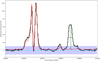 |
Fig. 4 Example of unidentified peaks in the HIFI survey of Sgr B2(M) in band 1b. The observed spectrum is shown in black, the full model in red, and the cyan dashed line marks the continuum level. The blue area represents the + ∕−3σ level, i.e., all peaks that do not protrude from this area are ignored. The height and width of the unidentified feature near 620.7 GHZ is described by the horizontal and vertical green line, respectively. The peaks indicated by the small gray vertical lines are ignored, because their line widths are below the lower limit of the allowed range of line widths. |
 |
Fig. 5 Fraction of unidentified peaks as function of band. |
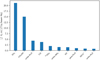 |
Fig. 6 Ten strongest cooling molecules in Sgr B2(M) in the frequency ranges covered with HIFI. |
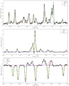 |
Fig. 7 Excerpts of the HIFI survey of Sgr B2(M) in bands 1a and 3b (solid black line), with the full model (dashed green line) and those of the molecules contributing to the spectral range of each panel. |
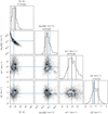 |
Fig. 8 Corner plot (Foreman-Mackey 2016) showing the one and two dimensional projections of the posterior probability distributions of the model parameters of CN. On top of each column the probability distribution for each free parameter is shown together with the value of the best fit and the corresponding left and right errors. The left and right dashed lines indicate the lower and upper limits of the corresponding HPD interval, respectively. The dashed line in the middle indicates the mode of the distribution. The blue lines indicate the parameter values of the best fit. The plots in the lower left corner describe the projected 2D histograms of two parameters and the contours the HPD regions, respectively. In order to get a better estimation of the errors, we determine the error of the column density on log scale and use the velocity offset (voff) related to the source velocity of vLSR = 64 km s−1. |
4.1 Simple O-bearing molecules
CO
Carbon monoxide (CO) and its five isotopologues 13CO, C17 O, C18 O, 13C17O, and 13C18O are clearly identified, see Figs. B.1–B.6. The vibrational excited states CO, v = 1 and CO, v = 2 are not detected. The energetically low lying transitions of CO up to Jup = 7 have a P Cygni line shape with additional strong red-shifted absorptions at 21 and 78 km s−1. Additionally, transitions up to Jup = 13 show an inverse P Cygni line shape, whereas transitions with higher J as well as all transitions of the five isotopologues are seen in pure emission.
CH3OH
Methanol (CH3OH) is detected through a large number (351 features with intensities above the 3σ level) of transitions ranging from the ground state to energies of about 1000 K, see Fig. B.7. Methanol contributes strongly to the HIFI spectrum and the interaction of torsional and rotational motions leads to multiple energy states and a complex spectrum, which is described by a cold (Trot = 39 K) and three warm emission (Trot = 89–308 K) in conjunction with two cold absorption (Trot = 2–10 K) components. Compared to Sgr B2(N) (Neill et al. 2014), we detect fewer absorption components but use a cold (Trot = 39 K) and warm (Trot = 308 K) emission component, which might be caused by the fact that the entry for methanol in the database has been extended considerably in J, K, vt, and in frequency since 2014 and is now based on Xu et al. (2008). The 13CH3OH isotopologueis also fit by the same model, see Fig. B.8.
H2CO
Transitions of ortho- and para-formaldehyde (H2CO) have been detected in emission, see Figs. B.9 and B.10. The contribution of ortho-H2CO is fitted by two warm emission components (Trot = 44–68 K), whereas para-H2CO requires slightly higher temperatures (Trot = 45–74 K).
HCO+
In good agreement to Sgr B2(N) (Neill et al. 2014), the energetically low lying transitions of formyl radical (HCO+), ranging from Jup = 6–14, are clearly observed, see Fig. B.11. Transitions up to Elow = 282.4 K show self-absorption. The isotopologues H13 CO+ (Fig. B.12) and HC18O+ (Fig. B.13) are clearly identified, whereas neither HC17O+, nor DCO+ nor vibrational excited states are seen in the HIFI survey.
HOCO+
Protonated carbon dioxide (HOCO+) is identified through absorption transitions, see Fig. B.14, which are, in agreement with Sgr B2(N) (Neill et al. 2014), well described by two cold (Trot = 6–7 K) components. The isotopologue HO13CO+ is not clearly observed.
OH
Congruent with Goicoechea & Cernicharo (2002), we also clearly observe intra-ladder rotational transitions (2 Π1∕2J = 3∕2+ −−1∕2−) of hydroxyl (OH) near 1835 and 1838 GHz, see Fig. B.15. But in contrast to Goicoechea & Cernicharo (2002) and opposed to observations of Sgr B2(N) (Neill et al. 2014), OH shows self-absorption around these frequencies, which is well described by a warm (Trot = 241 K) emission and a cold (Trot = 30 K) absorption component. Since OH shows only two transitions within the HIFI survey with nearly the same lower energy (Elow = 181.707−181.935 K), the temperatures can not be determined and we had to assume the temperatures mentioned above to get a proper description.
OH+
The ground-state transitions (N = 1–0) of the hydroxyl radical (OH+) are seen in broad and deep absorptions ranging from −116 up to 66 km s−1, see Fig. B.16. Neither higher excited lines nor its isotopologues OD+ and 18OH+ are detected.
H2O
Observations of fundamental rotational transitions of ortho- and para-H O and H
 O in absorption are partly described in Lis et al. (2010), see Figs. B.17, B.18, B.21, and B.22. Additionally, as already described by Comito et al. (2010), the ground state and the 21,2 –10,1 transition ofHDO was observed in absorption, see Fig. B.23, whereas higher excited lines up to Elow = 66.4 K are seen in emission. Furthermore, we detect the ground-state transitions of ortho- and para-H
 O in absorption around 64 km s−1, Figs. B.19, B.20. For ortho-H
 O, we do not see higher excited lines except the 31,2 –30,3, and 32,1 –31,2-transitions, which are observed in emission. For para-H
 O, we detect the next two excited states, which are closest to the ground state in emission. The ground-state transition of ortho-H
 O is not clearly observed, because it is strongly blended by the para-H2O+ transition at 607 GHz. Neither D2O nor vibrationally excited states are observed except for H2O, v2 = 1, where we see a line at the correct frequency (658 GHz), but it cannot fit together with the other water lines because it probably originates from a very small, very hot region.
H2O+
The detection of ground-state transitions ( = 110 –101) of ortho- and para-oxidaniumyl (H2O+) in the HIFI survey was previously described by Schilke et al. (2010), see Figs. B.24, B.25, with slightly different parameters caused by our extended dust model.
H3O+
As already described in Lis et al. (2014), metastable inversion transitions of hydronium (H3O+) are observed in the HIFI survey, see Figs. B.26, B.27. We clearly identified the ground-state, the 3 –3
–3 , and 4
 –3
–3 transitions of ortho-H3O+, where the energetically lowest states are seen in absorption while the transition at 1031 GHz is observed in emission. The contribution of ortho-H3O+ is well described by one cold emission (Trot = 39 K) and seven cold absorption components (Trot = 12–28 K). Although ortho-H3O+ has 20 transitions within the HIFI survey, it shows only one emission feature within the HIFI range, thus the temperature of the emission component is not well constrained and should be considered only as an upper limit. Additionally, we detect the ground-state, the 2
 –2
–2 , and 2
 –2
–2 transitions of para-H3O+ in absorption and use three cold components with excitation temperatures between 5 and 31 Kto model the contribution. Lis et al. (2014) derived temperatures of Trot = 177 ± 54 K and Trot = 546 ± 80 K for H3O+ using a combination of Gaussian fits and rotational diagrams but without distinguishing between ortho and para states. Moreover, Lis et al. (2014) consider only metastable levels of H3O+, that can be well described in LTE. However, we take all transitions into account, including those lines which are very far from LTE.
SiO
In contrast to Sgr B2(N) (Neill et al. 2014), the energetically low lying transitions (Jup = 12–18) of silicon monoxide (SiO) are clearly observed in emission, see Fig. B.28, and modeled with a cold (Trot = 25 K) and a warm (Trot = 104 K) component. Our temperatures agree quite well with those derived by Belloche et al. (2013) for their emission components. Other isotopologues or vibrationally excited states could not be identified.
4.2 Complex O-bearing molecules
CH3OCH3
As in previous line surveys Winnewisser & Gardner (1976); Cummins et al. (1986); Nummelin et al. (1998); Fuchs et al. (2005); Belloche et al. (2013); Neill et al. (2014) CH3OCH3 (dimethyl ether) is detected in weak lines, see Fig. B.29, although a large number of transitions is included in the survey. Similar to Neill et al. (2014) we used a single warm (Trot = 100 K) component to describe CH3OCH3 in Sgr B2(M).
Others
In contrast to other line surveys (Turner 1991; Nummelin et al. 1998; Friedel et al. 2004; Belloche et al. 2013) HCOOH (formic acid), H2CCO (ketene), C2H5OH (ethanol), vinyl cyanide (C2H3CN), ethyl cyanide (C2H5CN), and methyl formate (CH3OCHO) are not conclusively detected.
4.3 NH-bearing molecules
CH3NH2
Unlike in Sgr B2(N) (Neill et al. 2014), where CH3NH2 (methylamine) was clearly detected, we found only a weak detection from the cores, see Fig. B.30. Most of the lines are well described by a single component with an excitation temperatureof Trot = 14 K in contrast to Belloche et al. (2013) which used an emission (Trot = 50 K) and a cold absorption component (Trot = 2.7 K).
CH2NH
In contrast to Turner (1991) and Belloche et al. (2013), we see CH2NH (methylene imine) only in absorption in the envelope with a quite low excitation temperature of Trot = 11 K, see Fig. B.31. For Sgr B2(N), Neill et al. (2014) found CH2NH within the cores (Trot = 150 K) and within the envelope (Trot = 6–11 K). The isotopologues 13CH2NH and CH NH2 could not be detected.
NH
Similar to Sgr B2(N) (Neill et al. 2014) and in good agreement with Polehampton et al. (2007) and Etxaluze et al. (2013), three broad absorption features around 946, 974, and 1000 GHz have been clearly identified as hyperfine transitions ((J = 0, N = 1) ← (J = 1, N = 0), (J = 2, N = 1) ← (J = 1, N = 0), (J = 1, N = 1) ← (J = 1, N = 0)) of NH (nitrogen monohydride) with excitation temperatures between 5 and 14 K, see Fig. B.32.
NH2
The amino radical (NH2) is clearly identified within the core and the envelope, see Figs. B.33 and B.34. As in Sgr B2(N) (Neill et al. 2014), we see the 111 –000, 202 –111 and 313 –202 transitions of ortho-NH2 as well as the 212 –101 transitions of para-NH2 in absorption, while higher-energy transitions are seen in emission. Especially, the 211 –202 ortho-transitions show strong emission features.
NH3
Ammonia (NH3) is found in absorption in the envelope and in line of sight clouds, see Figs. B.35 and B.36. In contrast to Sgr B2(N) (Neill et al. 2014), the ground-state transition (J = 0, K = 1) ← (J = 0, K = 0) near 572 GHz of ortho-NH3 shows self-absorption around 64 km s−1. The higher-excited transitions (J = 2, K = 0) ← (J = 1, K = 0) and (J = 3, K = 0) ← (J = 2, K = 0) at Elow = 28 and 86 K are seen in absorption only. All three observed transitions show multiple absorptions from −149 to 65 km s−1. Additionally, we detect ground state and energetically low lying transitions of para-NH3 up to Elow = 58 K in absorption, where the three energetically lowest transitions show multiple absorptions between −103 and 64 km s−1. Neither the ortho nor the para form of 15NH3, NH2D, NH3D+, ND3, and NH3,v2 = 1 could be detected.
N2H+
In contrast to Belloche et al. (2013) and in good agreement with Sgr B2(N) (Neill et al. 2014), we see the dyazenilium ion (N2H+) only in emission through four transitions, from Jup = 6 to 9, see Fig. B.37. Its isotopologues N2D+, 15NNH+, N15NH+, 15NND+, N15ND+ and the vibrational state N2H+,v2 = 1 could not be identified.
N+
As in Sgr B2(N) (Neill et al. 2014), the fine-structure transition (2P1–2P0) of the single ionized atomic nitrogen [N II] at 1461.1 GHz is identified in absorption around 64 km s−1, see Fig. B.38. In contrast to Etxaluze et al. (2013), we can not find [N II] in emission.
4.4 N- and O-bearing molecules
HNCO
As in previous line surveys (Sutton et al. 1991; Nummelin et al. 1998; Belloche et al. 2013) we also see isocyanic acid (HNCO) in Sgr B2(M), see Fig. B.39. All b-type transitions between the Ka = 0 and 1 ladders, in the P (ΔJ = −1), Q (ΔJ = 0), and R (ΔJ = +1) branches, are observed in this survey up to J = 17. Caused by the strong continuum in the far-infrared, these lines are all observed in absorption. Similar to Sgr B2(N) (Neill et al. 2014), we use three cold (Trot = 13–17 K) absorption components with slightly different velocities, which is consistent with Churchwell et al. (1986), who found a rotational temperature of 10 K for transitions with Elow < 40 K in the millimeter (Ka = 0 a-type transitions). Like in Sgr B2(N), we also detect high-energy (Jup = 22) a-type transitions in emission with lower-state energies ranging from 300–900 K, originating from the cores. In agreement with Neill et al. (2014) and in contrast to Belloche et al. (2013), we use a single core component with a rotational temperature of 300 K to describe these emissions.
Additionally, we also identified the Ka = 1–0 Q branch of HN13CO, see Fig. B.40. Due to the fact that the carbon nucleus is located very near the center of mass of the molecule, the change of the B and C rotational constants from HNCO to HN13CO (δB∕B and δC∕C ~ 3 × 10⁻⁵) is very small. Therefore, a-type transitions of HN13CO are blended with their HN12CO counterparts. However, the A rotational constant changes by ~2 GHz between isotopologues, which shifts the b-type transitions in frequency and thus allows their detection. Other isotopologues like H15NCO, HNC17O, or HNC18O are not detected.
NH2CHO
A-type (μa = 3.61 debye) and b-type (μb = 0.85 debye) transitions of formamide (NH2CHO or HC(O)NH2) are only weakly detected in emission, in contrast to Sgr B2(N) (Neill et al. 2014). Although the HIFI bandwidth covers an enormous number of transitions up to Jup = 92 we see only the 232,21–222,20, 242,22–232,21,262,24–252,23, and 272,25–262,24 transitions, which are well described with a single hot component (Trot = 300 K), see Fig. B.41.
NO
Similar to Sgr B2(N) (Neill et al. 2014), Nitric oxide (NO) is clearly identified through a large number of transitions in emission, see Fig. B.42. The lines are well described by a cooler (Trot = 25 K), warmer (85 K), and hotter (325 K) components which are associated with the hot core. Its isotopologues 15NO, N17O, N17O, N18O, and 15N17O are not seenin the HIFI survey.
HNO
The three low-energy transitions 111 –000, 212 –101, and 110 –101 of HNO (nitroxyl) are detected in absorption from the Sgr B2(M) envelope, see Fig. B.43.
N2O
In agreement with Nummelin et al. (1998), N2O (dinitrogen monoxide) is identified in emission through nine transitions, from Jup = 20–29, see Fig. B.44.
4.5 Cyanide molecules
HCN
Hydrogen cyanide (HCN), its isotopologues (H13CN), and the vibrational excited state HCN, v2 = 1 are clearly observed both in emission and absorption, see Figs. B.45–B.47, and already described in Rolffs et al. (2010).
HNC
Like in Sgr B2(N) (Neill et al. 2014), the energetically low lying transitions of isocyanide (HNC) up to Jup = 12 are observed, see Fig. B.48. Its isotopologue HN13C is also detected, see Fig. B.49. Similar to HCN, we also observe the vibrationally excited state HNC, v2 = 1, see Fig. B.50.
CH3CN
Methyl cyanide (CH3CN) is observed in many transitions with lower energies up to Elow ~ 1200 K, see Fig. B.51. In contrast to other observations (de Vicente et al. 1997; Belloche et al. 2013; Araki et al. 2020), we see CH3CN only in emission, which can be fit well with a single hot component. An additional second component, as used for Sgr B2(N) (Neill et al. 2014), is not necessary. The derived rotational temperature of Trot = 187 K, correspondsquite well to the temperature of the emission component (Trot = 200 K) described by Belloche et al. (2013). The absence of absorption features in the HIFI survey is caused by the fact, that the energetically lowest transition of CH3CN has a lower energy of Elow = 310 K well above the continuum level. Neither the 13C, nor the 15N isotopologues, nor the rotational transitions in the ν8 = 1 state are detected.
CN
The energetically lowest hyperfine transitions (Elow ≤ 152 K) near 566, 680, 793, and 907 GHz of the cyano radical (CN) are clearly observed in emission, see Fig. B.52. In agreement with Belloche et al. (2013) and Neill et al. (2014) (for Sgr B2(N)), we use a single cold component with a slightly lower temperature of Trot = 34 K. Absorptions, as described by Belloche et al. (2013), are not seen. The isotope 13CN is also detected in emission, see Fig. B.53.
HCCCN
In opposite to Sgr B2(N) (Neill et al. 2014), we clearly observe the energetically low lying transitions (Elow ≤ 672.2 K) of cyanoacetylene (HCCCN), see Fig. B.54. We use, (in good agreement with Goldsmith et al. 1987; Sutton et al. 1991; Belloche et al. 2013), a cold (Trot = 31 K) and a warm component (Trot = 90 K) to describe the contribution of HCCCN to the HIFI spectrum. Neither its isotopologues (H13CCCN, HC13CCN, HCC13CN, HCCC15N, DCCCN, D13CCCN, DC13CCN, DCC13CN, DCCC15N, H13C13CCN, H13CC13CN, HC13C13CN, HC13CC15N) nor vibrationally excited states are detected.
4.6 S-bearing molecules
H2S
In good agreement to Tieftrunk et al. (1994), we clearly detected hydrogen sulfide (H2S) and its isotopologues H S and H
 S in emission and absorption, see Figs. B.55–B.60. In contrast to Sgr B2(N), the ground-state transition (212 –101) of ortho-H2S shows self-absorption and a series of cold, red-shifted absorptions with velocities down to −104 km s−1. Even the ground-state transitions of both isotopologues show a combination of red-shifted emission and blue-shifted absorption features. Higher energy transitions are observed only in emission, except the (221 –110) transition (Elow = 8.1 K) of ortho-H2S, which shows self-absorption. para-H2S and its isotopologues para-H
 S and para-H
 S are identified as well, whereas para-H
 S is only weakly detected. All transitions are seen in emission, except the (202 –111) and (313 –202) transitions of para-H
 S which show self-absorption as well. (Opposed to ortho-H2S, the ground state transition of para-H2S is not included in the HIFI survey.)
SO
Sulfur monoxide (SO) is identified in emission, see Fig. B.61. Similar to Sgr B2(N) (Neill et al. 2014), we use four components to describe the contribution of SO, where the two hot components have comparable temperatures (Trot = 169–174 K). But unlike Sgr B2(N) and in good agreement with Belloche et al. (2013), we use two cold (Trot = 17–28 K) instead of two warm components. The weaker 34SO lines are modeled with two warm components, see Fig. B.62. The other isotopologues 33SO, 36SO, S17O, S18O, are not detected.
SO2
Sulfur dioxide (SO2) is clearly detected in emission, see Fig. B.63, and well described by three cold (Trot = 15–34 K), one warm (Trot = 69 K), and two hot components (Trot = 500 K). Its isotopologues 33SO2 and 34SO2 are also observed, see Figs. B.64 and B.65, but SO17O and SO18O and the vibrational excited state SO2, v2 = 1 are not conclusively detected.
CS
Rotational transitions of carbon monosulfide (CS) up to Jup = 22 (Elow = 542.7 K) are detected, see Fig. B.66, but in contrast to other line surveys (Belloche et al. 2013; Neill et al. 2014) only in emission. We use two warm components (Trot = 41–99 K) to model the contribution of CS. The isotopologues 13CS, C33S, C34S are also clearly observed, see Figs. B.67 and B.69, whereas the vibrational excited states CS, v = 1, CS, v = 2, CS, v = 3, and CS, v = 4 are not seen.
H2CS
In agreement with Sgr B2(N) (Neill et al. 2014), thioformaldehyde (H2CS) is weakly observed in emission, see Fig. B.70, and modeled with a single warm component (Trot = 120 K). A low temperature contribution as described by Belloche et al. (2013) is not seen.
OCS
Comparable to Sgr B2(N) (Neill et al. 2014), all transitions of carbonyl sulfide (OCS) ranging from Jup = 40–60 (Elow = 455–1032 K) are observed, see Fig. B.71 in emission and well described by two warm components (Trot = 135–173 K) with slightly different velocity offsets (voff = 57.5–66.5 km s−1). The isotopologues 17OCS, 18OCS, O13CS, OC33S, OC34S, OC36S, O13C33S, O13C34S, 18O13CS, and 18O13C34S are not reliably detected.
HCS+
In contrast to Sgr B2(N) (Neill et al. 2014), transitions of thiomethylium (HCS+) are weakly observed in emission and modeled by a single warm (Trot = 51 K) component, see Fig. B.72.
NS
Similar to Sgr B2(N) (Neill et al. 2014), nitrogen sulfide (NS) is clearly detected in emission, see Fig. B.73. But in contrast to Belloche et al. (2013) we use a colder emission component (Trot = 70 K) describing the lower-energy (Ω = (1/2)) ladder, and do not see any absorption lines of NS, which is caused by the fact that the energetically lowest transition within the HIFI survey has Elow = 110 K. Neither the 15NS nor the N33S, nor the N34S isotopologues are seen.
SO+
Similar to Nummelin et al. (1998), we clearly identify the sulfoxide ion (SO+) in emission, see Fig. B.74. The detected transitions (20/2–18/2(f) to 39/2–37/2(e)) have lower energies from 110 to 400 K and are well described by two warm components (Trot = 50–90 K).
SH+
Consistent with Menten et al. (2011), we also observed sulfoniumylidene (or sulfanylium) (SH+) in absorption, see Fig. B.75. The ground-state transitions (12 –01 and 11 –01) at 526 and 683 GHz are seen with multiple velocity components between −144 and 66 km s−1, whereas the higher-excited lines (23 –12 and 21 –10) at 1083 and 1231 GHz are described by only a few velocity components around 64 km s−1. Additionally, we observed the ground-state transitions of 34SH+ in absorption, see Fig. B.76.
4.7 Carbon and hydrocarbons
CCH
We observe ethynyl (CCH) emission toward the hot cores and detect transitions from N = 6 – 5 to 21 – 20 (Eup = 63–879 K), see Fig. B.77. The doublets, caused by the unpaired electron, are clearly separated in the survey and well described by a single component without a red-shifted wing as described by Belloche et al. (2013). In contrast to Neill et al. (2014) we use a lower excitation temperature of Trot = 27 K with an order of magnitude higher column density of Ntot = 6.4 × 1015 cm−2. Neither the isotopologues C13CH, CC13H, and CCD nor the vibrational excited states CCH, v2 = 1, CCH, v2 = 2, and CCH, v3 = 1 could be detected reliably.
CH
In addition to the six hyperfine components of CH (methylylidene radical) in the ground electronic state (X 2 Π), (J = 3/2, N = 1) ← (J = 1/2, N = 1) near 532.8 and 536.8 GHz described by Qin et al. (2010), we observe the lowest transitions in the F1 ladder (J = 5/2, N = 2) ← (J = 3/2, N = 1) at 1657.0 and 1661.1 GHz, see Fig. B.78. But in contrast to the ground-state transitions which are seen with multiple velocity components between −93 and 65 km s−1, the higher-energy transitions are described by a few velocity components around 64 km s−1. In contrast to the isotopologue 13CH, which is clearly identified, see Fig. B.79, the vibrational excited state CH,v = 1 is not observed.
CH+
As in Sgr B2(N) (described by Godard et al. 2012; Neill et al. 2014) the methylylidene ion (CH+) and its isotopologue 13CH+ are clearly detected, see Figs. B.80, B.81. Similar to CH, the energetically low lying (J = 1–0) transition is seen with multiple velocity components between −128 and 73 km s−1, whereas the next rotational transition (J = 2–1) at 1669.2 GHz is centered around 64 km s−1. Additionally, we observe CD+ but only two transitions are located within the HIFI survey, so that we are not able to derive reliable physical parameters, see Fig. B.82.
C
Similar to Sgr B2(N) (Etxaluze et al. 2013; Neill et al. 2014) the neutral atomic carbon [C I] and its isotopologue 13C are clearly identified as well, see Figs. B.83, B.84. The 3P1–3P0 transition at 492 GHz and the 3P2–3P1 transition at 809 GHz are modeled by multiple components within the core and the envelope layer.
C+
Due the fact that only one transition, the 2P3∕2–2P1∕2 fine structure transition at 1901 GHz, is included in the HIFI survey, a reliable quantitative description of the single ionized atomic carbon was not possible, see Fig. B.85. As reported by (Neill et al. 2014) for Sgr B2(N), we also see [C II] in multiple absorption features around 64 km s−1.
C3
As reported by Goicoechea et al. (2000); Cernicharo et al. (2000); Polehampton et al. (2007); Neill et al. (2014) we also see vibrational excited transitions of the nonpolar linear carbon trimer, C3 in absorption around 64 km s−1, see Fig. B.86. The rovibrational Q(12), Q(10), Q(8), Q(6), Q(4), Q(2), P(4), and P(2) transitions are well described with two cold components with excitation temperatures of Trot = 8–10 K, in good agreement with Cernicharo et al. (2000); Giesen et al. (2020). But we need an additional warm component with Trot = 46 K to describe absorptions with lower-state energies ranging from 26–68 K. Energetically lower lying transitions of the Q band were not detected.
4.8 Halogen molecules
HF
The detection of (J = 1) ← (J = 0) transition ofHF (ethynyl radical) at 1232 GHz in the HIFI survey was previously described by Monje et al. (2011), see Figs. B.87, with slightly different parameters caused by our extended dust model. Its isotopologues DF is not detected.
HCl
As in Sgr B2(N) (described by Neill et al. 2014) we clearly detect the (J = 1–0) and (J = 2) ← (J = 1) hyperfine transitions of H35Cl (hydrogen chloride) and its isotopologue H37Cl, see Figs. B.88 and B.89. The transitions are modeled with five velocity components between 19 and 68 km s−1 and a mean column density of Ntot = 9.8 × 1013 cm−2, which is in good agreement with the column density of Ntot = 1.63 × 1014 cm−2 derived by Zmuidzinas et al. (1995).
H2Cl+
In agreement to Sgr B2(N) (described by Neill et al. 2014) H2Cl+ (chloronium) is clearly detected in Sgr B2(M) as well, see Figs. B.90, B.91. Here, we modeled the ortho and para form separately, where both states are described by Ka + Kc being odd and even, respectively.
4.9 Other molecules
ArH+
The detection of ArH+ (argonium) in the HIFI survey was previously described by Schilke et al. (2014). We derived slightly different parameters due to our differentmodeling method, see Fig. B.92.
5 Discussion
5.1 Physical parameters for molecular families
In order to visualize the distribution of the derived physical parameters we computed normalized kernel density estimations (KDE Rosenblatt 1956; Parzen 1962) for the fitted parameters of the different families introduced in Sect. 4, which are presented in Fig. 9, where we take all detected molecules and their isotopologues into account. (In the following we exclude CH3OCH3 and ArH+ because their respective families contain only one molecule). The KDE is a nonparametric way to estimate the probability density function of a given parameter and gives the most probable parameter value(s) for each parameter and molecular family. Additionally, it offers a visual representation of the individual parameters with the aim to see their spread and to search for general trends6. This is usually not easy to accomplish by just looking at numbers.
For the excitation temperatures we find mostly bimodal KDEs, presented in panels Figs. 9a and e, for all molecular families and for the total distribution of all molecules. The majority of the KDEs have two maxima around 20 and 500 K. For halogen molecules both maxima are shifted to 3 and 33 K, respectively,because these molecules appear only in the envelope and in clouds along the line of sight, except para-H2Cl+, which has one weak core component. Furthermore, the KDE for carbon and hydrocarbons shows even three local maxima at 8, 42, and 76 K, which might be caused by the fact that these molecules are mostly located in the envelope and in foreground clouds. The KDEs of the other families have their second maxima at higher temperatures, because these families contain molecules which are predominantly associated with the core of Sgr B2(M). The strong maximum at low temperatures appearing in all KDEs is due to the fact that the hot cores cover only a small fraction of the large HIFI beam. Therefore, molecules contained in the cold envelope dominate the HIFI spectrum. Similar to that, most of the column density KDEs, see Figs. 9b and f, show unimodal distributions, with a maximum around 1 × 1014 cm−2 for each family of molecules. Only the KDE for carbon and hydrocarbons have a second pronounced maximum at around 1 × 1018 cm−2. Additionally, the line width KDEs, shown in panels Figs. 9c and g, of most molecular families are rather unimodal with minor side maxima. The most abundant line width is around 9 km s−1, with a side maximum around 29 km s−1. Finally, the distribution of the velocity offsets, described in panels Figs. 9d and h, nicely fits to the velocity ranges (gray areas) associated with structures along the line of sight, see Table 1.
In Fig. 10, the abundances of all detected species associated with each family are shown in separate panels, using an H2 column density of 1.1 × 1024 cm−2 for the core and 1.8 × 1024 cm−2 for envelope components, respectively. The abundances we quote are source-averaged abundances. It is possible that a given molecule exists only in a subvolume of the core as seen by Herschel – either along the line of sight, or within the beam. Therefore, the local abundances can deviate from the values determined here. This property is due to finite spatial resolution. Unresolved substructure is most likely present in all but a few sources (for an example of substructure in a simple core see Friesen et al. 2014), which makes it a common trait of line surveys. The only way to improve this further is analyzing higher resolution data (Sánchez-Monge et al. 2017; Möller, in prep.). This is outside the scope of the present paper, and of course even then there may be variations on a scale unresolved by the beam. Additionally, we compare the abundances with those derived by Neill et al. (2014) for Sgr B2(N), which were obtained, reduced and analyzed with similar methods, so that observation and modeling effects are minimized. Nevertheless, the two analyses differ fundamentally in some points, which is why the results cannot be compared without limitations. In contrast to Neill et al. (2014), we take dust attenuation within the envelope into account, which leads to different hydrogen column densities, that is our column density of the core layer is about seven times lower than the one used by Neill et al. (2014) for Sgr B2(N). However, the results cannot be directly compared, since we take local-overlap effects into account, which is important for line crowded sources like Sgr B2(M) and N. Furthermore, for some molecules we distinguish between ortho and para states, see Sect. 5.2, which makes a direct comparison difficult. In the following, we discuss similarities and differences between the molecular abundances in the cores of Sgr B2(M) and Sgr B2(N) for each molecular group.
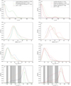 |
Fig. 9 Normalized KDE for different model parameters and molecule families defined in Sect. 4. Additionally, the bandwidth h of all KDEs used for each molecule family is given as well. The gray areas in d indicate the velocity ranges described in Table 1. The families “complex O-bearing molecules” (Sect. 4.2) and “other molecules” (Sect. 4.9) are not shown, because they contain only one molecule, respectively. |
O-bearing species
The abundances of simple and complex oxygen-bearing species are shown in Figs. 10a and b, respectively, where the abundance of some molecules (NH3 and H3O+) are influenced by the underlying LTE assumption. It is generally assumed that O- and C-bearing molecules have a common grain surface origin from the hydrogenation of CO on grain surfaces (see e.g., Fuchs et al. 2009; Garrod & Pauly 2011; Garrod 2013). Here, methanol is 19 times more abundant in Sgr B2(N), while Sgr B2(M) is richer in the formyl radical (HCO+). The abundance of dimethyl ether (CH3OCH3) in our survey is more than 77 times lower than for Sgr B2(N). Ignoring molecules, which have to be described in Non-LTE, we derive total abundances of 7.18 × 10⁻⁸ and 2.22 × 10⁻⁷ for all oxygen-bearing species within the core and envelope of Sgr B2(M), respectively.
NH-bearing species
Abundances of NH-bearing species are shown in Fig. 10c. In contrast to Sgr B2(N), methanamine (CH2NH) is not detected in the core, which makes a direct comparison difficult. Methylamine (CH3NH2) is more abundant in Sgr B2(N), while Sgr B2(M) contains more dyazenilium (N2H+). The abundances for both species differ by a factor of 7. The description of ammonia might be complicated by Non-LTE effects. The total abundances for NH-bearing species within the cores of Sgr B2(M) (excluding NH3) is 1.10 × 10⁻⁸. For the envelope of Sgr B2(M) we get 1.30 × 10⁻⁷, which is caused by the strong absorption lines of ammonia and the amino radical.
N- and O-bearing species
In Fig. 10d, the abundances of N- and O-bearing species are described. Here, the more complex molecules formamide (NH2CHO or HC(O)NH2) and isocyanic acid (HNCO) show a much higher abundance in Sgr B2(N) than in M. The enhancement varies between 13 for HNCO and 133 for formamide. Opposed to that, the abundance of nitric oxide (NO) is nearly the same in both sources. The total abundance in the core of Sgr B2(M) is 1.41 × 10⁻⁷ and 1.04 × 10⁻⁹ in the envelope, respectively.
CN-bearing species
The abundances of CN-bearing species are presented in Fig. 10e. Similar to the N- and O-bearing species, the more complex CN-bearing species ethyl cyanide (CH3CN) is more abundant in Sgr B2(N) compared to M, while the lighter molecules isocyanide (HNC) and cyano radical (CN) have a higher abundance in Sgr B2(M). The comparison of HCN must be considered with caution, because the underlying LTE assumption may no longer be valid. Furthermore, cyanoacetylene (HCCCN) was not detected in Sgr B2(N)) but only an upper limit was described. The total abundance (without HCN) for the core is 1.76× 10⁻⁸ (Sgr B2(M)). Except HCN, no CN-bearing molecule is contained in the envelope.
S-bearing species
A comparison of the abundances of S-bearing species is displayed in Fig. 10f. Compared to Sgr B2(N), Sgr B2(M) is richer in sulfur monoxide (SO) and sulfur dioxide (SO2). The latter is the most abundant molecule in our survey after CO and 28 times more abundant than in Sgr B2(N). In contrast to that we find less carbon monosulfide (CS), thioformaldehyde (H2CS), nitrogen sulfide (NS), and carbonyl sulfide (OCS). The total abundances in the core and in the envelope of Sgr B2(M) are 1.11× 10⁻⁶ and 2.61× 10⁻⁸, respectively.
Carbon and hydrocarbons
Fig. 10g describes the abundances of carbon and hydrocarbons. Except CCH and CH+ none of the species contained in this group is found in the core of Sgr B2(N). The abundances of [C I] and [C II] might be adversely affected by Non-LTE effects and unclean off-positions. The total abundance (without [C I] and [C II]) in the core of Sgr B2(M) is 5.78 × 10⁻⁹ and for the envelope 3.34 × 10⁻⁸, respectively.
Halogen molecules
Finally, the abundances of halogen molecules are shown in Fig. 10h. Similar to the case described above, there is neither chloronium (H2Cl+) nor hydrogen chloride (H35Cl) in the core of Sgr B2(N). For Sgr B2(M) we derived total abundances for the core and for the envelope of 2.90 × 10⁻¹¹ and for the envelope 1.05 × 10−09, respectively.
5.2 Ortho/para ratios
For some molecules for which ortho and para resolved molecular parameters are available, we derive the total and the velocity range dependent ortho/para ratios as well, see Table 3. For the latter, we sum up the column densities for all components with velocity offsets located within each velocity range for ortho and para molecules respectively and determine the corresponding ratios.
The derived ratios for some molecules may be incorrect because their excitation is not described well by the underlying LTE assumption. H2S, H3O+,and NH3 should be described in Non-LTE to get more reliable ratios. Additionally, the ground state transition of para-H2S is not included in the HIFI survey, which makes a comparison more difficult. For most other molecules and velocity ranges we found ratios between 1.2 and 5.4, except for NH2, where we obtained a ratio of 10.3 for the core of Sgr B2(M), which might be caused by the fact that only two emission features of para-NH2 are includedin the HIFI survey leading to a less constrained LTE model. Additionally, we obtained a very low ratio of 0.1 in the range of −9 and 8 km s−1 for NH3, caused by a very small contributionof ortho-NH3. However, the determination of the column density is not very reliable for such weak contributions. Furthermore, for H2O+, we get a ratio of 2.6. Although this is only half the mean ratio derived by Schilke et al. (2010), both ratios agree quite well between −9 and 8 km s−1.
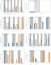 |
Fig. 10 Abundances for different molecule families (a–g) as described in Sect. 4. The blue and orange bars indicate the abundances of core and envelope components, respectively. The hatched bars indicate abundances in the hot core of Sgr B2(N) with respect to H2, derived by Neill et al. (2014). Since the distinction between ortho and para was not done by Neill et al. (2014), we compare theabundances of the ortho and para molecules with the unresolved results of Sgr B2(N). |
Ortho/para ratios for different molecules and velocity ranges.
6 Conclusions
We have presented a full HIFI chemical survey of the Sgr B2(M) star-forming region, which spans a frequency range from 480 to 1907 GHz. A total of 92 isotopologues arising from 49 molecules are detected in this survey through transitions in emission and absorption. Taking local overlap effects into account and assuming a two-layer model representing the core and the envelope of Sgr B2(M) with different dust concentrations, we performed LTE modeling using the XCLASS program, to the observed features of all molecules in the spectrum. About 14% of the data channels observed to have intensities over the 3σ level are currently unidentified. Sulfur dioxide is the strongest contributor to the HIFI survey both in terms of total integrated intensity and number of detected lines. Based on the obtained column densities, we computed molecular abundances for each detected species and compared them with those derived by Neill et al. (2014) for Sgr B2(N). For all but one molecular families we find bimodal distributions of the excitation temperatures with maxima around 20 and 500 K. For carbon, hydrocarbons, and for halogen molecules both maxima are shifted to lower temperatures. Furthermore, we derive ortho/para ratios for different molecules and velocity regions ranging from 1.2 to 4.6. Ratios above five and below one might be falsified by Non-LTE effects.
Acknowledgements
HIFI has been designed and built by a consortium of institutes and university departments from across Europe, Canada and the United States under the leadership of SRON Netherlands Institute for Space Research, Groningen, The Netherlands and with major contributions from Germany, France and the US. Consortium members are: Canada: CSA, U. Waterloo; France: CESR, LAB, LERMA, IRAM; Germany: KOSMA, MPIfR, MPS; Ireland, NUI Maynooth; Italy: ASI, IFSI-INAF, Osservatorio Astrofisico di Arcetri- INAF; Netherlands: SRON, TUD; Poland: CAMK, CBK; Spain: Observatorio Astronómico Nacional (IGN), Centro de Astrobiologìa (CSIC-INTA). Sweden: Chalmers University of Technology – MC2, RSS & GARD; Onsala Space Observatory; Swedish National Space Board, Stockholm University – Stockholm Observatory; Switzerland: ETH Zurich, FHNW; USA: Caltech, JPL, NHSC. Support for this work was provided by NASA through an award issued by JPL/Caltech. CSO is supported by the NSF, award AST-0540882. This work was supported by the Deutsche Forschungsgemeinschaft (DFG) through grant Collaborative Research Centre 956 (subproject A6 and C3, project ID 184018867) and from BMBF/Verbundforschung through the projects ALMA-ARC 05A14PK1 and ALMA-ARC 05A20PK1. Part of this research was carried out at the Jet Propulsion Laboratory, California Institute of Technology, under a contract with the National Aeronautics and Space Administration.
Appendix A LTE parameters
LTE Parameters for the Sgr B2(M) Full-band Model (Core Components).
LTE parameters for the Sgr B2(M) Full-band Model (Envelope Components).
Appendix B Plots
In each figure presented in this section the HIFI spectrum (blue line) is shown together with the overall fit (green dashed line) and the contribution of the respective molecule (red line), respectively. The vertical gray dashed line indicates the source velocity of Sgr B2(M).
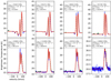 |
Fig. B.1 Selected transitions of CO (red line). |
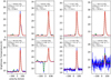 |
Fig. B.2 Selected transitions of 13CO (red line). |
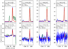 |
Fig. B.3 Selected transitions of C17O (red line). |
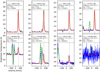 |
Fig. B.4 Selected transitions of C18O (red line). |
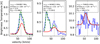 |
Fig. B.5 Selected transitions of 13C17O (red line). |
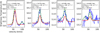 |
Fig. B.6 Selected transitions of 13C18O (red line). |
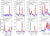 |
Fig. B.7 Selected transitions of CH3OH (red line). |
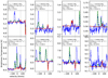 |
Fig. B.8 Selected transitions of 13CH3OH (red line). |
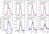 |
Fig. B.9 Selected transitions of ortho-H2CO (red line). |
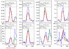 |
Fig. B.10 Selected transitions of para-H2CO (red line). |
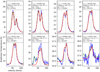 |
Fig. B.11 Selected transitions of HCO+ (red line). |
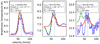 |
Fig. B.12 Selected transitions of H13CO+ (red line). |
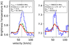 |
Fig. B.13 Selected transitions of HC18O+ (red line). |
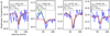 |
Fig. B.14 Selected transitions of HOCO+ (red line). |
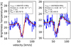 |
Fig. B.15 Selected transitions of OH (red line). |
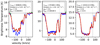 |
Fig. B.16 Selected transitions of OH+ (red line). |
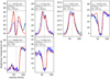 |
Fig. B.17 Selected transitions of ortho-H2O (red line). |
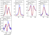 |
Fig. B.18 Selected transitions of para-H2O (red line). |
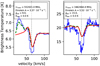 |
Fig. B.19 Selected transitions of ortho-H2 17O (red line). |
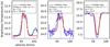 |
Fig. B.20 Selected transitions of para-H2 17O (red line). |
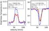 |
Fig. B.21 Selected transitions of ortho-H2 18O (red line). |
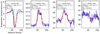 |
Fig. B.22 Selected transitions of para-H2 18O (red line). |
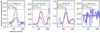 |
Fig. B.23 Selected transitions of HDO (red line). |
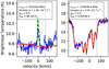 |
Fig. B.24 Selected transitions of ortho-H2O+ (red line). |
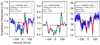 |
Fig. B.25 Selected transitions of para-H2O+ (red line). |
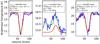 |
Fig. B.26 Selected transitions of ortho-H3O+ (red line). |
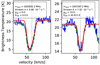 |
Fig. B.27 Selected transitions of para-H3O+ (red line). |
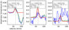 |
Fig. B.28 Selected transitions of SiO (red line). |
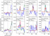 |
Fig. B.29 Selected transitions of CH3OCH3 (red line). |
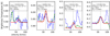 |
Fig. B.30 Selected transitions of CH3NH2 (red line). |
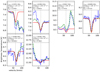 |
Fig. B.31 Selected transitions of CH2NH (red line). |
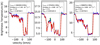 |
Fig. B.32 Selected transitions of NH (red line). |
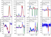 |
Fig. B.33 Selected transitions of ortho-NH2 (red line). |
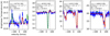 |
Fig. B.34 Selected transitions of para-NH2 (red line). |
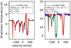 |
Fig. B.35 Selected transitions of ortho-NH3 (red line). |
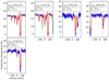 |
Fig. B.36 Selected transitions of para-NH3 (red line). |
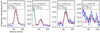 |
Fig. B.37 Selected transitions of N2H+ (red line). |
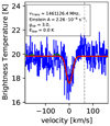 |
Fig. B.38 Selected transitions of 14N+ (red line). |
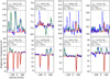 |
Fig. B.39 Selected transitions of HNCO (red line). |
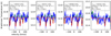 |
Fig. B.40 Selected transitions of HN13CO (red line). |
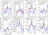 |
Fig. B.41 Selected transitions of NH2CHO (red line). |
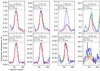 |
Fig. B.42 Selected transitions of NO (red line). |
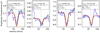 |
Fig. B.43 Selected transitions of HNO (red line). |
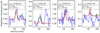 |
Fig. B.44 Selected transitions of N2O (red line). |
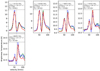 |
Fig. B.45 Selected transitions of HCN (red line). |
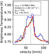 |
Fig. B.46 Selected transitions of H13CN (red line). |
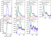 |
Fig. B.47 Selected transitions of HCN,v2 = 1 (red line). |
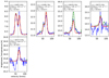 |
Fig. B.48 Selected transitions of HNC (red line). |
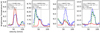 |
Fig. B.49 Selected transitions of HN13C (red line). |
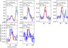 |
Fig. B.50 Selected transitions of HNC,v2 = 1 (red line). |
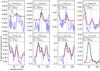 |
Fig. B.51 Selected transitions of CH3CN (red line). |
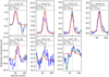 |
Fig. B.52 Selected transitions of CN (red line). |
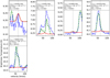 |
Fig. B.53 Selected transitions of 13CN (red line). |
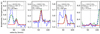 |
Fig. B.54 Selected transitions of HCCCN (red line). |
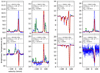 |
Fig. B.55 Selected transitions of ortho-H2S (red line). |
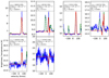 |
Fig. B.56 Selected transitions of para-H2S (red line). |
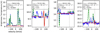 |
Fig. B.57 Selected transitions of ortho-H2 33S (red line). |
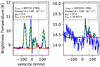 |
Fig. B.58 Selected transitions of para-H2 33S (red line). |
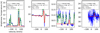 |
Fig. B.59 Selected transitions of ortho-H2 34S (red line). |
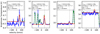 |
Fig. B.60 Selected transitions of para-H2 34S (red line). |
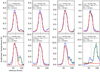 |
Fig. B.61 Selected transitions of SO (red line). |
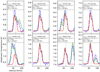 |
Fig. B.62 Selected transitions of 34SO (red line). |
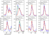 |
Fig. B.63 Selected transitions of SO2 (red line). |
 |
Fig. B.64 Selected transitions of 33SO2 (red line). |
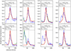 |
Fig. B.65 Selected transitions of 34SO2 (red line). |
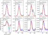 |
Fig. B.66 Selected transitions of CS (red line). |
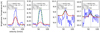 |
Fig. B.67 Selected transitions of 13CS (red line). |
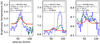 |
Fig. B.68 Selected transitions of C33S (red line). |
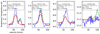 |
Fig. B.69 Selected transitions of C34S (red line). |
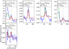 |
Fig. B.70 Selected transitions of H2CS (red line). |
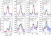 |
Fig. B.71 Selected transitions of OCS (red line). |
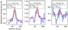 |
Fig. B.72 Selected transitions of HCS+ (red line). |
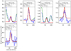 |
Fig. B.73 Selected transitions of NS (red line). |
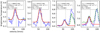 |
Fig. B.74 Selected transitions of SO+ (red line). |
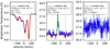 |
Fig. B.75 Selected transitions of SH+ (red line). |
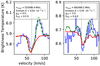 |
Fig. B.76 Selected transitions of 34SH+ (red line). |
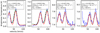 |
Fig. B.77 Selected transitions of CCH (red line). |
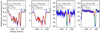 |
Fig. B.78 Selected transitions of CH (red line). |
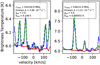 |
Fig. B.79 Selected transitions of 13CH (red line). |
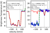 |
Fig. B.80 Selected transitions of CH+ (red line). |
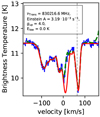 |
Fig. B.81 Selected transitions of 13CH+ (red line). |
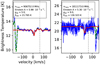 |
Fig. B.82 Selected transitions of CD+ (red line). |
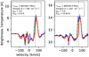 |
Fig. B.83 Selected transitions of 12C (red line). |
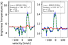 |
Fig. B.84 Selected transitions of 13C (red line). |
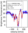 |
Fig. B.85 Selected transitions of 12C+ (red line). |
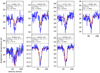 |
Fig. B.86 Selected transitions of C3 (red line). |
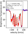 |
Fig. B.87 Selected transitions of HF (red line). |
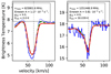 |
Fig. B.88 Selected transitions of HCl (red line). |
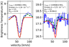 |
Fig. B.89 Selected transitions of H37Cl (red line). |
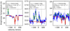 |
Fig. B.90 Selected transitions of ortho-H2Cl+ (red line). |
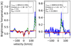 |
Fig. B.91 Selected transitions of para-H2Cl+ (red line). |
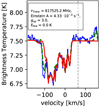 |
Fig. B.92 Selected transitions of 36ArH+ (red line). |
References
- Araki, M., Takano, S., Kuze, N., et al. 2020, MNRAS, 497, 1521 [CrossRef] [Google Scholar]
- Astropy Collaboration (Price-Whelan, A. M., et al.) 2018, AJ, 156, 123 [Google Scholar]
- Belloche, A., Müller, H. S. P., Menten, K. M., Schilke, P., & Comito, C. 2013, A&A, 559, A47 [NASA ADS] [CrossRef] [EDP Sciences] [Google Scholar]
- Bergin, E. A., Phillips, T. G., Comito, C., et al. 2010, A&A, 521, L20 [NASA ADS] [CrossRef] [EDP Sciences] [Google Scholar]
- Cernicharo, J., Goicoechea, J. R., & Caux, E. 2000, ApJ, 534, L199 [NASA ADS] [CrossRef] [PubMed] [Google Scholar]
- Cesaroni, R., & Walmsley, C. M. 1991, A&A, 241, 537 [NASA ADS] [Google Scholar]
- Churchwell, E., Wood, D., Myers, P. C., & Myers, R. V. 1986, ApJ, 305, 405 [NASA ADS] [CrossRef] [Google Scholar]
- Comito, C., Schilke, P., Rolffs, R., et al. 2010, A&A, 521, L38 [NASA ADS] [CrossRef] [EDP Sciences] [Google Scholar]
- Crockett, N. R., Bergin, E. A., Neill, J. L., et al. 2014, ApJ, 781, 114 [NASA ADS] [CrossRef] [Google Scholar]
- Cummins, S. E., Linke, R. A., & Thaddeus, P. 1986, ApJS, 60, 819 [NASA ADS] [CrossRef] [Google Scholar]
- de Graauw, T., Helmich, F. P., Phillips, T. G., et al. 2010, A&A, 518, L6 [NASA ADS] [CrossRef] [EDP Sciences] [Google Scholar]
- de Vicente, P., Martin-Pintado, J., & Wilson, T. L. 1997, A&A, 320, 957 [NASA ADS] [Google Scholar]
- Dickens, J. E., & Irvine, W. M. 1999, ApJ, 518, 733 [NASA ADS] [CrossRef] [Google Scholar]
- Endres, C. P., Schlemmer, S., Schilke, P., Stutzki, J., & Müller, H. S. P. 2016, J. Mol. Spectr., 327, 95 [NASA ADS] [CrossRef] [Google Scholar]
- Etxaluze, M., Goicoechea, J. R., Cernicharo, J., et al. 2013, A&A, 556, A137 [NASA ADS] [CrossRef] [EDP Sciences] [Google Scholar]
- Faure, A., Hily-Blant, P., Le Gal, R., Rist, C., & Pineau des Forêts, G. 2013, ApJ, 770, L2 [NASA ADS] [CrossRef] [Google Scholar]
- Faure, A., Hily-Blant, P., Rist, C., et al. 2019, MNRAS, 487, 3392 [CrossRef] [Google Scholar]
- Foreman-Mackey, D. 2016, J. Open Source Softw., 1, 24 [Google Scholar]
- Foreman-Mackey, D., Hogg, D. W., Lang, D., & Goodman, J. 2013, PASP, 125, 306 [Google Scholar]
- Friedel, D. N., Snyder, L. E., Turner, B. E., & Remijan, A. 2004, ApJ, 600, 234 [NASA ADS] [CrossRef] [Google Scholar]
- Friesen, R. K., Di Francesco, J., Bourke, T. L., et al. 2014, ApJ, 797, 27 [NASA ADS] [CrossRef] [Google Scholar]
- Fuchs, G. W., Fuchs, U., Giesen, T. F., & Wyrowski, F. 2005, A&A, 444, 521 [NASA ADS] [CrossRef] [EDP Sciences] [Google Scholar]
- Fuchs, G. W., Cuppen, H. M., Ioppolo, S., et al. 2009, A&A, 505, 629 [NASA ADS] [CrossRef] [EDP Sciences] [Google Scholar]
- Garrod, R. T. 2013, ApJ, 778, 158 [NASA ADS] [CrossRef] [Google Scholar]
- Garrod, R. T., & Pauly, T. 2011, ApJ, 735, 15 [NASA ADS] [CrossRef] [Google Scholar]
- Gerin, M., de Luca, M., Lis, D. C., et al. 2013, J. Phys. Chem. A, 117, 10018 [CrossRef] [Google Scholar]
- Giesen, T. F., Mookerjea, B., Fuchs, G. W., et al. 2020, A&A, 633, A120 [CrossRef] [EDP Sciences] [Google Scholar]
- Godard, B., Falgarone, E., Gerin, M., et al. 2012, A&A, 540, A87 [NASA ADS] [CrossRef] [EDP Sciences] [Google Scholar]
- Goicoechea, J. R., & Cernicharo, J. 2002, ApJ, 576, L77 [NASA ADS] [CrossRef] [Google Scholar]
- Goicoechea, J. R., Cernicharo, J., & Caux, E. 2000, ESA SP, 456, 99 [Google Scholar]
- Goldsmith, P. F., Snell, R. L., & Lis, D. C. 1987, ApJ, 313, L5 [NASA ADS] [CrossRef] [Google Scholar]
- Goldsmith, P. F., Lis, D. C., Lester, D. F., & Harvey, P. M. 1992, ApJ, 389, 338 [NASA ADS] [CrossRef] [Google Scholar]
- Goodman, J., & Weare, J. 2010, Commun. Appl. Math. Comput. Sci., 5, 65 [Google Scholar]
- GRAVITY Collaboration (Abuter, R., et al.) 2019, A&A, 625, L10 [NASA ADS] [CrossRef] [EDP Sciences] [Google Scholar]
- Greaves, J. S., & Williams, P. G. 1994, A&A, 290, 259 [NASA ADS] [Google Scholar]
- Hildebrand, R. H. 1983, QJRAS, 24, 267 [NASA ADS] [Google Scholar]
- Hüttemeister, S., Wilson, T. L., Mauersberger, R., et al. 1995, A&A, 294, 667 [NASA ADS] [Google Scholar]
- Le Gal, R., Herbst, E., Xie, C., Li, A., & Guo, H. 2016, A&A, 596, A35 [NASA ADS] [CrossRef] [EDP Sciences] [Google Scholar]
- Lis, D. C., & Goldsmith, P. F. 1989, ApJ, 337, 704 [NASA ADS] [CrossRef] [Google Scholar]
- Lis, D. C., Phillips, T. G., Goldsmith, P. F., et al. 2010, A&A, 521, L26 [NASA ADS] [CrossRef] [EDP Sciences] [Google Scholar]
- Lis, D. C., Schilke, P., Bergin, E. A., et al. 2014, ApJ, 785, 135 [NASA ADS] [CrossRef] [Google Scholar]
- Mangum, J. G., & Shirley, Y. L. 2015, PASP, 127, 266 [Google Scholar]
- Meng, F., Sánchez-Monge, Á., Schilke, P., et al. 2019, A&A, 630, A73 [NASA ADS] [CrossRef] [EDP Sciences] [Google Scholar]
- Menten, K. M., Wyrowski, F., Belloche, A., et al. 2011, A&A, 525, A77 [NASA ADS] [CrossRef] [EDP Sciences] [Google Scholar]
- Möller, T., Endres, C., & Schilke, P. 2017, A&A, 598, A7 [NASA ADS] [CrossRef] [EDP Sciences] [Google Scholar]
- Monje, R. R., Emprechtinger, M., Phillips, T. G., et al. 2011, ApJ, 734, L23 [NASA ADS] [CrossRef] [Google Scholar]
- Müller, H. S. P., Thorwirth, S., Roth, D. A., & Winnewisser, G. 2001, A&A, 370, L49 [NASA ADS] [CrossRef] [EDP Sciences] [Google Scholar]
- Müller, H. S. P., Schlöder, F., Stutzki, J., & Winnewisser, G. 2005, J. Mol. Struc., 742, 215 [Google Scholar]
- Neill, J. L., Bergin, E. A., Lis, D. C., et al. 2014, ApJ, 789, 8 [NASA ADS] [CrossRef] [Google Scholar]
- Nummelin, A., Bergman, P., Hjalmarson, Å., et al. 1998, ApJS, 117, 427 [NASA ADS] [CrossRef] [Google Scholar]
- Ossenkopf, V.,& Henning, T. 1994, A&A, 291, 943 [Google Scholar]
- Parzen, E. 1962, Ann. Math. Stat., 33, 1065 [NASA ADS] [CrossRef] [MathSciNet] [Google Scholar]
- Pickett, H. M., Poynter, R. L., Cohen, E. A., et al. 1998, J. Quant. Spectr. Rad. Transf., 60, 883 [Google Scholar]
- Pilbratt, G. L., Riedinger, J. R., Passvogel, T., et al. 2010, A&A, 518, L1 [CrossRef] [EDP Sciences] [Google Scholar]
- Polehampton, E. T., Baluteau, J.-P., Swinyard, B. M., et al. 2007, MNRAS, 377, 1122 [Google Scholar]
- Putaud, T., Michaut, X., Le Petit, F., Roueff, E., & Lis, D. C. 2019, A&A, 632, A8 [NASA ADS] [CrossRef] [EDP Sciences] [Google Scholar]
- Qin, S. L., Schilke, P., Comito, C., et al. 2010, A&A, 521, L14 [NASA ADS] [CrossRef] [EDP Sciences] [Google Scholar]
- Qin, S. L., Schilke, P., Rolffs, R., et al. 2011, A&A, 530, L9 [NASA ADS] [CrossRef] [EDP Sciences] [Google Scholar]
- Roelfsema, P. R., Helmich, F. P., Teyssier, D., et al. 2012, A&A, 537, A17 [NASA ADS] [CrossRef] [EDP Sciences] [Google Scholar]
- Rolffs, R., Schilke, P., Comito, C., et al. 2010, A&A, 521, L46 [NASA ADS] [CrossRef] [EDP Sciences] [Google Scholar]
- Rosenblatt, M. 1956, Ann. Math. Stat., 27, 832 [CrossRef] [MathSciNet] [Google Scholar]
- Sánchez-Monge, Á., Schilke, P., Schmiedeke, A., et al. 2017, A&A, 604, A6 [NASA ADS] [CrossRef] [EDP Sciences] [Google Scholar]
- Schilke, P., Comito, C., Müller, H. S. P., et al. 2010, A&A, 521, L11 [CrossRef] [EDP Sciences] [Google Scholar]
- Schilke, P., Neufeld, D. A., Müller, H. S. P., et al. 2014, A&A, 566, A29 [NASA ADS] [CrossRef] [EDP Sciences] [Google Scholar]
- Schmiedeke, A., Schilke, P., Möller, T., et al. 2016, A&A, 588, A143 [NASA ADS] [CrossRef] [EDP Sciences] [Google Scholar]
- Schwörer, A., Sánchez-Monge, Á., Schilke, P., et al. 2019, A&A, 628, A6 [NASA ADS] [CrossRef] [EDP Sciences] [Google Scholar]
- Silverman, B. W. 1986, Density Estimation for Statistics and Data Analysis (Boca Raton: Taylor and Francis) [Google Scholar]
- Sofue, Y. 2006, PASJ, 58, 335 [NASA ADS] [Google Scholar]
- Sutton, E. C., Jaminet, P. A., Danchi, W. C., & Blake, G. A. 1991, ApJS, 77, 255 [NASA ADS] [CrossRef] [Google Scholar]
- Tieftrunk, A., Pineau des Forets, G., Schilke, P., & Walmsley, C. M. 1994, A&A, 289, 579 [Google Scholar]
- Turner, B. E. 1989, ApJS, 70, 539 [NASA ADS] [CrossRef] [Google Scholar]
- Turner, B. E. 1991, ApJS, 76, 617 [NASA ADS] [CrossRef] [Google Scholar]
- Vallée, J. P. 2008, AJ, 135, 1301 [NASA ADS] [CrossRef] [Google Scholar]
- Virtanen, P., Gommers, R., Oliphant, T. E., et al. 2020, Nat. Methods, 17, 261 [Google Scholar]
- Whiteoak, J. B., & Gardner, F. F. 1979, MNRAS, 188, 445 [NASA ADS] [Google Scholar]
- Winnewisser, G., & Gardner, F. F. 1976, A&A, 48, 159 [Google Scholar]
- Xu, L.-H., Fisher, J., Lees, R. M., et al. 2008, J. Mol. Spectr., 251, 305 [NASA ADS] [CrossRef] [Google Scholar]
- Zmuidzinas, J., Blake, G. A., Carlstrom, J., Keene, J., & Miller, D. 1995, ApJ, 447, L125 [NASA ADS] [CrossRef] [PubMed] [Google Scholar]
In order to be consistent with previous models we use a distance of 8.5 kpc in the rest of the paper.
The fitted spectra are published at the CDS.
As a kind of continuous replacement of a discrete histogram the KDE is a function
 applied to a distribution xi
of n
points
applied to a distribution xi
of n
points
![Mathematical equation: $\displaystyle {\widehat {f}}_{h}(x) = \frac{1}{n \, h} \sum _{i = 1}^{n} K \Big[ \frac{x - x_{i}}{h} \Big], \hfill (6) $](/articles/aa/full_html/2021/07/aa40203-20/aa40203-20-eq77.png) (6) where K(x) is called the kernel function that is mostly a Gaussian and h > 0 indicates the bandwidth that controls the amount of smoothing. Here, Silverman’s rule (Silverman 1986) as scipy implementation (Virtanen et al. 2020) is used to compute the bandwidth h
of each KDE.
(6) where K(x) is called the kernel function that is mostly a Gaussian and h > 0 indicates the bandwidth that controls the amount of smoothing. Here, Silverman’s rule (Silverman 1986) as scipy implementation (Virtanen et al. 2020) is used to compute the bandwidth h
of each KDE.
All Tables
Velocity ranges corresponding to different kinematic components, taken from Lis et al. (2014).
Integrated line intensities for each molecule in the model to the Sgr B2(M) spectral survey.
All Figures
|
Fig. 1 ALMA 235.5 GHz continuum image of Sgr B2(M) at 0.4′′ angular resolution (Sánchez-Monge et al. 2017, from) with the FWHM HIFI beam at 480 (band 1a) and 1907 GHz (band 7b) shown as red and green circles, respectively. |
| In the text | |
|
Fig. 2 Full view of the (uncorrected) Sgr B2(M) HIFI survey, where the HIFI bands are divided into “a” (blue) and “b” (black) bands) |
| In the text | |
|
Fig. 3 Spectrum of the 1 837 816.8 MHz transition of OH. The full LTE model of OH (green dashed line) is superposed on the HIFIspectrum (black histogram). The contribution of the core and the envelope are shown as blue and orange lines, respectively. In order to determine the integrated intensities of different components and velocity ranges we take only those components into account, which belong to a specific range. By doing so we neglect the contributions from other components as shown here. The sum of integrated intensities of core and envelope contributions is about a factor two higher than the integrated intensity of the full LTE model. |
| In the text | |
|
Fig. 4 Example of unidentified peaks in the HIFI survey of Sgr B2(M) in band 1b. The observed spectrum is shown in black, the full model in red, and the cyan dashed line marks the continuum level. The blue area represents the + ∕−3σ level, i.e., all peaks that do not protrude from this area are ignored. The height and width of the unidentified feature near 620.7 GHZ is described by the horizontal and vertical green line, respectively. The peaks indicated by the small gray vertical lines are ignored, because their line widths are below the lower limit of the allowed range of line widths. |
| In the text | |
|
Fig. 5 Fraction of unidentified peaks as function of band. |
| In the text | |
|
Fig. 6 Ten strongest cooling molecules in Sgr B2(M) in the frequency ranges covered with HIFI. |
| In the text | |
|
Fig. 7 Excerpts of the HIFI survey of Sgr B2(M) in bands 1a and 3b (solid black line), with the full model (dashed green line) and those of the molecules contributing to the spectral range of each panel. |
| In the text | |
|
Fig. 8 Corner plot (Foreman-Mackey 2016) showing the one and two dimensional projections of the posterior probability distributions of the model parameters of CN. On top of each column the probability distribution for each free parameter is shown together with the value of the best fit and the corresponding left and right errors. The left and right dashed lines indicate the lower and upper limits of the corresponding HPD interval, respectively. The dashed line in the middle indicates the mode of the distribution. The blue lines indicate the parameter values of the best fit. The plots in the lower left corner describe the projected 2D histograms of two parameters and the contours the HPD regions, respectively. In order to get a better estimation of the errors, we determine the error of the column density on log scale and use the velocity offset (voff) related to the source velocity of vLSR = 64 km s−1. |
| In the text | |
|
Fig. 9 Normalized KDE for different model parameters and molecule families defined in Sect. 4. Additionally, the bandwidth h of all KDEs used for each molecule family is given as well. The gray areas in d indicate the velocity ranges described in Table 1. The families “complex O-bearing molecules” (Sect. 4.2) and “other molecules” (Sect. 4.9) are not shown, because they contain only one molecule, respectively. |
| In the text | |
|
Fig. 10 Abundances for different molecule families (a–g) as described in Sect. 4. The blue and orange bars indicate the abundances of core and envelope components, respectively. The hatched bars indicate abundances in the hot core of Sgr B2(N) with respect to H2, derived by Neill et al. (2014). Since the distinction between ortho and para was not done by Neill et al. (2014), we compare theabundances of the ortho and para molecules with the unresolved results of Sgr B2(N). |
| In the text | |
|
Fig. B.1 Selected transitions of CO (red line). |
| In the text | |
|
Fig. B.2 Selected transitions of 13CO (red line). |
| In the text | |
|
Fig. B.3 Selected transitions of C17O (red line). |
| In the text | |
|
Fig. B.4 Selected transitions of C18O (red line). |
| In the text | |
|
Fig. B.5 Selected transitions of 13C17O (red line). |
| In the text | |
|
Fig. B.6 Selected transitions of 13C18O (red line). |
| In the text | |
|
Fig. B.7 Selected transitions of CH3OH (red line). |
| In the text | |
|
Fig. B.8 Selected transitions of 13CH3OH (red line). |
| In the text | |
|
Fig. B.9 Selected transitions of ortho-H2CO (red line). |
| In the text | |
|
Fig. B.10 Selected transitions of para-H2CO (red line). |
| In the text | |
|
Fig. B.11 Selected transitions of HCO+ (red line). |
| In the text | |
|
Fig. B.12 Selected transitions of H13CO+ (red line). |
| In the text | |
|
Fig. B.13 Selected transitions of HC18O+ (red line). |
| In the text | |
|
Fig. B.14 Selected transitions of HOCO+ (red line). |
| In the text | |
|
Fig. B.15 Selected transitions of OH (red line). |
| In the text | |
|
Fig. B.16 Selected transitions of OH+ (red line). |
| In the text | |
|
Fig. B.17 Selected transitions of ortho-H2O (red line). |
| In the text | |
|
Fig. B.18 Selected transitions of para-H2O (red line). |
| In the text | |
|
Fig. B.19 Selected transitions of ortho-H2 17O (red line). |
| In the text | |
|
Fig. B.20 Selected transitions of para-H2 17O (red line). |
| In the text | |
|
Fig. B.21 Selected transitions of ortho-H2 18O (red line). |
| In the text | |
|
Fig. B.22 Selected transitions of para-H2 18O (red line). |
| In the text | |
|
Fig. B.23 Selected transitions of HDO (red line). |
| In the text | |
|
Fig. B.24 Selected transitions of ortho-H2O+ (red line). |
| In the text | |
|
Fig. B.25 Selected transitions of para-H2O+ (red line). |
| In the text | |
|
Fig. B.26 Selected transitions of ortho-H3O+ (red line). |
| In the text | |
|
Fig. B.27 Selected transitions of para-H3O+ (red line). |
| In the text | |
|
Fig. B.28 Selected transitions of SiO (red line). |
| In the text | |
|
Fig. B.29 Selected transitions of CH3OCH3 (red line). |
| In the text | |
|
Fig. B.30 Selected transitions of CH3NH2 (red line). |
| In the text | |
|
Fig. B.31 Selected transitions of CH2NH (red line). |
| In the text | |
|
Fig. B.32 Selected transitions of NH (red line). |
| In the text | |
|
Fig. B.33 Selected transitions of ortho-NH2 (red line). |
| In the text | |
|
Fig. B.34 Selected transitions of para-NH2 (red line). |
| In the text | |
|
Fig. B.35 Selected transitions of ortho-NH3 (red line). |
| In the text | |
|
Fig. B.36 Selected transitions of para-NH3 (red line). |
| In the text | |
|
Fig. B.37 Selected transitions of N2H+ (red line). |
| In the text | |
|
Fig. B.38 Selected transitions of 14N+ (red line). |
| In the text | |
|
Fig. B.39 Selected transitions of HNCO (red line). |
| In the text | |
|
Fig. B.40 Selected transitions of HN13CO (red line). |
| In the text | |
|
Fig. B.41 Selected transitions of NH2CHO (red line). |
| In the text | |
|
Fig. B.42 Selected transitions of NO (red line). |
| In the text | |
|
Fig. B.43 Selected transitions of HNO (red line). |
| In the text | |
|
Fig. B.44 Selected transitions of N2O (red line). |
| In the text | |
|
Fig. B.45 Selected transitions of HCN (red line). |
| In the text | |
|
Fig. B.46 Selected transitions of H13CN (red line). |
| In the text | |
|
Fig. B.47 Selected transitions of HCN,v2 = 1 (red line). |
| In the text | |
|
Fig. B.48 Selected transitions of HNC (red line). |
| In the text | |
|
Fig. B.49 Selected transitions of HN13C (red line). |
| In the text | |
|
Fig. B.50 Selected transitions of HNC,v2 = 1 (red line). |
| In the text | |
|
Fig. B.51 Selected transitions of CH3CN (red line). |
| In the text | |
|
Fig. B.52 Selected transitions of CN (red line). |
| In the text | |
|
Fig. B.53 Selected transitions of 13CN (red line). |
| In the text | |
|
Fig. B.54 Selected transitions of HCCCN (red line). |
| In the text | |
|
Fig. B.55 Selected transitions of ortho-H2S (red line). |
| In the text | |
|
Fig. B.56 Selected transitions of para-H2S (red line). |
| In the text | |
|
Fig. B.57 Selected transitions of ortho-H2 33S (red line). |
| In the text | |
|
Fig. B.58 Selected transitions of para-H2 33S (red line). |
| In the text | |
|
Fig. B.59 Selected transitions of ortho-H2 34S (red line). |
| In the text | |
|
Fig. B.60 Selected transitions of para-H2 34S (red line). |
| In the text | |
|
Fig. B.61 Selected transitions of SO (red line). |
| In the text | |
|
Fig. B.62 Selected transitions of 34SO (red line). |
| In the text | |
|
Fig. B.63 Selected transitions of SO2 (red line). |
| In the text | |
|
Fig. B.64 Selected transitions of 33SO2 (red line). |
| In the text | |
|
Fig. B.65 Selected transitions of 34SO2 (red line). |
| In the text | |
|
Fig. B.66 Selected transitions of CS (red line). |
| In the text | |
|
Fig. B.67 Selected transitions of 13CS (red line). |
| In the text | |
|
Fig. B.68 Selected transitions of C33S (red line). |
| In the text | |
|
Fig. B.69 Selected transitions of C34S (red line). |
| In the text | |
|
Fig. B.70 Selected transitions of H2CS (red line). |
| In the text | |
|
Fig. B.71 Selected transitions of OCS (red line). |
| In the text | |
|
Fig. B.72 Selected transitions of HCS+ (red line). |
| In the text | |
|
Fig. B.73 Selected transitions of NS (red line). |
| In the text | |
|
Fig. B.74 Selected transitions of SO+ (red line). |
| In the text | |
|
Fig. B.75 Selected transitions of SH+ (red line). |
| In the text | |
|
Fig. B.76 Selected transitions of 34SH+ (red line). |
| In the text | |
|
Fig. B.77 Selected transitions of CCH (red line). |
| In the text | |
|
Fig. B.78 Selected transitions of CH (red line). |
| In the text | |
|
Fig. B.79 Selected transitions of 13CH (red line). |
| In the text | |
|
Fig. B.80 Selected transitions of CH+ (red line). |
| In the text | |
|
Fig. B.81 Selected transitions of 13CH+ (red line). |
| In the text | |
|
Fig. B.82 Selected transitions of CD+ (red line). |
| In the text | |
|
Fig. B.83 Selected transitions of 12C (red line). |
| In the text | |
|
Fig. B.84 Selected transitions of 13C (red line). |
| In the text | |
|
Fig. B.85 Selected transitions of 12C+ (red line). |
| In the text | |
|
Fig. B.86 Selected transitions of C3 (red line). |
| In the text | |
|
Fig. B.87 Selected transitions of HF (red line). |
| In the text | |
|
Fig. B.88 Selected transitions of HCl (red line). |
| In the text | |
|
Fig. B.89 Selected transitions of H37Cl (red line). |
| In the text | |
|
Fig. B.90 Selected transitions of ortho-H2Cl+ (red line). |
| In the text | |
|
Fig. B.91 Selected transitions of para-H2Cl+ (red line). |
| In the text | |
|
Fig. B.92 Selected transitions of 36ArH+ (red line). |
| In the text | |
Current usage metrics show cumulative count of Article Views (full-text article views including HTML views, PDF and ePub downloads, according to the available data) and Abstracts Views on Vision4Press platform.
Data correspond to usage on the plateform after 2015. The current usage metrics is available 48-96 hours after online publication and is updated daily on week days.
Initial download of the metrics may take a while.