| Issue |
A&A
Volume 651, July 2021
|
|
|---|---|---|
| Article Number | A65 | |
| Number of page(s) | 18 | |
| Section | Numerical methods and codes | |
| DOI | https://doi.org/10.1051/0004-6361/202040152 | |
| Published online | 14 July 2021 | |
SRoll3: A neural network approach to reduce large-scale systematic effects in the Planck High-Frequency Instrument maps
1
Université Paris-Saclay, CNRS, Institut d’Astrophysique Spatiale, 91405 Orsay, France
e-mail: This email address is being protected from spambots. You need JavaScript enabled to view it.
2
Laboratoire d’Océanographie Physique et Spatiale, CNRS, 29238 Plouzané, France
Received:
17
December
2020
Accepted:
27
April
2021
Abstract
In the present work, we propose a neural-network-based data-inversion approach to reduce structured contamination sources, with a particular focus on the mapmaking for Planck High Frequency Instrument data and the removal of large-scale systematic effects within the produced sky maps. The removal of contamination sources is made possible by the structured nature of these sources, which is characterized by local spatiotemporal interactions producing couplings between different spatiotemporal scales. We focus on exploring neural networks as a means of exploiting these couplings to learn optimal low-dimensional representations, which are optimized with respect to the contamination-source-removal and mapmaking objectives, to achieve robust and effective data inversion. We develop multiple variants of the proposed approach, and consider the inclusion of physics-informed constraints and transfer-learning techniques. Additionally, we focus on exploiting data-augmentation techniques to integrate expert knowledge into an otherwise unsupervised network-training approach. We validate the proposed method on Planck High Frequency Instrument 545 GHz Far Side Lobe simulation data, considering ideal and nonideal cases involving partial, gap-filled, and inconsistent datasets, and demonstrate the potential of the neural-network-based dimensionality reduction to accurately model and remove large-scale systematic effects. We also present an application to real Planck High Frequency Instrument 857 GHz data, which illustrates the relevance of the proposed method to accurately model and capture structured contamination sources, with reported gains of up to one order of magnitude in terms of performance in contamination removal. Importantly, the methods developed in this work are to be integrated in a new version of the SRoll algorithm (SRoll3), and here we describe SRoll3 857 GHz detector maps that were released to the community.
Key words: cosmology: observations / methods: data analysis / surveys / techniques: image processing
© M. Lopez-Radcenco et al. 2021
 Open Access article, published by EDP Sciences, under the terms of the Creative Commons Attribution License (https://creativecommons.org/licenses/by/4.0), which permits unrestricted use, distribution, and reproduction in any medium, provided the original work is properly cited.
1. Introduction
In the last few decades, scientific instruments have been producing ever increasing quantities of data. Moreover, as remote sensing and instrumentation technology develops, the processing complexity of the produced datasets increases dramatically. The ambitious objectives of several scientific projects are characterized by the reconstruction of the information present in these datasets, which is often mixed with additional contamination sources, such as systematic effects and foreground signals (physical components of the data that mask or blur part of the signal of interest). The scientific community is confronted, in a wide variety of contexts, with the need to extract, from measurements, physical responses adapted to the different models considered, while at the same time ensuring an effective separation between these responses and different contamination sources. This separation is made possible by two main factors. On one hand, the separation is achieved by exploiting the structured nature (in a stochastic sense) of the contamination sources, which, from a mathematical point of view, is characterized by local spatiotemporal interactions producing couplings between different spatiotemporal scales, as opposed to Gaussian signals where no correlation exists between observations produced at different spatiotemporal locations. The structured nature of such signals allows them to be accurately represented using a reduced number of degrees of freedom, which we aim to exploit in order to separate them from the signal of interest. On the other hand, the separation is possible thanks to the existence of spatial or temporal invariances and/or redundancy in the signal of interest, which can be used to partially remove the signal of interest from observations, as opposed to other structured but variable contamination sources that cannot be easily removed from data. It is important to notice that these two criteria are complementary, and serve different but equally important purposes. While the invariances within the signal of interest allows us to remove it from observations, and thus focus solely on adequately modeling the remaining contamination sources, such modeling is only made possible by the structured nature of these sources, which can be adequately represented using a reduced number of degrees of freedom. This interdependence between multiple criteria within the signal of interest and the contamination sources naturally favors the use of approaches that are designed to invert the data and remove the contamination sources simultaneously. Given that the aforementioned problem exists in multiple scientific contexts, developing efficient dimensionality reduction methods to accurately extract relevant information from data appears to be a key issue for the scientific community. It is therefore essential to identify representations involving a reduced number of degrees of freedom to achieve robust and effective data inversion, while providing enhanced capabilities to accurately describe the complexity of the processes and variabilities at play. In this regard, different strategies can be envisaged, with recent advances relying most notably on the exploitation of operators learned from data presenting some similarities with the problem of interest (e.g., transfer learning, as explained below). Alternatively, recent works explore the use of generic signal decomposition operators (e.g., scattering transforms Bruna et al. 2015). Efforts of this type have already yielded interesting results; for example, on the expected statistical description of galactic dust emissions (Allys et al. 2019).
In the present work, we specifically consider a case study involving the processing of Planck High Frequency Instrument (Planck-HFI) data, with a particular focus on the separation and removal of the large-scale systematic effects. In this context, we aim to exploit machine learning and artificial intelligence approaches to minimize the number of degrees of freedom of the large-scale systematic effects to be reconstructed and separated, whereas previous works rely on exploiting spectral and bispectral representations (Prunet et al. 2001; Doré et al. 2001; Natoli et al. 2001; Maino et al. 2002; de Gasperis et al. 2005; Keihänen et al. 2005, 2010; Poutanen et al. 2006; Armitage-Caplan & Wandelt 2009; Planck Collaboration VIII 2014; Delouis et al. 2019), which lack the ability to properly capture spatiotemporal scale interactions needed to tackle this issue. Indeed, large-scale systematic effects are usually represented using a large number of parameters, whereas more appropriate low-dimensional representations could be learned directly from data. Particularly, in the present work, we focus on exploring neural networks as a means of learning, from data, optimal low-dimensional representations that allow for the effective separation of the structured systematic effects from the signal of interest simultaneously with the data inversion. The algorithmic originality of this work lies in the integration of analysis methods issued from machine learning and artificial intelligence to extract the signals of interest from data by minimizing the degrees of freedom of the processes to be reconstructed within a classic minimization framework. As such, the objective of the proposed methods is to find the best low-dimensional description of the data while ensuring an optimal separation of the signal of interest from any systematic effects. We illustrate the relevance of our approach on a case study involving contamination-source removal and mapmaking, that is, the inversion of raw satellite measurements to produce a physically consistent spatial map of Planck-HFI data. We consider both Far Side Lobe pickup (FSL) (an unwanted signal due to the nonideal response of the satellite antenna) simulations from the 545 GHz Planck-HFI channel and real observations from the 857 GHz Planck-HFI channel. This case study was chosen based on the fact that the FSL pickup is a large-scale systematic effect that currently remains difficult to model and remove, given that the complexity of the Planck optical system forces current FSL estimations to rely on simplified physical and mathematical models. Specifically, current FSL models used to fit and remove FSL pickup rely on numerical simulations exploiting the GRASP tool (Tauber et al. 2010b), and considering mono-modal feedhorn models, whereas the Planck-HFI 545 GHz and 857 GHz channels use specialized multimode feedhorns. Modeling these feedhorns would require more complex, physically relevant models better suited to accurately depicting the FSL signal, but such highly complex models are not analytically or numerically feasible. In particular, Planck-HFI 545 GHz and 857 GHz channels present a weak cosmic microwave background (CMB) signature and its sources of contamination are dominated by the FSL pickup, which makes them ideal candidates for the considered case study. Importantly, this work builds on previously developed methods for the separation and removal of structured contamination sources –particularly on the SRoll2 algorithm (Delouis et al. 2019)– used for the production of the 2018 release of the Planck-HFI sky maps. As such, the methods developed in this work are to be integrated in a new version of the SRoll algorithm (SRoll3), and we describe here SRoll3 857 GHz detector maps that were released to the community. Finally, whereas the application presented provides strong evidence of the relevance of the proposed approach for the processing of large-scale systematic effects, the proposed methodology provides a generic framework for addressing similar, yet complex, data inversion issues involving the separation and removal of structured noise, foregrounds, and systematic effects from data in many other scientific domains.
Artificial neural networks are a class of machine learning algorithms that are designed to identify underlying relationships in data. Generally speaking, a neural network relies on a cascade of interconnected units or neurons. Each unit is capable of simple nonlinear processing of data. To this end, a neuron performs an affine transformation of a multidimensional input using a set of weights and biases, and subsequently exploits a nonlinear activation function to produce a scalar output. Neurons can then be stacked in parallel to produce multidimensional outputs. Moreover, by cascading multiple groups of parallelized neurons together, a deep neural network is capable of combining these simple processing units to model and learn highly complex nonlinear relationships directly from data. A schematic representation of this principle is included in Fig. 1. Building on this idea, the convolutional neural network (CNN) (LeCun et al. 1998), which considers neurons that only take into account a local sub-ensemble of the total inputs of the layer, was later introduced. In this way, adjacent neurons at each layer will take into account overlapping sub-ensembles of the inputs of the layer in a sliding window manner. Inputs considered by each neuron are thus partially shared locally. Mathematically, this can be seen as a convolution operator, where the output of the layer can be obtained by the convolution of the input with a convolution kernel comprised of the layer weights, followed by the addition of a set of biases. Typically, a nonlinear activation function, usually a regularized linear unit (ReLU), that is, ReLU(x) = max(0, x), is introduced to allow for nonlinear behavior. Dimensionality reduction or expansion is then achieved by a pooling operator, typically a local averaging or a local maxima. By feeding the output of one layer as input to another layer, multiple layers are then stacked in cascade to build a larger CNN model. Network training then consists in learning, from a training dataset, the network weights and biases that minimize a specific cost function, which is chosen based on the problem of interest. Here, we focus on using CNNs for extracting relevant information by finding low-dimensional representations of data. To this end, CNNs exploit the existence of invariances within the considered datasets (LeCun et al. 1998).
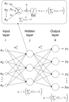 |
Fig. 1. Artificial neural network. An ensemble of simple processing units or neurons are connected in parallel and cascaded to produce a neural network capable of modeling highly complex, nonlinear, multidimensional relationships. For each neuron, output y is produced by an affine transformation of inputs xi by means of weights wi and bias b, followed by the application of a nonlinear activation function f. |
Autoencoder networks (Bourlard & Kamp 1988; Hinton & Salakhutdinov 2006) are the most commonly used neural network for producing low-dimensional representations of data. They rely on a symmetric architecture comprised of mirrored encoder and decoder networks, with a dimension bottleneck at the middle layer. As such, the decoder network processes inputs to produce a low-dimensional representation at the middle layer. This representation is processed by the decoder network to rebuild the original input as closely as possible. In this work, rather than using a classical autoencoder network, we focus exclusively on the decoder half of the autoencoder, and exploit input-training (Tan & Mayrovouniotis 1995; Hassoun & Sudjianto 1997) to train a deconvolutional decoder network directly from data. In this way, both the decoder network parameters as well as the optimal low-dimensional representation of the considered dataset (which constitutes the input of the decoder network) are learned simultaneously during the data inversion, without any preliminary network-training phase. The idea of a joint optimization of network parameters and inputs, known as input training, was first introduced by Tan & Mayrovouniotis (1995) and later revisited by Hassoun & Sudjianto (1997) in the context of autoencoder training. Input training, which closely relates to nonlinear principal component analysis (Baldi & Hornik 1989; Kramer 1991; Schölkopf et al. 1998; Scholz 2002; Scholz et al. 2005), was subsequently exploited for multiple applications, including error and fault detection and diagnosis (Reddy et al. 1996; Reddy & Mavrovouniotis 1998; Jia et al. 1998; Böhme et al. 1999; Erguo & Jinshou 2002; Bouakkaz & Harkat 2012), chemical process control, monitoring and modeling (Böhme et al. 1999; Liu & Zhao 2004; Geng & Zhu 2005; Zhu & Li 2006), biogeochemical modeling (Nandi et al. 2002; Schryver et al. 2006), shape representation (Park et al. 2019), and matrix completion (Fan & Cheng 2018), among others. Recently, this idea was applied by Bojanowski et al. (2018) to train generative adversarial networks (Goodfellow et al. 2014; Denton et al. 2015; Radford et al. 2015) without an adversarial training protocol.
The underlying idea behind transfer learning is the exploitation of knowledge gained by applying machine learning techniques to a specific problem and its use to tackle a different but related problem. Formally, a learning task can be defined by a domain (or dataset) and a learning objective, usually determined by a cost function to be minimized. In transfer learning, knowledge gained from a source-learning task is used to improve performance in a different target-learning task. This implies that either the domain or the objective of these two distinct tasks are different (Pan & Yang 2009). One may consider, for example, training a galaxy classification algorithm on galaxies from a given survey and then applying the gained knowledge to either classify another set of galaxies from a different survey (different learning domain) (Tang et al. 2019) or to classify a set of galaxies pertaining to a different classification (different learning objective). It is important to underline that, to be considered as transfer learning, the source and target tasks must be different in either their learning domain and/or their learning objective. Transfer learning usually involves training a network to solve the source learning task, and then retraining the last layers of the network on the target learning task. The main idea behind this approach lies in the fact that, as the two learning tasks are related, the first layers of the network will involve more general learning pertaining to a more global aspect of the task (like recognizing edges or gradients in image classification), while the final layers exploit this knowledge to build upon it and learn more complex rules.
Even though recent advances have yielded powerful algorithms capable of training large networks from massive datasets efficiently, neural-network-based models are not always invertible, in the sense that part of the (invariant) information fed to the network is lost. This implies that it is not possible to reconstruct an input exclusively from the output of a CNN designed to produce a low-dimensional representation of the data. Nonetheless, it is indeed possible to synthesize an input that would return a given output when fed to the considered network (Mordvintsev et al. 2015). This synthesized input is statistically similar to the original input that produced the output considered (in a sense relating to the neural network architecture and its training). However, such results cannot be used to accurately reconstruct the input data, which is why autoencoder networks (Bourlard & Kamp 1988; Hinton & Salakhutdinov 2006) were developed. Autoencoder networks are specifically designed and trained to keep enough information to be able to accurately reconstruct the input data from a low-dimensional representation. Nonetheless, adapting neural network approaches to our application of interest, which closely relates to the problem of source separation in signal processing (Choi et al. 2005), is not trivial, and would require the imposition of additional constraints on the network weights and biases. Unfortunately, considering additional constraints on the network parameters used for input data reconstruction, which are determined during network training, is not straightforward for autoencoders (or even for most neural networks). In order to consider additional constraints, it would be necessary to explicitly rewrite the inversion used by the autoencoder to learn the low-dimensional representation and include any desired constraints within such an inversion scheme. Moreover, autoencoder networks are often based on convolutional approaches that cannot effectively handle partial observations and incomplete data. In this regard, rather than using autoencoder networks, we exploit input-training to train a deconvolutional decoder network directly from data.
The choice of an input-training deconvolutional decoder network is further motivated by other known limitations of classic CNN-based methods. Indeed, even though CNNs have been extensively used for inverse problems (McCann et al. 2017), most CNN-based approaches learn the optimal solution (in a probabilistic sense) of the considered problem from a very large training dataset that not only needs to accurately represent the complexity of the problem of interest, but may also not take into account any known and well-understood or well-modeled parts of the underlying processes. As such, CNN-based methods are most effective for the analysis processes where the solution of the inverse problem can be adequately characterized by exploiting a large ensemble of training data. Such approaches usually aim to exploit a sufficiently large dataset, allowing for the development of a complex model capable of generalization to similar observations outside the training dataset. In the context of the present study, however, we focus on cases where the signal to be reconstructed is poorly known or modeled, and where a limited amount of training data is available. In this respect, we rather aim to exploit all the available information to produce the most appropriate low-dimensional representation of the available dataset. The objective of the decoder network learning stage is then to identify an optimal low-dimensional subspace where both the signal of interest and the systematic effects can be represented accurately, so that the inverse problem can be formulated as a constrained optimization of the projection of these signals onto the learned subspace. The idea is to produce synthesized data from a set of inputs defining a low-dimensional representation of the signals of interest and then compare the synthesized data with real observations. In this regard, the decoder network parameters and the low-dimensional representation are optimized simultaneously, so that the difference between the synthesized dataset and the available observations is minimal. Importantly, this approach is robust to partial observations and incomplete datasets. This property is particularly relevant for remote sensing data, which is often derived from satellite or airborne partial surface measurements. Particularly, it is important to notice that the proposed framework does not follow a classical deep-learning approach involving a learning stage aiming primarily to produce, from a sufficiently representative dataset, a generalized model capable of processing new observations outside of the learning domain. The deep network architecture proposed here should be rather seen as a numerical means of modeling highly complex relationships from limited data in order to produce the best low-dimensional representation allowing for an efficient separation of the signal of interest from the different contamination sources involved.
Despite the fact that we do not aim primarily to produce a generalized neural-network-based model, we nonetheless exploit the generalizing properties of deep neural networks, alongside transfer learning techniques, to fully exploit the potential existing within the limited available datasets. Indeed, the idea of leveraging general knowledge learnt from a specific task to improve a similar task is closely related to the concept of generalization. In this regard, using a specific task to extract information that is useful for a secondary task involves identifying specific information that pertains to more general, shared aspects of both tasks. In traditional machine-learning approaches, generalization is achieved by building a training dataset that accurately represents a majority of possible cases well enough to generalize to previously unseen observations. In transfer learning, generalization is achieved by means of a more subtle approach that relies on discriminating information specific to the task at hand from general information pertaining globally to both tasks. This may be particularly interesting for the processing of Planck-HFI data, where certain systematic effects are similar between detectors. While this prevents them from being removed by classic averaging-based methods (as they would be accumulated in the mean result used as the final product), it also allows for a very efficient modeling and transfer of shared characteristics between detectors. In this way, transfer learning techniques allow us to better exploit the available datasets to obtain an improved low-dimensional representation, allowing for a more efficient separation between the signal of interest and the different contamination sources present.
Finally, the integration of the decoder network training alongside the data inversion constitutes the most important original contribution of our approach, as it fundamentally differs from standard dimensionality-reduction approaches (Kramer 1991; DeMers & Cottrell 1993; Roweis & Saul 2000; Tenenbaum et al. 2000; Saul & Roweis 2003; Aharon et al. 2006; Hinton & Salakhutdinov 2006; Lee & Verleysen 2007; Van Der Maaten et al. 2009; Bengio et al. 2013), which are typically used as independent preprocessing steps and produce low-dimensional representations that may not always be completely adapted to the data inversion considered. As such, this dimensionality reduction helps us to better handle the lack of explicit information about certain systematic effects so that we may effectively separate them from the signal of interest. Particular attention must be paid to the size of the low-dimensional representation, which will directly influence the final number of parameters to be estimated, as a high number of degrees of freedom could adversely affect the identifiability and numerical feasibility of the problem, which can lead to noisy, inaccurate, or incorrect solutions. To tackle such an issue, one may, for example, consider adding statistical or physically motivated constraints to the loss function minimized during the data inversion. Here, we illustrate the importance of such dimensionality reduction by considering applications to both synthetic and real Planck-HFI data. In particular, we achieve considerable gains, of up to one order of magnitude, when considering a single input for the low-dimensional representation of the signals of interest.
The rest of the paper is organized as follows. In Sect. 2, we formally introduce the data inversion problem we are interested in, as well as the proposed input-training deconvolutional decoder-neural-network-based formulation, and an alternative two-dimensional (2D) formulation of the decoder-neural-network architecture. Section 3 introduces applications to both synthetic and real Planck-HFI datasets, and provides a comparison to state-of-the-art mapmaking methods and an exploration of the potential of the proposed framework to synthesize and remove FSL pickup. Additionally, it also illustrates how integrating transfer learning techniques into the proposed framework could improve the performance of contamination-source removal. The results of these applications are presented in Sect. 4 and are further discussed in Sect. 5. Finally, we present our concluding remarks and future work perspectives in Sect. 6.
2. Method
2.1. Problem formulation
Following standard mapmaking formulations, we cast our data inversion problem as a linear inversion:
 (1)
(1)
where mt is the time-ordered observation data, indexed by a time-dependent index t, sp is the spatial signal to recover, indexed by a spatial-dependent index s, Atp is a projection matrix relating observations mt to signal sp, encompassing the observation system’s geometry and any raw data preprocessing, ctp is a spatiotemporal-dependent signal comprising all structured, nonGaussian foregrounds and/or systematic effects, and ϵt is a time-dependent white noise process modeling instrument measurement uncertainty as well as model uncertainty.
The main objective of mapmaking approaches is to recover spatial signal sp from time-ordered observations mt, which also involves ensuring an effective separation between mt and foregrounds and systematic effects ctp, so that there is no cross-contamination in the final produced map. It should be noted that, even though general mapmaking approaches include both foregrounds and systematic effects in signal ctp, we focus here on cases where ctp comprises only, or is dominated by, large-scale systematic effects. The application of the proposed methodology for the analysis and removal of foregrounds is out of the scope of this work (but remains an interesting further research avenue).
2.2. Decoder CNN-based inversion method
As previously stated, our proposed approach relies on a deconvolutional decoder network to find a low-dimensional representation of large-scale systematic effects ctp, so that it can be effectively separated from spatial signal sp. We exploit a custom network-training loss function to ensure the effective separation of spatial signal sp from large-scale systematic effects, coupled with an input-training approach to allow for the simultaneous learning of both the network parameters and the low-dimensional representation of ctp.
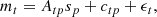
Specifically, the proposed network architecture takes N low-dimensional feature vectors αn, n ∈ ⟦1, N⟧ of size 2K as input, where N is the number of samples in the training dataset, so that the input data are initially arranged in a 2D tensor of size [N, 2K]. Input feature vectors are then projected onto a higher-dimensional subspace by means of a deep neural network with multiple deconvolutional layers1. For all feature vectors αn, n ∈ ⟦1, N⟧, a reshape operation followed by a nonlinearity, provided by a ReLU operator, converts the input data into K channels of size n0 = 2, with the result of such operation being a tensor of size [N, 2, K]. A first circular deconvolutional layer dilates these K channels into 2K channels of sizes n1 = 8. M − 2 subsequent convolutional layers further dilate these 2K channels to sizes n2 = 32, …, nm = 2 ⋅ 4m, …, nM − 1 = 2 ⋅ 4M − 1, with the corresponding results of such operations being tensors of size [N, 8, 2K],[N, 32, 2K],…,[N, 2 ⋅ 4m, 2K],…,[N, 2 ⋅ 4M − 1, 2K], respectively. A final circular deconvolutional layer combines the existing 2K channels to produce the final output of the decoder network, a 2D tensor o(n, b) of size [N, 2 ⋅ 4M]. Each of the N lines of this output tensor corresponds to one of the N low-dimensional input feature vectors αn.
Finally, a piece-wise constant interpolation scheme is used to interpolate the N network outputs of size 2 ⋅ 4M into N higher dimensional output vectors relating to observations mt. To this end, for each observation n, time-ordered data are binned into 2 ⋅ 4M bins so that all data points corresponding to bin b in observation n are interpolated as o(n, b). The binning strategy for this final step is directly dependent on the considered problem and dataset. For Planck-HFI 545 GHz data, this binning is detailed in Sect. 3. A schematic representation of the network structure is presented in Fig. 2.
 |
Fig. 2. Considered Decoder CNN architecture. |
As previously explained, neural-network-based dimensionality reduction is classically performed by exploiting autoencoders, which usually involve deep symmetrical architectures with a bottleneck central layer providing the low-dimensional representation. This is achieved by using observations as both input and output at training, so that the considered network learns the optimal low-dimensional representation space that minimizes reconstruction error. However, in the proposed approach, we rather exploit an input-training scheme to avoid training an encoder network. Input training is achieved by optimizing the network input, in our case the low-dimensional representation αn, alongside the remaining network parameters. Provided that the considered loss function is differentiable with respect to inputs, classic neural-network training approaches can be used to backpropagate gradients through the input layer and optimize the inputs themselves.
2.2.1. Custom loss function
In our framework, we wish to ensure an efficient separation between the spatial signal sp and the large-scale systematic effects ctp modeled by the proposed neural-network architecture. To this end, we follow classic mapmaking approaches and, under the hypothesis that the projected spatial signal Atpsp for any given pixel p remains constant in time, we exploit spatial redundancy in observations mt, provided by spatial crossings or co-occurrences in observations at different times, to remove signal sp from observations mt. For a given pixel p, this means computing the mean observation Mp and subtracting it from any and all observations mt corresponding to pixel p:
 (2)
(2)
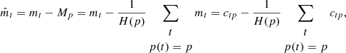 (3)
(3)
where p(t) designates the pixel corresponding to observation mt at time t, and H(p), known as the hit-count, is the total number of observations at pixel p.
In the proposed decoder-network-based approach, observations mt are used for training by considering the output of the decoder network to provide a parametrization of large-scale systematic effects:
 (4)
(4)
so that the network, including its inputs αn, can be trained to minimize reconstruction error with respect to signal free observations  . The appropriate training loss function can then be directly derived from Eqs. (3) and (4):
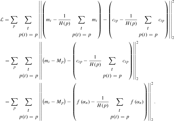 (5)
(5)
From Eqs. (3)–(5), it can be concluded that the time invariance hypothesis of projected spatial signal Atpsp ensures that all traces of signal sp can be adequately removed from observations mt during the data inversion. Even though this hypothesis may not always be formally respected depending on the considered dataset and application, it still remains a valid approximation for a large number of applications, provided that the appropriate spatiotemporal scales and sampling frequencies for observations are chosen.
Following recent trends in machine learning (Raissi et al. 2017a,b, 2018; Karpatne et al. 2017; Lusch et al. 2018; Nabian & Meidani 2018; Raissi & Karniadakis 2018; Yang & Perdikaris 2018, 2019; Erichson et al. 2019; Lutter et al. 2019; Roscher et al. 2020; Seo & Liu 2019), we designed a custom loss function including a standard reconstruction error term (as in most machine learning applications) coupled with physically derived terms introducing expert knowledge relating to the application and dataset considered (see Sect. 3 for detailed examples).
2.2.2. 2D Decoder CNN alternative formulation
Besides the previously introduced Decoder CNN architecture, we propose an alternative 2D formulation of the original Decoder CNN. The novel 2D formulation amounts to modifying the network so that the intermediate convolutional layers involve 2D convolutional kernels. In this regard, this alternative formulation relies on a 2D binning of observations mt for training. In particular, here we exploit a fully connected layer to allow us to considerably reduce the dimension of the low-dimensional representation of the signals of interest at the expense of increasing the number of weights and biases to be learned during training. Contrary to a convolutional layer, which involves a convolution where each value of the produced multidimensional output depends only on a local subset of a multidimensional input (due to the convolution operation), a fully connected layer produces the output by means of a linear combination of all values in the input. In a fully connected layer, the weights and biases to be learned are those of the linear combination that produces the output. This implies that trainable inputs, that is, the low-dimensional representation, αn, n ∈ ⟦1, N⟧ of size K should now be arranged into a 2D tensor of size [N, K], which will be converted by a fully connected layer into K channels of size [2, 2], with the result of such an operation being a tensor of size [2, 2, K]. A first convolutional layer further expands this tensor into 2K channels, producing an output of size [8, 8, 2K]. In a similar fashion to the original Decoder CNN, M − 2 subsequent circular deconvolutional layers dilate these 2K channels along the first two dimensions into sizes n1 = 8, n2 = 32, …, nm = 2, ⋅4m, …, nM − 1 = 2 ⋅ 4M − 1, with the corresponding results of such operations being tensors of size [8, 8, K],[32, 32, K],…,[2 ⋅ 4m, 2 ⋅ 4m, K],…,[2 ⋅ 4M − 1, 2 ⋅ 4M − 1, K], respectively. A final circular deconvolutional layer combines the existing 2K channels to produce a tensor of size [2 ⋅ 4M, 2 ⋅ 4M].
Finally, a piece-wise constant interpolation scheme is used to interpolate the network outputs of size [2 ⋅ 4M, 2 ⋅ 4M] into outputs corresponding to observations mt. To this end, time-ordered data is binned two-dimensionally into (2 ⋅ 4M)×(2 ⋅ 4M) bins. The binning strategy for this final step is directly dependent on the considered problem and dataset. A schematic representation of the network structure is presented in Fig. 3.
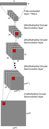 |
Fig. 3. Considered 2D Decoder CNN architecture. |
2.3. Map constraint
Given that the proposed approach exploits spatial redundancy in the observations by minimizing loss function (5), which is computed on observation co-occurrences only, no strong constraint is imposed on the large-scale signature of the network output. In this regard, the network output may, in some cases, resort to adding a large-scale signal that remains close to zero around the ecliptical poles where most signal crossings occur in order to further minimize the loss function. As few crossings exist in between the ecliptical poles, this large-scale signal will not be adequately constrained by observations and will rarely produce a physically sound reconstruction. To prevent such behavior, the following additional constraint on the final correction map, given by  is considered:
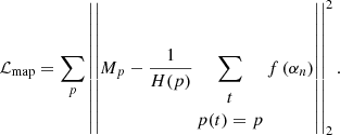 (6)
(6)
Such a constraint will penalize solutions where the final correction map diverges from the input map, thus avoiding the inclusion of a strong large-scale signature on the network correction.
The compromise between the original loss function (5) and the additional map constraint (6) is controlled by means of a user-set weight Wmap, so that the final modified loss function is given by:
 (7)
(7)
2.4. Transfer learning
In the context of the processing of Planck-HFI observations, transfer learning techniques are of particular interest given the limited amount of data available. This is in perfect agreement with the main motivation behind transfer learning, which aims to leverage knowledge from previously learned models to tackle new tasks, thus going beyond specific learning tasks and domains to discover more general knowledge shared among different problems. As illustrated below, transfer learning allows us to do this using data from different bandwidths and by exploiting different detectors to complement each other and produce more accurate sky maps.
To further constrain the proposed decoder network, particularly for identifying and removing contamination sources shared among multiple detectors, we explore classic transfer learning techniques. As previously explained, transfer learning relies on learning and storing knowledge from a particular problem or case study and applying such knowledge to solve a similar but different problem or case study.
Given the specificities of the proposed Decoder CNN architecture, we train the whole network on a source task and only retrain the low-dimensional representation (i.e., the low-dimensional inputs αn) on the target task. Such an approach can be seen as a particular case of feature-representation transfer learning (Pan & Yang 2009), because the knowledge transferred between tasks lies in the way the signals and processes of interest are represented in the low-dimensional subspace of the inputs. Indeed, as we may consider the Decoder CNN as a projection of the observations onto the low-dimensional space of the inputs, transferring the network weights and biases and only retraining the inputs amounts to considering that the projection onto the space of the inputs is shared between the two learning tasks considered. This means that the source learning task will learn a projection, defining a low-dimensional representation, which will then be used as is by the target task.
In the context of the proposed application, we exploit transfer learning to better learn structured large-scale systematic effects by training the proposed Decoder CNN on a dataset accurately depicting these large-scale systematic effects. Given that we focus on learning the projection that most accurately captures the structure of large-scale systematic effects, the Decoder CNN is trained on the whole dataset rather than on observation co-occurrences (as is done with cost function (5)), which amounts to considering the following training cost function:
 (8)
(8)
After training, the resulting Decoder CNN is transferred to a new dataset, which amounts to retraining the Decoder CNN inputs only using the original cost function (Eq. (5)), while keeping the previously trained weights and biases.
In this context, two distinct cases can be discerned. The first case involves two detectors that measure the sky signal in the same frequency band, while the second case involves two detectors measuring the sky signal on different frequency bands. Both cases rely on training the Decoder CNN on a dataset from a specific detector, and then retraining inputs only on a different dataset pertaining to a different detector. As the learning tasks for both detectors are different (the considered cost functions are different), such a procedure effectively amounts to transfer learning. This is further reinforced if the second detector dataset differs significantly from the first detector dataset, that is, if we choose, for example, to train the Decoder CNN on a 545 GHz detector dataset and retrain the inputs using a 857 GHz detector dataset. The simpler case where both detectors measure the sky signal in the same frequency band still amounts to transfer learning, but may involve more accurate knowledge transfer, given the strong similarities between the source and target datasets.
3. Planck-HFI case study
3.1. Planck observation strategy
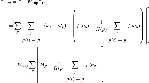
The Planck satellite scanning strategy, a clear schema of which can be found in Sect. 1.4 of Planck Collaboration ES (2018), is determined by a halo orbit around the Lagrange L2 point. The satellite rotates around an axis nearly perpendicular to the Sun (Tauber et al. 2010a) and scans the sky in nearly great circles at around 1 rpm, which means that the ecliptic poles are observed considerably more frequently, and in many more directions, than the ecliptic equator. Thus, ecliptic poles concentrate most of the observation crossings and co-occurrences providing the required redundancy to ensure effective separation and removal of large-scale systematic effects. This can be clearly observed in Fig. 4, where we present a Planck-HFI 545 GHz channel hit-count map, that is, the number of observations at each pixel.
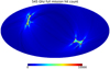 |
Fig. 4. Full-mission observation hit-count map, that is, the total number of observations at each pixel, for the Planck-HFI 545 GHz channel. |
The redundancy pattern produced by the Planck-HFI scanning strategy is particularly relevant for our approach, given that the network training takes spatial redundancy into account for the removal of signal sp to ensure that the CNN is trained to capture and model large-scale systematic effects ctp = f(αn) only. In this regard, the choice of a scanning strategy is a critical point in the design of most remote sensing satellite missions, as it determines a compromise between spatial redundancy (necessary for accurate removal of spatially redundant sources of contamination) and spatiotemporal sampling resolution (necessary to obtain accurate and reliable measurements of the signal of interest). For most remote-sensing satellite mission designs, the choice of scanning strategy is usually the product of extensive research based on multiple end-to-end simulations of the observing system.
3.2. Planck data preprocessing and compression
Time-ordered data from the Planck satellite are sampled in consecutive 1 rpm rotations of the satellite. These observations can be naturally organized into discrete packages, with measurements corresponding to each full rotation being grouped together into units called circles. Given the relationship between the rotational velocity of the satellite and its orbital velocity around the Sun, consecutive circles can be grouped together every 60 rotations and averaged to produce a composite measurement, called a ring, under the approximation that the region of the sky observed by 60 consecutive circles (∼1 hour) remains constant.
Given that a ring corresponds to 60 averaged rotations at a constant angular velocity, the sampling frequency of the instrument then determines a uniform sampling of the phase space within each ring. In this way, the phase of a full rotation is discretized into B points, so that each measurement in a ring corresponds unequivocally to a phase bin of amplitude  .
.
Further compression of the information present in the Planck-HFI 545 GHz and 857 GHz datasets is achieved by considering a HEALPix pixelization (Górski et al. 2005) with Nside = 2048 and averaging, for each ring, all measurements that fall within the same pixel. As far as phase information is concerned, each new averaged measurement is associated with a composite phase value obtained by averaging the phase of all measurements falling within the considered pixel. In this way, phase information loss due to averaging, and the associated subpixel artifacts (i.e., inconsistent pixel values related to the loss of phase information) are minimized. As the considered compression stage produces results of varying length depending on each ring’s orientation with respect to the pixelization grid, zero padding is used to produce a homogeneous dataset by converting the length of all rings to l = 27 664, which is the length of the largest compressed ring in the dataset.
3.3. Far side lobe pickup large-scale systematic effect
For the application considered in the present work, we focus specifically on one large-angular-scale systematic effect, namely the FSL pickup, which consists of radiation pickups far from the Planck telescope line of sight, primarily due to the existence of secondary lobes in the telescope’s beam pattern, which creates what is commonly known as “stray-light contamination” (Tauber et al. 2010b; Planck Collaboration III 2016). Regarding the FSL data used for the present study, we consider simulation data obtained using a customized and improved variant of the GRASP simulation tool (Tauber et al. 2010b). The interested reader can find full implementation details of these simulations in Tauber et al. (2010b). Particularly, Fig. 5 of Tauber et al. (2010b) includes a depiction of a typical FSL pattern obtained using this method. Typically, FSL pickup is characterized by a highly structured large-angular-scale signature, which makes it an ideal candidate to evaluate the proposed method’s ability to exploit such structure to project the signals of interest onto a low-dimensional subspace where such structured information is adequately represented with a reduced number of degrees of freedom. In this regard, we focus our analysis on larger spatial scales (below multipole ℓ = 100, that is, angular scales over 1°), given that FSL pickup is primarily a large-scale systematic effect. Moreover, the dominant contamination source at small scales in Planck-HFI data is the detector noise, which can be modeled as an unstructured Gaussian signal that cannot be effectively removed by the proposed method, which further motivates our choice to focus on large spatial scales. However, it should be noted that even though we focus here on the FSL pickup, other structured contamination sources present in intermediate spatial scales not yet dominated by detector noise may also be removed with the proposed methodology, but this is beyond the scope of this work.
3.4. Planck-HFI 545 GHz dataset
To illustrate the relevance of the framework introduced in Sect. 2, we consider synthetic simulation data from the Planck-HFI 545 GHz dataset of the Planck mission (Tauber et al. 2010a). As previously explained, the choice of the Planck-HFI 545 GHz channel is motivated by its weak CMB signature, which simplifies both the data processing and the interpretation of obtained results. In particular, we exploit FSL pickup synthetic 545 GHz data to validate the ability of our method to learn suitable low-dimensional representations of the FSL pickup under both ideal and nonideal settings, including cases considering incomplete, gap-filled, and inconsistent datasets.
3.5. Planck-HFI 857 GHz dataset
Besides Planck 545 GHz synthetic simulation data, we also consider Planck 857 GHz real observation data to evaluate how data augmentation techniques can be exploited to improve the contamination source removal performance of the Decoder CNN architecture, as explained in Sect. 4.2. Similarly to the Planck-HFI 545 GHz channel, the Planck-HFI 857 GHz channel presents a weak CMB signature, which simplifies both the data processing and the interpretation of obtained results. This implies that the detector difference maps between different detectors will predominantly depict large-scale systematic effects, with the FSL pickup being the dominant systematic observed (Planck Collaboration III 2020). As such, Planck-HFI 857 GHz real observation data provide an ideal setting to evaluate the ability of the proposed method to capture and remove large-scale systematic effects, and especially the FSL pickup. Importantly, the Planck-HFI 857 GHz channel has the particularity that, given the position of its associated detectors on the focal plane, detector 8572 presents very little FSL pickup.
Moreover, the considered Planck 857 GHz dataset shares many similarities with the previously introduced Planck 545 GHz dataset, including the circle-averaging used to produce rings and the HEALPix pixelization-based information compression (presented in Sect. 3.2). Besides the difference in frequency bands, the main difference lies in the slightly different observation spatial distribution produced by the differences in location and orientation of the detectors involved. Specifically, the considered dataset corresponds to real calibrated data from the 2018 Planck release (available at the Planck Legacy Archive2), which implies several preprocessing steps have already been performed on the dataset, such as cosmic-ray-glitch removal and transfer-function correction at the time-ordered data level, among others. This implies that, besides the FSL signal, other systematic effects (CMB solar dipole, calibration discrepancies between detectors, etc.) are also present. The SRoll algorithm takes into account most of these residual systematic effects using templates. Thus, for the 857 GHz channel, many such residual sources of contamination are either considerably weak with respect to the FSL residual signal, as seen in the differences between detector maps, or not relevant at the large scales considered (as is the case, most notably, for cosmic-ray glitches).
3.6. Decoder network training
Taking Planck-HFI 545 GHz and 857 GHz data specificities into consideration for the proposed decoder-network-based approach, we chose to train our decoder network on compressed rings directly, so that the final step of the decoder network, considering M = 3, uses a piece-wise constant interpolation to interpolate l = 27 664 values from the 2(43) = 128 larger bins produced as output by the decoder network. Using phase values as the independent interpolation variable, network outputs are thus interpolated to length l = 27 664, and compared to compressed rings during training. Network parameters and inputs are jointly optimized in order to minimize reconstruction error while ensuring the effective removal of large-scale systematic effects by minimizing the custom loss function (Eq. (5)). Moreover, an additional map constraint term, as introduced in Sect. 2.3, is added to the loss function (Eq. (5)) to introduce physics-informed constraints and leverage domain knowledge on the inversion problem. Finally, transfer learning strategies, as presented in Sect. 2.4, are also explored as a means to share and transfer relevant information between datasets.
4. Results
4.1. Validation on 545 GHz FSL simulations
We explore the ideas introduced in Sect. 3 by training our Decoder CNN on FSL simulation data from a 545 GHz detector (detector 5451). For the considered case study, data from all Planck-HFI 545 GHz detectors was considered. The proposed method was applied to each detector individually, with similar results being obtained. For the sake of simplicity, only results for detector 5451 are presented. Given that we focus here on evaluating the capacity of neural-network-based representations to accurately depict large-scale systematic effects, we do not consider, for the validation stage, multidetector approaches combining data from several sources. However, it should be noted that the SRoll algorithm was originally developed in a multidetector setting. Further tests considering multiple detectors were not considered for the validation stage, as we consider them to be beyond the scope of our validation objectives. As we further underline in our conclusions, this does nonetheless remain an interesting avenue to further explore the potential of neural-network-based approaches and transfer-learning strategies in the context of the removal of large-scale systematic effects. The objective of this validation stage is to demonstrate the ability of the method to adequately learn a suitable low-dimensional representation for the signals of interest from data. In this regard, the learned representation embeds knowledge learnt from the available dataset that facilitates the separation and removal of structured large-scale systematic effects (provided that such knowledge effectively exists within the dataset), while also being optimized with respect to the data inversion itself. Moreover, transfer-learning techniques are evaluated using phase-shifted data from the same detector. As Planck-HFI datasets are binned in phase, phase shift amounts to a simple circular shift operation at the ring level, so that all rings are shifted a fixed number of bins bs and overflowing bins at one end are reintroduced into the ring at the other end. The number of bins bs to be shifted is determined as a function of the number of bins used for phase binning B and the desired shift angle αs:  . In this regard, considering phase-shifted data allows us to simulate either partially similar detector datasets, and/or cases where the FSL pickup is partially or poorly modeled. It should be noted that phase-shifted data is purely exploited as a means to emulate missing knowledge within the training dataset. In this regard, the considered phase shift is not necessarily a representation of the real physical phenomena occurring within the satellite’s optical system, but it is rather a simplified scheme to demonstrate how the proposed inversion method responds to training on incomplete or inconsistent datasets. Indeed, one may consider introducing a phase shift in data as a simple means to distort the learning dataset, thus simulating either acquisition errors or the use of data from a different detector for the network training. This is particularly relevant for the Planck mission, given that different detectors have slightly different positions in the satellite’s focal plane, which can be modeled, albeit in a simplified way, by phase shifts in data. In this regard, among the tests considered, we include a direct fit, as a template, of phase-shifted data onto nonshifted data. We expect this fit to emulate the result we would obtain if the direct fit technique exploited by the original SRoll2 algorithm was used to fit and remove distorted data (either by acquisition errors or differences in focal plane position) from nondistorted data. This result is used primarily for comparison and benchmarking purposes as a ground-truth reference to evaluate the gain obtained when exploiting our proposed methodology, with respect to the original SRoll2 approach. All considered datasets consist of 747 093 984 observations packed into rings of size 27 664, for a total ring count of N = 27 006 rings.
We evaluate performance by presenting and comparing results obtained for the following approaches:
-
A classic destriping (Planck Collaboration VIII 2016) of detector 5451 FSL simulation data (referred to as CD hereafter).
-
A direct fit of a FSL template computed from 20° phase-shifted detector 5451 FSL simulation data onto detector 5451 FSL simulation data (referred to as TFIT hereafter).
-
The Decoder CNN in its original one-dimensional (1D) version trained and applied directly on detector 5451 FSL simulation data (referred to as CNN1D hereafter).
-
The Decoder CNN in its original 1D version trained and applied directly on detector 5451 FSL simulation data and considering an additional weighted map constraint (referred to as CNN1D-Wmap hereafter).
-
The Decoder CNN in its original 1D version trained on 20° phase-shifted detector 5451 FSL simulation data and applied to nonshifted detector 5451 FSL simulation data by retraining inputs only (referred to as CNN1D-TL hereafter).
Subsequently, we also perform additional tests to evaluate:
-
the performance of the 2D alternative formulation of the Decoder CNN for the original case studies and datasets (referred to as, respectively, CNN2D, CNN2D-Wmap and CNN2D-TL hereafter);
-
the performance of the proposed algorithms when applied to a gap-filled dataset generated by subsampling available observations.
For comparison and benchmarking purposes, we include, among the methods considered, a classic destriping approach. This result is used as a baseline for evaluating the performance of the proposed methodology. For the considered methods, results are evaluated qualitatively by means of final full-mission-output maps and half-mission-difference maps, which are presented for visual comparison.
Regarding the processing of Planck-HFI data, several ways of splitting the datasets for their analysis are described in Planck Collaboration III (2020). Here, we use half-mission-difference maps, which are computed by dividing the whole time-ordered data-series in two equal halves, processing each half independently and then computing the difference between the obtained maps. As such, half-mission-difference maps remove all spatially redundant information, allowing analysis of the information remaining once structured spatial signals are removed. This implies that half-mission-difference maps provide relevant information regarding the training of the Decoder CNN, because it is trained using a custom cost function that explicitly removes redundant spatial information, but they do not provide much information regarding the real performance of contamination-source removal.
Moreover, a quantitative performance evaluation is given by means of the power spectra of the presented maps, which are computed using a spherical harmonics decomposition. In this spectral representation, multipole scale number ℓ relates to different spatial angular scales. As such, the power spectra depict how energy is distributed across angular scales, thus providing a multiscale measurement of the power per surface unit within the analyzed map.
4.1.1. One- and two-dimensional Decoder CNNs
The first considered case study involves exploiting data from the Planck-HFI 545 GHz channel only. In this context, transfer learning amounts to training the Decoder CNN on phase-shifted data from detector 5451, and exploiting this network to process nonshifted data from detector 5451 by retraining inputs only. As previously stated, such an approach can be considered as transfer learning despite the similarities between the two datasets, because the source and target learning tasks are different.
For the considered case study, the 1D Decoder CNN considers K = 4 channels and M = 3, meaning that the 1D Decoder CNN architecture uses four deconvolutional layers to project a total number of 8N inputs onto time-ordered data binned into 128 phase bins. For the map-constrained version of the Decoder CNN (trained with loss function (7)), we consider Wmap = 10−2, which was chosen empirically as it produced the best results when testing the sensitivity of the method to this parameter, evaluated quantitatively by means of the final half-mission-map-difference power spectra.
We further complement our performance study by analyzing and comparing results obtained by contamination-source removal from FSL simulation data with the 2D variants of the Decoder CNN introduced in Sect. 2.2.2. To this end, we exploit a 2D Decoder CNN to process 545 GHz data under identical conditions to those analyzed for the 1D Decoder CNN. In this regard, the results for the 2D CNN Decoder were also obtained by considering K = 4 and M = 3, meaning that the considered 2D Decoder CNN consists of four 2D deconvolutional layers and will project 16 (4 × 4) inputs onto time-ordered data vectors binned into 128 × 128 bins in phase and time. For the map-constrained version, user-set weight Wmap is once again set to Wmap = 10−2.
Figure 5 presents, for the different considered approaches, the power spectra of the full-mission maps and the half-mission-difference maps for the different variants considered. For a qualitative analysis of these results, Fig. 6 presents these full-mission and half-mission-difference maps themselves. Additionally, Figs. 5 and 6 also include maps, and their corresponding power spectra, for the best result obtained when exploiting the 2D formulation of the Decoder CNN, that is, for CNN2D-TL (exploiting CNN weights and biases learnt on 20° phase-shifted detector 5451 FSL simulation data). For the sake of simplicity and readability, the lesser performing variants of the 2D formulation are not included in Figs. 5 and 6. Moreover, as we consider idealized synthetic simulation data here, numerical results have no real physical interpretation, and are therefore presented using arbitrary units.
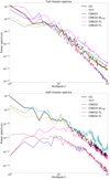 |
Fig. 5. Power spectra (in arbitrary units) of full-mission maps (top) and half-mission-difference maps (bottom) of detector 5451 FSL simulations after contamination-source removal using 1000 iterations of a classic destriping approach (CD), a direct fit of 20° phase-shifted detector 5451 FSL simulation data as a template (TFIT), the original 1D Decoder CNN (CNN1D), the 1D Decoder CNN variants using the additional map constraint (CNN1D-Wmap) and transfer learning by training the Decoder CNN weights and biases on 20° phase-shifted data from detector 5451 FSL simulations (CNN1D-TL), and the 2D variant of the Decoder CNN using transfer learning by training the Decoder CNN weights and biases on 20° phase-shifted data from detector 5451 FSL simulations (CNN2D-TL). |
 |
Fig. 6. Full-mission and half-mission-difference maps (in arbitrary units) of detector 5451 FSL simulations after contamination-source removal using 1000 iterations of a classic destriping approach (CD), a direct fit of 20° phase-shifted detector 5451 FSL simulation data as a template (TFIT), the original 1D Decoder CNN (CNN1D), the 1D Decoder CNN variants using the additional map constraint (CNN1D-Wmap), and transfer learning by training the Decoder CNN weights and biases on 20° phase-shifted data from detector 5451 FSL simulations (CNN1D-TL), and the 2D variant of the Decoder CNN using transfer learning by training the Decoder CNN weights and biases on 20° phase-shifted data from detector 5451 FSL simulations (CNN2D-TL). Leftmost columns present full-mission maps, rightmost columns present half-mission-difference maps. |
Concerning the 1D variants of the Decoder CNN, Fig. 5 shows that both CNN1D and CNN1D-Wmap provide a substantial gain for the filtering of smaller scale FSL structures, while not being able to accurately remove the large-scale FSL signature. However, CNN1D obtains the best performance in terms of large-scale contamination source removal (at multipole ℓ = 0). CNN1D-TL (trained on a phase-shifted detector dataset) degrades performance overall, while TFIT provides the best results at larger scales while not being able to capture smaller scale structures. As far as the 2D variant of the Decoder CNN is concerned, it seems that CCN2D-TL shows considerable improvement in terms of performance in contamination-source removal for larger spatial scales, even outperforming TFIT. For smaller spatial scales, however, the use of CNN2D-TL does not seem to provide any performance gain, with respect to CD, and may even degrade performance for larger ℓ values. Similarly, from Fig. 5, one can observe a considerable gain for all spatial scales in the half-mission difference maps when considering CNN1D and CCN1D-Wmap. Globally, CNN1D seems to provide the most substantial gain for most spatial scales. In agreement with these findings, the half-mission-difference map for CNN1D is less energetic and closer to a Gaussian white noise in space (even though some residual signal can still be observed) than the other analyzed Decoder CNN variants. However, the use of CNN1D-TL does seem to provide some gain for all spatial scales, even though it is marginal when compared to CNN1D and CNN1D-Wmap, especially for smaller spatial scales. TFIT produces an even smaller performance gain, remaining quite close to the performance levels of CD, while CNN2D-TL appears to be the worst performing variant overall for half-mission-difference-map contamination-source removal. Indeed, CNN2D-TL, the best performing 2D variant of the Decoder CNN, does not seem to provide any significant performance gain for half-mission-difference-map contamination-source removal, with a slightly worse performance level than TFIT at larger spatial scales, and a clear degradation in performance of contamination-source removal with respect to a CD for smaller spatial scales. Overall, the half-mission-difference maps are in strong agreement with this analysis.
Given that previous results showed little degradation in terms of half-mission-difference-map contamination-source removal, results presented in the following sections focus specifically on the performance of contamination-source removal for full-mission maps. Moreover, for the sake of readability, we focus exclusively on a quantitative analysis by means of power spectral plots, and do not include additional map plots.
4.1.2. Partial observations with large gaps
To further illustrate the relevance of transfer-learning techniques, we now consider the previously introduced Planck-HFI 545 GHz dataset but subsample one every ten rings, which amounts to considering a partial dataset involving large gaps. We consider an identical configuration for the considered Decoder CNN to the one used for previously presented results, namely K = 4 channels and M = 3, for a total of 128 phase bins for the 1D Decoder CNN and 128 × 128 bins in phase and time for the 2D Decoder CNN. For the map-constrained versions of the Decoder CNN, Wmap is kept at its original value of Wmap = 10−2.
We present similar results to those introduced in Sect. 4.1; that is, full-mission map power spectra in Fig. 7. Our initial analysis of the obtained results indicates that, given the large gaps in the considered dataset, the Decoder CNN tends to add a considerable spatial offset to the whole map in order to fill in those gaps. During our tests, this effect was partially limited by the additional map constraint, even though this does suffice to completely remove the offset. From the full-mission maps before removing offsets, we observed that both CNN1D and CNN1D-Wmap were unable to correctly capture and filter the FSL signal. CNN1D-TL on the other hand considerably improves performance when considering partial datasets involving large gaps, most notably for smaller spatial frequencies.
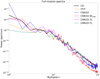 |
Fig. 7. Power spectra (in arbitrary units) of full-mission maps of detector 5451 FSL simulations considering one in every ten rings after contamination-source removal using 1000 iterations of a classic destriping approach (CL), a direct fit of 20° phase-shifted detector 5451 FSL simulation data as a template (TFIT), the original 1D Decoder CNN (CNN1D), the 1D Decoder CNN variants using the additional map constraint (CNN1D-Wmap) and transfer learning by training the Decoder CNN weights and biases on 20° phase-shifted data from detector 5451 FSL simulations (CNN1D-TL), and the 2D variant of the Decoder CNN using transfer learning by training the Decoder CNN weights and biases on 20° phase-shifted data from detector 5451 FSL simulations (CNN2D-TL). |
After subtracting the spatial mean, we observe that performance is considerably improved, particularly for CNN1D-TL, which, among all 1D Decoder CNN variants, produces the best results for larger spatial scales, closely followed by CNN1D-Wmap, which also presents the best overall performance for smaller scales. On the other hand, CNN1D is poorly suited to handling incomplete datasets involving large gaps, as can be concluded by its subpar performance with respect to CNN1D-Wmap and CNN1D-TL. Similarly to previous results, none of the 1D variants are capable of outperforming TFIT, which does indeed present a better contamination source removal performance for large spatial scales. CNN2D-TL on the other hand outperforms TFIT for larger spatial scales, at the expense of a slightly worse contamination-source-removal performance than that of CD for smaller spatial scales.
4.1.3. Transfer learning for phase-shift correction
To further illustrate the relevance of transfer-learning strategies for improving the characterization of large-scale systematic effects, we consider a case study involving 545 GHz FSL simulations with additional phase-shift values. The primary objective is to evaluate the ability of the proposed approach to extract knowledge from an incomplete or inconsistent dataset that nonetheless contains relevant information that may be exploited to learn a suitable low-dimensional representation of the signals of interest. As previously explained, considering phase-shifted data at different phase shift values allows us to emulate both partially similar detectors and inaccurate FSL templates. As such, a phase-shifted version of the original FSL simulation is exploited to learn the Decoder CNN weights and biases, which are then applied to the mapmaking and contamination source removal of the original FSL simulation. Moreover, we also explore the possibility of combining multiple phase-shifted datasets as a means to construct an enriched dataset that better represents the relevant information to be learnt by the CNN. To this end, the weights and biases computed from the 20° phase-shifted FSL data are fixed, and only the low-dimensional inputs are retrained on the original (nonshifted) FSL observations.
We evaluate performance by presenting and comparing results obtained for the following approaches:
-
a classic destriping of 5° phase-shifted detector 5451 FSL simulation data (referred to as CD5 hereafter);
-
a direct fit of a FSL template computed from nonshifted detector 5451 FSL simulation data onto 5° phase-shifted detector 5451 FSL simulation data (referred to as TFIT0 → 5 hereafter);
-
the Decoder CNN in its original 1D version trained on nonshifted detector 5451 FSL simulation data and applied to 5° phase-shifted detector 5451 FSL simulation data by retraining inputs only (referred to as CNN1D0 → 5 hereafter);
-
the Decoder CNN in its 2D version trained on nonshifted detector 5451 FSL simulation data and applied to 5° phase-shifted detector 5451 FSL simulation data by retraining inputs only (referred to as CNN2D0 → 5 hereafter);
-
the Decoder CNN in its 2D version trained on a catalog built from detector 5451 FSL simulation data shifted by [6° ,8° ,…,18° ,20° ] and applied to 5° phase-shifted detector 5451 FSL simulation data by retraining inputs only (referred to as CNN1D[6, 20]→5 hereafter);
-
the Decoder CNN in its 2D version trained on a catalog built from detector 5451 FSL simulation data shifted by [0° ,2° ,…,18° ,20° ] and applied to 5° phase-shifted detector 5451 FSL simulation data by retraining inputs only (referred to as CNN1D[0, 20]→5 hereafter).
Given that we are interested in evaluating the potential of the transfer-learning-based 2D Decoder CNN to accurately learn the shape of FSL pickups, all considered networks rely on a single input for the low-dimensional representation of the signals of interest. The principle behind such an architecture is that the CNN weights and biases will capture the overall shape of FSL pickups, which implies that the free low-dimensional input should capture the phase shift between the different datasets considered. As such, we consider an asymmetrical variant of the 2D Decoder CNN, such that the two dimensions of the network output can be of different sizes. This choice allows us to have a better control over the quantization of the spatial and temporal binnings considered. The 2D architecture consists of an initial fully connected layer that projects a single input onto K = 32 channels to produce a tensor of size [1, 42, 2 ⋅ 41, 32], followed by M − 1 2D deconvolutional layers to dilate these K channels and produce tensors of sizes [16, 8, K],[64, 32, K],…,[4m + 1, 2 ⋅ 4m, K],…,[4M + 1, 2 ⋅ 4M, K], respectively. A circular deconvolutional layer then combines the existing K channels to produce a tensor of size [4M + 2, 2 ⋅ 4M + 1]. For training, time-ordered data are binned into 4M + 2 × 2 ⋅ 4M + 1 bins in ring and phase space, respectively, to match the network output.
For the present case study, we consider M = 3, meaning that the proposed network outputs relies on a 1024 × 512 binning of time-ordered data in ring and phase space. We present similar results to those introduced in previous sections, that is, full-mission power spectra in Fig. 8.
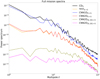 |
Fig. 8. Power spectra of full-mission maps of 5° phase-shifted detector 5451 FSL simulations after contamination-source removal using 1000 iterations of a classic destriping approach (CD5), a direct fit of nonshifted detector 5451 FSL simulation data onto 5° phase-shifted detector 5451 FSL simulation data as a template (TFIT0 → 5), the 1D Decoder CNN trained on nonshifted detector 5451 FSL simulation data and applied to 5° phase-shifted detector 5451 FSL simulation data (CNN1D0 → 5), the 2D Decoder CNN trained on nonshifted detector 5451 FSL simulation data and applied to 5° phase-shifted detector 5451 FSL simulation data (CNN2D0 → 5), the 2D Decoder CNN trained on a catalog built from detector 5451 FSL simulation data shifted by [6° ,8° ,…,20° ] and applied to 5° phase-shifted detector 5451 FSL Simulation data (CNN2D[6, 20]→5), and the 2D Decoder CNN trained on a catalog built from detector 5451 FSL simulation data shifted by [0° ,2° ,…,20° ] and applied to 5° phase-shifted detector 5451 FSL simulation data (CNN2D[0, 20]→5). |
From Fig. 8, we conclude that CNN1D0 → 5 is only able to marginally improve performance of contamination-source removal (with respect to CD5) for smaller spatial scales. This is expected, as the 1D variant of the Decoder CNN processes each ring independently and thus has a limited potential to model 2D information, which appears to be essential for the accurate capture and modeling of the phase difference to be transferred between the datasets involved. CNN2D0 → 5 performs similarly to TFIT0 → 5, and both approaches provide a significant improvement in terms of performance of contamination-source removal at all spatial scales. Such a result is explained by the fact that, as the CNN was trained on nonshifted data, it is unable to model phase shifts, as these phenomena are not accurately represented in the training dataset. Indeed, performance of contamination-source removal is considerably increased when CNN2D[6, 20]→5 is considered, which further supports the fact that the inclusion of phase-shifted data is necessary to ensure that the trained CNN learns to accurately represent phase shifts. Performance of contamination-source removal, particularly for larger spatial scales, is further improved with CNN2D[0, 20]→5, when additional phase-shifted data (between 0° and 4°) are considered. This is to be expected, as deep neural networks perform well for interpolation, but lack the necessary information to have similar performance for extrapolation. Adding phase-shifted data for smaller phase shift values means that the 5° phase shift of the target dataset is now within the phase-shift training range, and the trained network is better able to model such phase shifts.
4.2. Application to 857 GHz data
Following the validation of the proposed methodology on Planck-HFI 545 GHz FSL synthetic data, we evaluate its performance on real Planck-HFI 857 GHz observations. As previously explained, the Planck-HFI 857 GHz channel provides an ideal setting for evaluating the ability of the proposed approach to model and remove large-scale systematic effects, and FSL pickup in particular, given that the detector difference between the four 857 GHz detectors will mostly depict large-scale systematic effects, and predominantly the FSL pickup (Planck Collaboration III 2020). The 857 GHz dataset consists of time-ordered data from four independent detectors (named hereafter 857d, d = 1, …, 4).
In this context, we exploit the 2D variant of the Decoder CNN using a single input for the low-dimensional representation of the signals of interest. The 2D architecture is then identical to the one used to explore the potential of transfer-learning techniques to correct for phase shifts in Sect. 4.1.3, and consists of an initial fully connected layer that projects a single input onto K = 32 channels to produce a tensor of size [42, 2 ⋅ 41, K], followed by M − 1 2D deconvolutional layers to dilate these K channels to produce tensors of sizes [64, 32, K],…,[1, 4m + 1, 2 ⋅ 4m, …, [1, 4M + 1, 2 ⋅ 4M, K], respectively. A circular deconvolutional layer combines the existing K channels to produce a tensor of size [4M + 2, 2 ⋅ 4M + 1]. For training, time-ordered data are binned into 4M + 2 × 2 ⋅ 4M + 1 bins in ring and phase space, respectively, to match the network output.
We also explore the potential of data augmentation to integrate expert knowledge into the training of the Decoder CNN and thus provide enhanced modeling capabilities for the FSL pickup. To this end, the training dataset is enhanced by integrating information from all four detectors into the contamination-source-removal procedure of each individual detector. Specifically, for each detector, the training dataset is enriched by integrating the residue of detectors 8571, 8573, and 8574 with respect to detector 8572. Detector 8572 is chosen as the common base for all residues considered simply because its position in the focal plane within the detector array effectively reduces its FSL pickup. The computation of these residues is performed after the data are binned in ring and phase spaces. We consider M = 3, so that time-ordered data are initially binned into 1024 bins in ring space and 512 bins in phase space. Once datasets for the four detectors have been binned, each detector dataset is enriched by adding the residue, that is, the difference, between detector 8572 binned data and binned data from the three remaining detectors. These residues are then subjected to a thresholding procedure, such that all data whose absolute value is below a user-set threshold is set to zero. The idea behind this procedure is that the considered residues will not only contain relevant FSL pickups that can be used for training the Decoder CNN, but also other noise signals that should not be taken into account and that should ideally be filtered by the thresholding operation. As such, a coarse value for the threshold is set empirically by taking into account the noise levels within the considered dataset, and then fine-tuned by performing multiple simulations at different threshold values. Given that the threshold is user-set, this procedure can be seen as the integration of expert knowledge into the otherwise unsupervised procedure of network training. The final approach could therefore be qualified as a weakly supervised network training method. The proposed augmented datasets are used to train the Decoder CNN weights and biases (independently for each detector), with network inputs then being retrained directly on the original nonaugmented detector datasets.
As previously explained, Planck-HFI 857 GHz detector difference maps are dominated by the FSL pickup signal, which makes them an ideal gauge for the capacity of the proposed approach to remove the FSL pickup from the final maps. Taking this into account, we illustrate our results by presenting the power spectra of Planck-HFI 857 GHz detector difference maps in Fig. 9, and the Planck-HFI 857 GHz detector difference maps themselves in Fig. 10. For visualization and comparison purposes, all detector difference maps are normalized to a common baseline amplitude level, and any existing carbon monoxide (CO) difference map signatures are removed using the same template fit procedure used by SRoll2 to produce the 2018 release of the Planck-HFI sky maps. We compare results for three different cases, namely:
-
the mapmaking of Planck-HFI 857 GHz real data using a classic destriping approach (CD);
-
the mapmaking of Planck-HFI 857 GHz real data using SRoll2 (Delouis et al. 2019) to produce a direct fit of a synthetic FSL simulation as a template (referred to as SRoll2 hereafter);
-
the mapmaking of Planck-HFI 857 GHz real data using 1000 iterations of the 2D Decoder CNN exploiting data augmentation to include interdetector residuals in the learning dataset (referred to as CNN2D-DA hereafter).
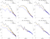 |
Fig. 9. Power spectra for detector difference maps of Planck-HFI 857 GHz real data. For all detector pairs, power spectra are computed from detector difference maps for three distinct cases: the mapmaking of Planck-HFI 857 GHz real data using a classic destriping approach (CD), the mapmaking of Planck-HFI 857 GHz real data using SRoll2 to produce a direct fit of a synthetic FSL simulation as a template (SRoll2), and the mapmaking of Planck-HFI 857 GHz real data using 1000 iterations of the 2D Decoder CNN exploiting data augmentation to include interdetector residuals in the learning dataset (CNN2D-DA). |
 |
Fig. 10. Detector difference maps of Planck-HFI 857 GHz real data. For all detector pairs, detector difference maps are computed for three distinct cases: the mapmaking of Planck-HFI 857 GHz real data using a classic destriping approach (not shown), the mapmaking of Planck-HFI 857 GHz real data using SRoll2 to produce a direct fit of a synthetic FSL simulation as a template (SRoll2, two leftmost columns), and the mapmaking of Planck-HFI 857 GHz real data using 1000 iterations of the 2D Decoder CNN exploiting data augmentation to include interdetector residuals in the learning dataset (CNN2D-DA, two rightmost columns). |
Besides detector difference maps and their corresponding power spectra, Fig. 11 presents, for illustration purposes, an example plot of the evolution of the loss function for the training of the CNN2D used to process 857 GHz channel data from detectors 8571, 8572, 8573, and 8574, as a function of the number of epochs considered (in logarithmic scale).
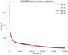 |
Fig. 11. Evolution of the loss function as a function of the epochs considered for the training of the CNN2D for detectors 8571, 8572, 8573, and 8574 (logarithmic scale). |
From the power spectra depicted in Fig. 9, we can conclude that the interdetector data augmentation strategy, coupled with the introduction of expert knowledge via the thresholding of binned data residues, allows considerable improvement in performance of contamination-source removal for all spatial scales and for most detector pairs, with a considerable gain for larger spatial scales. As such, as far as large-scale contamination-source removal is concerned, CNN2D-DA seems to outperform SRoll2 for most detector pairs. Indeed large-scale contamination-source removal performance is only marginally degraded for a single detector pair (8572 − 8574) and only for larger spatial scales (around ℓ < 20). For the remaining detector pairs, we report considerable gains, typically up to one order of magnitude, in performance in terms of contamination-source removal for large spatial scales. This demonstrates the relevance of the proposed methodology to correctly capture and remove the FSL pickup signal during the data inversion. These conclusions are further supported by the detector difference maps presented in Fig. 10, where one can observe a considerable improvement in performance of contamination-source removal for most detector pairs with respect to SRoll2 for CNN2D-DA. Interestingly, a particularly strong large-scale signal can be observed to the north of the Galactic plane, near the Galactic origin. Given that we are working with Planck-HFI 857 GHz real data, we hypothesize that this signal is caused by other contamination sources, which explains the inability of CNN2D-DA to completely remove it, as it has been extensively adapted in the presented application to deal specifically with FSL pickups.
5. Discussion
5.1. Data-driven modeling of systematic effects
5.1.1. Map constraint
As explained in Sect. 2.3, the Decoder CNN may introduce an erroneous large-scale signal to its reconstructed output. Indeed, the Decoder CNN is trained on signal co-occurrences only, and so cost function (5) may be artificially decreased by adding an adequately chosen large-scale offset, whereas the introduction of this offset does not necessarily relate to the contamination-source removal of the final map. According to our results, such a large-scale signature may appear in the form of a large-scale offset, or even higher order moments such as a large-scale spatial dipole. In particular, this was observed for results presented in Sect. 4.1, specifically for the case considering one every ten rings, that is, for partial datasets involving large gaps. This is expected, given that in such cases the lack of observations between the ecliptic poles is exacerbated, thus further strengthening this effect. As can be observed in our results, the introduction of a map constraint (Eq. (6)) helps to limit the introduction of a large-scale offset, given that it improves the network conditioning in difficult cases, such as those considering partial, gap-filled, or irregularly sampled datasets. This demonstrates both the flexibility of the proposed framework to be adapted to the dataset and/or problem to be treated by incorporating appropriate additional terms to the custom cost function (5) and its capability to adequately handle partial, gap-filled datasets.
5.1.2. Transfer learning
As observed, the exploitation of transfer-learning techniques allows the characterization of the “shape” of the large-scale systematic effects we are trying to separate from our signal of interest. This is achieved by constraining the smaller dimensional subspace onto which the considered signals are projected. The “shape” of large-scale systematic effects is indeed encoded into a projection operator, which is parameterized by the Decoder CNN by minimizing the loss function on the training dataset. The trained Decoder CNN is then applied to a second dataset by retraining the inputs only. As previously stated, this can be seen as a way of identifying and learning the common knowledge between the different datasets (i.e., the projection) and transferring such knowledge between different datasets. Such an approach is particularly relevant for applications where similar large-scale systematic effects exist between different datasets, as is the case for the FSL pickup. Indeed, in the presented application, the Decoder CNN training stage seems to learn general characteristics of the FSL pickup signal, such as its large-scale signature, which is then transferred to the second dataset (by retraining inputs) in order to improve performance in terms of contamination-source removal. From a mathematical point of view, retraining the inputs can be thought of as finding the representation in the projection subspace that best approximates the second dataset. This amounts to finding the best-fitting FSL pickup signal approximation under the constraint that the characteristics of this approximation were previously learnt from the first dataset and encoded in the Decoder CNN weights and biases.
5.2. Neural-network-based removal of large-scale systematic effects
Results obtained for Planck-HFI 857 GHz real data illustrate how data-augmentation techniques coupled with expert knowledge integration can improve performance in terms of contamination-source removal. Indeed, introducing, for each 857 GHz detector, interdetector residuals with respect to detector 8572 amounts to exploiting data augmentation to transfer relevant information between datasets. As such, this procedure is closely related to the idea of transfer learning, because both seek to exploit information shared between datasets to improve the performance of contamination-source removal. Moreover, the inclusion of a user-set threshold for interdetector binned data residues allows us to integrate expert knowledge into an otherwise completely unsupervised learning scheme. This is particularly relevant for the processing of data containing both well-known and badly modeled signals, as is the case for large-scale systematic effects present in Planck-HFI observations.
6. Conclusions
6.1. Overall summary
In the present work, we propose a neural-network-based data-inversion approach to reduce structured contamination sources, with a particular focus on the mapmaking for Planck-HFI data and the removal of large-scale systematic effects within the produced sky maps. The proposed approach relies on a generative decoder convolutional neural network to project the signals of interest onto a low-dimensional subspace learnt simultaneously with a data inversion, so that the low-dimensional subspace is optimized with respect to the contamination-source removal and mapmaking objectives. This optimization is achieved by means of a loss function that takes such objectives into account during the network-training stage. The exploitation of such a custom loss function also allows the introduction of physics-based constrains to further improve the performance of contamination-source removal. The low-dimensional subspace learning is possible thanks to an input-training scheme, which also allows incomplete and/or gap-filled datasets to be processed. We propose multiple variants of the proposed approach: a 2D version capable of taking time dependencies into account, and variants exploiting transfer learning, data augmentation, and the introduction of expert knowledge to further improve reconstruction performance. Importantly, the proposed method is capable of exploiting spatiotemporal scale couplings within contamination sources to learn, simultaneously with the data inversion, a low-dimensional representation that facilitates the removal of these contamination sources. Whereas this is illustrated here with an example considering Planck-HFI data, the method provides a general framework for structured contamination-source removal, and may be used to tackle similar problems in other scientific contexts. Indeed, the proposed approach can potentially be applied to any data-inversion problem dealing with contamination sources, provided that these sources are sufficiently structured to allow the determination of a suitable low-dimensional subspace that is optimized to facilitate the data inversion.
We validate the proposed approach on synthetic 545 GHz Planck-HFI data comprising simulated FSL pickups. This validation on synthetic datasets demonstrates the relevance of the 2D variant of the proposed approach to better remove FSL pickup signals simultaneously with the data inversion, as compared to both a classic destriping approach and the direct fit of simulated FSL pickups as a template, particularly for partial, gap-filled observation datasets (comprising a subsampling of one every ten rings). Moreover, the relevance of the 2D variant to efficiently exploit transfer-learning approaches to model and capture phase shifts in observations is also demonstrated during the validation on synthetic simulated data.
Following validation, we further explore the proposed approach by applying it to the contamination-source removal and mapmaking of real 857 GHz Planck-HFI observations. We exploit the 2D variant of the proposed method alongside data augmentation to demonstrate the relevance of the proposed framework to outperform both a classic destriping approach and a direct fit of FSL pickup simulation data as a template for the removal of large-scale systematic effects in real data. In particular, the case study clearly depicts how interdetector data augmentation and the integration of expert knowledge by means of a user-set threshold for noise removal in the augmented dataset leads to a considerable gain in terms of FSL pickup removal, thus improving mapmaking and the performance of contamination-source removal.
Generally speaking, the present work underlines the relevance of data-driven neural-network-based approaches to improve on current contamination-source removal and mapmaking approaches and to go beyond their limitations by providing enhanced capabilities for the separation and removal of structured, nonGaussian information, such as systematic effects and foregrounds, which should allow for the creation of more accurate CMB maps and thus improve current parameter likelihood estimates in order to better constrain and/or validate cosmological models.
Importantly, this work builds on previously developed methods for the separation and removal of structured contamination sources, and particularly on the SRoll2 algorithm (Delouis et al. 2019). As such, the methods developed in this work are to be integrated in a new version of the SRoll algorithm (SRoll3), and we describe here the SRoll3 857 GHz detector maps that were released to the community, and are available at the SRoll project home page3.
6.2. Future work
The possible research avenues stemming from the proposed approach include a wide range of both theoretical and practical issues. As previously explained, the SRoll algorithm was originally developed in a multidetector setting, which motivates further exploration of the potential of neural-network-based approaches and transfer-learning strategies in the context of the removal of large-scale systematic effects considering multiple detectors. Further tests evaluating, for example, the combination of multiple synthetic datasets during training, either via data augmentation or transfer learning, to enhance reconstruction performance and/or obtain more accurate low-dimensional representations of large-scale systematic effects, appears to be an interesting research direction. In this work, we illustrate the relevance of the proposed approach for the modeling and removal of large-scale systematic effects, although we underline the suitability of the proposed methodology for the modeling and removal of any structured signal, including modeling errors, observation errors, and foregrounds, among others. This implies that the proposed framework could be applied to a wide range of similar problems in multiple scientific domains, ranging from mapmaking and contamination-source removal using Planck-HFI data to the removal of structured noise sources in new-generation, ocean remote-sensing satellite missions, or even the processing of ground-based and balloon-borne sky observations. Furthermore, one may also consider, for example, exploiting the proposed Decoder CNN to apply transfer-learning techniques to the component-separation problem in Planck data. In this regard, a multichannel Decoder CNN could be exploited to separate different components, with different channels representing different sources. In this context, transfer-learning techniques could be used on specific channels to better capture the source considered, similarly to the approach illustrated above for the FSL systematic effect. The modeling and correction of analog-to-digital converter (ADC) nonlinearities (Planck Collaboration VII 2016) also appears to be a current issue that could greatly benefit from the proposed transfer-learning-based formulation. Indeed, we expect that transfer learning techniques should allow us to better understand and model the ADC nonlinearities that exist within the Planck-HFI data by exploiting simulated and/or real data to learn a low-dimensional representation where such nonlinearities may become easier to correct. Finally, the processing of ground-based cosmological observations may also be considered as a potential application of the proposed approach, particularly with respect to the removal of atmospheric-turbulence-related noise, given its slow temporal variation.
A deconvolutional layer exploits a convolutional kernel to project a low-dimensional input into a higher dimensional subspace by applying an “inverse” convolution (in the sense that the produced output would be projected onto the input by regular convolution with the considered convolutional kernel). Given that a thorough exploration of convolution arithmetic is outside the scope of this work, we refer the reader to Dumoulin & Visin (2016) for an in-depth analysis of deconvolution in the context of deep neural networks.
Acknowledgments
This work is part of the Bware project supported by CNES, and part of the Deepsee project supported by the Programme National de Télédétection Spatiale of the CNRS Institut des Sciences de l’Univers (http://www.insu.cnrs.fr), grant No PNTS-2020-08. The authors acknowledge the heritage of the Planck-HFI consortium regarding data, software, knowledge. The program was granted access to the HPC resources of CINES (http://www.cines.fr) under the allocation 2020-A0080411364 made by GENCI (http://www.genci.fr). MLR acknowledges the financial support of the “Chaire de Cosmologie” of the Fondation de l’Université Paris-Saclay (https://www.fondation.universite-paris-saclay.fr).
References
- Aharon, M., Elad, M., & Bruckstein, A. 2006, IEEE Trans. Signal Process., 54, 4311 [NASA ADS] [CrossRef] [Google Scholar]
- Allys, E., Levrier, F., Zhang, S., et al. 2019, A&A, 629, A115 [CrossRef] [EDP Sciences] [Google Scholar]
- Armitage-Caplan, C., & Wandelt, B. D. 2009, ApJS, 181, 533 [NASA ADS] [CrossRef] [Google Scholar]
- Baldi, P., & Hornik, K. 1989, Neural Networks, 2, 53 [CrossRef] [Google Scholar]
- Bengio, Y., Courville, A., & Vincent, P. 2013, IEEE Trans. Pattern Anal. Mach. Intell., 35, 1798 [CrossRef] [Google Scholar]
- Böhme, T. J., Fletcher, I., & Cox, C. S. 1999, e&i Elektrotechnik und Informationstechnik, 116, 375 [CrossRef] [Google Scholar]
- Bojanowski, P., Joulin, A., Lopez-Pas, D., & Szlam, A. 2018, International Conference on Machine Learning, 599 [Google Scholar]
- Bouakkaz, M., & Harkat, M. F. 2012, Proc. 4th International Joint Conference on Computational Intelligence (NCTA-2012), 483 [Google Scholar]
- Bourlard, H., & Kamp, Y. 1988, Biol. Cybern., 59, 291 [CrossRef] [Google Scholar]
- Bruna, J., Mallat, S., Bacry, E., Muzy, J.-F., et al. 2015, Ann. Stat., 43, 323 [CrossRef] [Google Scholar]
- Choi, S., Cichocki, A., Park, H.-M., & Lee, S.-Y. 2005, Neural Inf. Process.-Lett. Rev., 6, 1 [Google Scholar]
- de Gasperis, G., Balbi, A., Cabella, P., Natoli, P., & Vittorio, N. 2005, A&A, 436, 1159 [NASA ADS] [CrossRef] [EDP Sciences] [Google Scholar]
- Delouis, J.-M., Pagano, L., Mottet, S., Puget, J.-L., & Vibert, L. 2019, A&A, 629, A38 [NASA ADS] [CrossRef] [EDP Sciences] [Google Scholar]
- DeMers, D., & Cottrell, G. W. 1993, Advances in Neural Information Processing Systems, 580 [Google Scholar]
- Denton, E. L., Chintala, S., Fergus, R., et al. 2015, Advances in Neural Information Processing Systems, 1486 [Google Scholar]
- Doré, O., Teyssier, R., Bouchet, F., Vibert, D., & Prunet, S. 2001, A&A, 374, 358 [NASA ADS] [CrossRef] [EDP Sciences] [Google Scholar]
- Dumoulin, V., & Visin, F. 2016, ArXiv e-prints [arXiv:1603.07285] [Google Scholar]
- Erguo, Y., & Jinshou, Y. 2002, in Proceedings of the 4th World Congress on Intelligent Control and Automation (Cat. No.02EX527), 4, 2755 [CrossRef] [Google Scholar]
- Erichson, N. B., Muehlebach, M., & Mahoney, M. W. 2019, ArXiv e-prints [arXiv:1905.10866] [Google Scholar]
- Fan, J., & Cheng, J. 2018, Neural Networks, 98, 34 [CrossRef] [Google Scholar]
- Geng, Z., & Zhu, Q. 2005, Ind. Eng. Chem. Res., 44, 3585 [CrossRef] [Google Scholar]
- Goodfellow, I., Pouget-Abadie, J., Mirza, M., et al. 2014, Advances in Neural Information Processing Systems, 2672 [Google Scholar]
- Górski, K. M., Hivon, E., Banday, A. J., et al. 2005, ApJ, 622, 759 [NASA ADS] [CrossRef] [Google Scholar]
- Hassoun, M. H., & Sudjianto, A. 1997, in Workshop on Advances in Autoencoder/Autoassociator-Based Computations at the NIPS, 97, 605 [Google Scholar]
- Hinton, G. E., & Salakhutdinov, R. R. 2006, Science, 313, 504 [NASA ADS] [CrossRef] [MathSciNet] [PubMed] [Google Scholar]
- Jia, F., Martin, E., & Morris, A. 1998, Comput. Chem. Eng., 22, S851 [CrossRef] [Google Scholar]
- Karpatne, A., Atluri, G., Faghmous, J. H., et al. 2017, IEEE Trans. Knowl. Data Eng., 29, 2318 [CrossRef] [Google Scholar]
- Keihänen, E., Kurki-Suonio, H., & Poutanen, T. 2005, MNRAS, 360, 390 [NASA ADS] [CrossRef] [Google Scholar]
- Keihänen, E., Keskitalo, R., Kurki-Suonio, H., Poutanen, T., & Sirviö, A. 2010, A&A, 510, A57 [NASA ADS] [CrossRef] [EDP Sciences] [Google Scholar]
- Kramer, M. A. 1991, AIChE J., 37, 233 [CrossRef] [Google Scholar]
- LeCun, Y., Bottou, L., Bengio, Y., & Haffner, P. 1998, Proc. IEEE, 86, 2278 [Google Scholar]
- Lee, J. A., & Verleysen, M. 2007, Nonlinear Dimensionality Reduction (Springer Science& Business Media) [CrossRef] [Google Scholar]
- Liu, F., & Zhao, Z. 2004, in Advances in Neural Networks - ISNN 2004, eds. F. L. Yin, J. Wang, & C. Guo (Berlin, Heidelberg: Springer, Berlin Heidelberg), 798 [Google Scholar]
- Lusch, B., Kutz, J. N., & Brunton, S. L. 2018, Nat. Commun., 9, 4950 [CrossRef] [Google Scholar]
- Lutter, M., Ritter, C., & Peters, J. 2019, in International Conference on Learning Representations [Google Scholar]
- Maino, D., Burigana, C., Górski, K. M., Mandolesi, N., & Bersanelli, M. 2002, A&A, 387, 356 [NASA ADS] [CrossRef] [EDP Sciences] [Google Scholar]
- McCann, M. T., Jin, K. H., & Unser, M. 2017, IEEE Signal Process. Mag., 34, 85 [CrossRef] [Google Scholar]
- Mordvintsev, A., Olah, C., & Tyka, M. 2015, Google Research, 2 [Google Scholar]
- Nabian, M. A., & Meidani, H. 2018, J. Comput. Inf. Sci. Eng., 20, 1 [Google Scholar]
- Nandi, S., Mukherjee, P., Tambe, S. S., Kumar, R., & Kulkarni, B. D. 2002, Ind. Eng. Chem. Res., 41, 2159 [CrossRef] [Google Scholar]
- Natoli, P., de Gasperis, G., Gheller, C., & Vittorio, N. 2001, A&A, 372, 346 [NASA ADS] [CrossRef] [EDP Sciences] [Google Scholar]
- Pan, S. J., & Yang, Q. 2009, IEEE Trans. Knowl. Data Eng., 22, 1345 [CrossRef] [Google Scholar]
- Park, J. J., Florence, P., Straub, J., Newcombe, R., & Lovegrove, S. 2019, ArXiv e-prints [arXiv:1901.05103] [Google Scholar]
- Planck Collaboration VIII. 2014, A&A, 571, A8 [NASA ADS] [CrossRef] [EDP Sciences] [Google Scholar]
- Planck Collaboration III. 2016, A&A, 594, A3 [NASA ADS] [CrossRef] [EDP Sciences] [Google Scholar]
- Planck Collaboration VII. 2016, A&A, 594, A7 [NASA ADS] [CrossRef] [EDP Sciences] [Google Scholar]
- Planck Collaboration VIII. 2016, A&A, 594, A8 [NASA ADS] [CrossRef] [EDP Sciences] [Google Scholar]
- Planck Collaboration ES 2018, The Legacy Explanatory Supplement (ESI), http://wiki.cosmos.esa.int/planck-legacy-archive [Google Scholar]
- Planck Collaboration III. 2020, A&A, 641, A3 [NASA ADS] [CrossRef] [EDP Sciences] [Google Scholar]
- Poutanen, T., de Gasperis, G., Hivon, E., et al. 2006, A&A, 449, 1311 [NASA ADS] [CrossRef] [EDP Sciences] [Google Scholar]
- Prunet, S., Ade, P. A. R., Bock, J. J., et al. 2001, ArXiv e-prints [arXiv:astro-ph/0101073] [Google Scholar]
- Radford, A., Metz, L., & Chintala, S. 2015, ArXiv e-prints [arXiv:1511.06434] [Google Scholar]
- Raissi, M., & Karniadakis, G. E. 2018, J. Comput. Phys., 357, 125 [CrossRef] [Google Scholar]
- Raissi, M., Perdikaris, P., & Karniadakis, G. E. 2017a, ArXiv e-prints [arXiv:1711.10561] [Google Scholar]
- Raissi, M., Perdikaris, P., & Karniadakis, G. E. 2017b, ArXiv e-prints [arXiv:1711.10566] [Google Scholar]
- Raissi, M., Yazdani, A., & Karniadakis, G.E. 2018, ArXiv e-prints [arXiv:1808.04327] [Google Scholar]
- Reddy, V., & Mavrovouniotis, M. 1998, Chem. Eng. Res. Des., 76, 478 [CrossRef] [Google Scholar]
- Reddy, V. N., Riley, P. M., & Mavrovouniotis, M. L. 1996, Comput. Chem. Eng., 20, S889 [CrossRef] [Google Scholar]
- Roscher, R., Bohn, B., Duarte, M. F., & Garcke, J. 2020, IEEE Access, 8, 42200 [CrossRef] [Google Scholar]
- Roweis, S. T., & Saul, L. K. 2000, Science, 290, 2323 [CrossRef] [Google Scholar]
- Saul, L. K., & Roweis, S. T. 2003, J. Mach. Learn. Res., 4, 119 [Google Scholar]
- Schölkopf, B., Smola, A., & Müller, K.-R. 1998, Neural Comput., 10, 1299 [CrossRef] [Google Scholar]
- Scholz, M. 2002, PhD Thesis, Master’s Thesis, Dep. of Computer Science, Humboldt-University, Berlin, Germany [Google Scholar]
- Scholz, M., Kaplan, F., Guy, C. L., Kopka, J., & Selbig, J. 2005, Bioinformatics, 21, 3887 [CrossRef] [Google Scholar]
- Schryver, J. C., Brandt, C. C., Pfiffner, S. M., et al. 2006, Microb. Ecol., 51, 177 [CrossRef] [Google Scholar]
- Seo, S., & Liu, Y. 2019, ArXiv e-prints [arXiv:1902.02950] [Google Scholar]
- Tan, S., & Mayrovouniotis, M. L. 1995, AIChE J., 41, 1471 [CrossRef] [Google Scholar]
- Tang, H., Scaife, A. M. M., & Leahy, J. P. 2019, MNRAS, 488, 3358 [Google Scholar]
- Tauber, J. A., Norgaard-Nielsen, H. U., Ade, P. A. R., et al. 2010a, A&A, 520, A2 [NASA ADS] [CrossRef] [EDP Sciences] [Google Scholar]
- Tauber, J. A., Mandolesi, N., Puget, J., et al. 2010b, A&A, 520, A1 [NASA ADS] [CrossRef] [EDP Sciences] [Google Scholar]
- Tenenbaum, J. B., Silva, V. D., & Langford, J. C. 2000, Science, 290, 2319 [NASA ADS] [CrossRef] [PubMed] [Google Scholar]
- Van Der Maaten, L., Postma, E., & Van den Herik, J. 2009, J. Mach. Learn. Res., 10, 13 [Google Scholar]
- Yang, Y., & Perdikaris, P. 2018, ArXiv e-prints [arXiv:1812.03511] [Google Scholar]
- Yang, Y., & Perdikaris, P. 2019, J. Comput. Phys., 394, 136 [CrossRef] [Google Scholar]
- Zhu, Q., & Li, C. 2006, Chin. J. Chem. Eng., 14, 597 [CrossRef] [Google Scholar]
All Figures
|
Fig. 1. Artificial neural network. An ensemble of simple processing units or neurons are connected in parallel and cascaded to produce a neural network capable of modeling highly complex, nonlinear, multidimensional relationships. For each neuron, output y is produced by an affine transformation of inputs xi by means of weights wi and bias b, followed by the application of a nonlinear activation function f. |
| In the text | |
|
Fig. 2. Considered Decoder CNN architecture. |
| In the text | |
|
Fig. 3. Considered 2D Decoder CNN architecture. |
| In the text | |
|
Fig. 4. Full-mission observation hit-count map, that is, the total number of observations at each pixel, for the Planck-HFI 545 GHz channel. |
| In the text | |
|
Fig. 5. Power spectra (in arbitrary units) of full-mission maps (top) and half-mission-difference maps (bottom) of detector 5451 FSL simulations after contamination-source removal using 1000 iterations of a classic destriping approach (CD), a direct fit of 20° phase-shifted detector 5451 FSL simulation data as a template (TFIT), the original 1D Decoder CNN (CNN1D), the 1D Decoder CNN variants using the additional map constraint (CNN1D-Wmap) and transfer learning by training the Decoder CNN weights and biases on 20° phase-shifted data from detector 5451 FSL simulations (CNN1D-TL), and the 2D variant of the Decoder CNN using transfer learning by training the Decoder CNN weights and biases on 20° phase-shifted data from detector 5451 FSL simulations (CNN2D-TL). |
| In the text | |
|
Fig. 6. Full-mission and half-mission-difference maps (in arbitrary units) of detector 5451 FSL simulations after contamination-source removal using 1000 iterations of a classic destriping approach (CD), a direct fit of 20° phase-shifted detector 5451 FSL simulation data as a template (TFIT), the original 1D Decoder CNN (CNN1D), the 1D Decoder CNN variants using the additional map constraint (CNN1D-Wmap), and transfer learning by training the Decoder CNN weights and biases on 20° phase-shifted data from detector 5451 FSL simulations (CNN1D-TL), and the 2D variant of the Decoder CNN using transfer learning by training the Decoder CNN weights and biases on 20° phase-shifted data from detector 5451 FSL simulations (CNN2D-TL). Leftmost columns present full-mission maps, rightmost columns present half-mission-difference maps. |
| In the text | |
|
Fig. 7. Power spectra (in arbitrary units) of full-mission maps of detector 5451 FSL simulations considering one in every ten rings after contamination-source removal using 1000 iterations of a classic destriping approach (CL), a direct fit of 20° phase-shifted detector 5451 FSL simulation data as a template (TFIT), the original 1D Decoder CNN (CNN1D), the 1D Decoder CNN variants using the additional map constraint (CNN1D-Wmap) and transfer learning by training the Decoder CNN weights and biases on 20° phase-shifted data from detector 5451 FSL simulations (CNN1D-TL), and the 2D variant of the Decoder CNN using transfer learning by training the Decoder CNN weights and biases on 20° phase-shifted data from detector 5451 FSL simulations (CNN2D-TL). |
| In the text | |
|
Fig. 8. Power spectra of full-mission maps of 5° phase-shifted detector 5451 FSL simulations after contamination-source removal using 1000 iterations of a classic destriping approach (CD5), a direct fit of nonshifted detector 5451 FSL simulation data onto 5° phase-shifted detector 5451 FSL simulation data as a template (TFIT0 → 5), the 1D Decoder CNN trained on nonshifted detector 5451 FSL simulation data and applied to 5° phase-shifted detector 5451 FSL simulation data (CNN1D0 → 5), the 2D Decoder CNN trained on nonshifted detector 5451 FSL simulation data and applied to 5° phase-shifted detector 5451 FSL simulation data (CNN2D0 → 5), the 2D Decoder CNN trained on a catalog built from detector 5451 FSL simulation data shifted by [6° ,8° ,…,20° ] and applied to 5° phase-shifted detector 5451 FSL Simulation data (CNN2D[6, 20]→5), and the 2D Decoder CNN trained on a catalog built from detector 5451 FSL simulation data shifted by [0° ,2° ,…,20° ] and applied to 5° phase-shifted detector 5451 FSL simulation data (CNN2D[0, 20]→5). |
| In the text | |
|
Fig. 9. Power spectra for detector difference maps of Planck-HFI 857 GHz real data. For all detector pairs, power spectra are computed from detector difference maps for three distinct cases: the mapmaking of Planck-HFI 857 GHz real data using a classic destriping approach (CD), the mapmaking of Planck-HFI 857 GHz real data using SRoll2 to produce a direct fit of a synthetic FSL simulation as a template (SRoll2), and the mapmaking of Planck-HFI 857 GHz real data using 1000 iterations of the 2D Decoder CNN exploiting data augmentation to include interdetector residuals in the learning dataset (CNN2D-DA). |
| In the text | |
|
Fig. 10. Detector difference maps of Planck-HFI 857 GHz real data. For all detector pairs, detector difference maps are computed for three distinct cases: the mapmaking of Planck-HFI 857 GHz real data using a classic destriping approach (not shown), the mapmaking of Planck-HFI 857 GHz real data using SRoll2 to produce a direct fit of a synthetic FSL simulation as a template (SRoll2, two leftmost columns), and the mapmaking of Planck-HFI 857 GHz real data using 1000 iterations of the 2D Decoder CNN exploiting data augmentation to include interdetector residuals in the learning dataset (CNN2D-DA, two rightmost columns). |
| In the text | |
|
Fig. 11. Evolution of the loss function as a function of the epochs considered for the training of the CNN2D for detectors 8571, 8572, 8573, and 8574 (logarithmic scale). |
| In the text | |
Current usage metrics show cumulative count of Article Views (full-text article views including HTML views, PDF and ePub downloads, according to the available data) and Abstracts Views on Vision4Press platform.
Data correspond to usage on the plateform after 2015. The current usage metrics is available 48-96 hours after online publication and is updated daily on week days.
Initial download of the metrics may take a while.