| Issue |
A&A
Volume 650, June 2021
|
|
|---|---|---|
| Article Number | L20 | |
| Number of page(s) | 10 | |
| Section | Letters to the Editor | |
| DOI | https://doi.org/10.1051/0004-6361/202140772 | |
| Published online | 30 June 2021 | |
Letter to the Editor
Large closed-field corona of WX Ursae Majoris evidenced from radio observations
1
ASTRON, Netherlands Institute for Radio Astronomy, Oude Hoogeveensedijk 4, Dwingeloo 7991 PD, The Netherlands
e-mail: This email address is being protected from spambots. You need JavaScript enabled to view it.
2
Department of Physics and Astronomy, University of New Mexico, Albuquerque, USA
3
Kapteyn Astronomical Institute, University of Groningen, PO Box 72, 97200 AB Groningen, The Netherlands
4
Leiden Observatory, Leiden University, PO Box 9513, 2300 RA Leiden, The Netherlands
5
School of Physics, Trinity College Dublin, the University of Dublin, Dublin-2, Ireland
6
LESIA, CNRS – Observatoire de Paris, PSL 92190 Meudon, France
7
Dublin Institute for Advanced Studies, Dublin, Ireland
8
Thüringer Landessternwarte, Sternwarte 5, 07778 Tautenburg, Germany
Received:
9
March
2021
Accepted:
29
April
2021
Abstract
The space-weather conditions that result from stellar winds significantly impact the habitability of exoplanets. The conditions can be calculated from first principles if the necessary boundary conditions are specified, namely the plasma density in the outer corona and the radial distance at which the plasma forces the closed magnetic field into an open geometry. Low frequency radio observations (ν ≲ 200 MHz) of plasma and cyclotron emission from stars probe these magneto-ionic conditions. Here we report the detection of low-frequency (120–167 MHz) radio emission associated with the dMe6 star WX UMa. If the emission originates in WX UMa’s corona, we show that the closed field region extends to at least ≈10 stellar radii, which is about a factor of a few larger than the solar value, and possibly to ≳20 stellar radii. Our results suggest that the magnetic-field structure of M dwarfs is in between Sun-like and planet-like configurations, where compact over-dense coronal loops with X-ray emitting plasma co-exist with a large-scale magnetosphere with a lower plasma density and closed magnetic geometry.
Key words: stars: coronae / radio continuum: stars / plasmas / radiation mechanisms: non-thermal
© ESO 2021
1. Introduction
M-dwarfs often host multiple terrestrial temperate exoplanets (Dressing & Charbonneau 2015; Gillon et al. 2017). Since M-dwarfs display heightened levels of magnetic activity over gigayear timescales, their high energy photon and plasma ejection could adversely affect the habitability of exoplanets (Kopparapu et al. 2013).
Magnetohydrodynamical (MHD) simulations of exoplanet space-weather have been used to model the interplanetary plasma density and magnetic field strength around low-mass stars (Vidotto 2021; Vidotto et al. 2013; Cohen et al. 2014; Garraffo et al. 2017). These models must necessarily ascribe boundary conditions on the plasma density and velocity, as well as the magnetic field strength and topology on a closed surface. The large-scale magnetic field at the stellar surface can be well constrained by Zeeman Doppler imaging maps (Morin et al. 2010), but the radial evolution of the field and the radius at which it transitions from a closed topology to radially distended open topology cannot be determined without explicit knowledge on the plasma density. The plasma density in these simulations is usually assumed ad hoc or estimated from the X-ray luminosity of the star. However, the X-ray measurements are likely biased towards over-dense gas that is held confined in short coronal loops, which are typically smaller than the stellar radius, since X-ray emissivity depends on the square of the electron density. Instead, it is the lower density plasma that occupies the bulk of the coronal volume that expands as the stellar wind. The density contrast between plasma in short coronal loops and the bulk of the corona could, in principle, be orders of magnitude on M-dwarfs because their intense magnetic fields can support such a pressure difference (see Pneuman 1968, for a theoretical analysis of a generic open-closed field boundary region). As a result, existing MHD simulations have been hampered by a lack of empirically determined boundary conditions for the coronal gas properties.
Polarised lower frequency radio emission, due to the plasma or a cyclotron maser instability (CMI) mechanism, is expected to originate at much higher coronal layers (i.e., many stellar radii as we demonstrate here), instead of from short coronal loops close to the stellar surface where the densest X-ray emitting gas is thought to be confined. Such radio observations can therefore provide a crucial constraint on the density of the outflowing plasma and significantly improve the reliability of exoplanet space-weather simulations.
The vast majority of stellar radio emission has only been studied at frequencies greater than 1 GHz (Güdel 2002), mainly owing to sensitivity constraints. The advent of sensitive radio telescopes at metre wavelengths has opened up the low-frequency window to stars and brown dwarfs (Lynch et al. 2017; Villadsen & Hallinan 2019; Vedantham et al. 2020a,b; Callingham et al. 2021a). As part of our ongoing effort to constrain coronal parameters using low-frequency emission, here we focus on WX UMa, a system blindly detected (Callingham et al. 2021b) in the ongoing Low-Frequency Array (LOFAR) Two-metre Sky Survey (LoTSS) (Shimwell et al. 2017, 2019) with the LOFAR telescope (van Haarlem et al. 2013). We have chosen WX UMa from our LoTSS detected stars because its magnetic field strength and topology are well known (Morin et al. 2010). Here we use the LOFAR radio data to show that if the emission originates in the corona of WX UMa, then the low frequency of emission, despite the strong magnetic field of WX UMa, requires the star to have a closed-field configuration out to a radial distance of ≳10 stellar radii and possibly ≳20 stellar radii. This is substantially larger than radial distances to the open-closed field boundary of 3–5 stellar radii that has been derived from existing MHD simulations of M-dwarfs’ stellar winds (Vidotto et al. 2013, 2014; Kavanagh et al. 2021), but comparable to the size of ‘slingshot prominences’ (Collier Cameron & Robinson 1989) proposed to exist on fast-rotating cool stars (Jardine et al. 2020).
2. Observations and results
2.1. Low-frequency radio detection
WX UMa was discovered as a radio source in the 120–168 MHz LoTSS survey (Callingham et al. 2021b) as part of our on-going blind survey for stellar, brown dwarf, and planetary radio emission (Vedantham et al. 2020a,b; Callingham et al. 2019, 2021a). LoTSS surveys the sky with a tessellation of partially overlapping pointings (Shimwell et al. 2017, 2019). WX UMa was observed in four such pointings (see Table 1 and Fig. 1). However, two of the four pointings were observed simultaneously using LOFAR’s multi-beaming capability and therefore have redundant information between them. The source is detected in all three independent pointings and has a consistently high (≳70%) circular polarisation fraction when averaged over the full ≈8 h of each observation. Its companion star, GJ 412 A which is ≈30″ away, is not detected in any pointing.
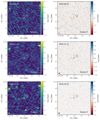 |
Fig. 1. Stokes-I (left) and Stokes-V (right) images of the area surrounding WX UMa. The images are formed from the entire 8 hour observation duration and entire 44 MHz bandwidth (120–167 MHz). The cross-hairs and circles show the proper-motion corrected position of WX UMa (GJ412 B) and GJ412 A, respectively, using the astrometric data from Gaia DR2 (Gaia Collaboration 2018). The flux densities of WX UMa and uncertainties are collated in Table 1. |
Details of LOFAR observations of WX UMa.
2.2. Spectro-temporal properties
The low frequency radio emission from WX UMa is broad-band and persistent. The emission persists for most of the 8 h observation block in each exposure, as seen in Fig. 2. The spectrum, shown in Fig. 3, is particularly interesting as it has a consistent shape across the observations: It is bright at the low-end of the observational band and rapidly declines within a few megahertz around ≈150 MHz to a level below our detection threshold. For instance, in the 2016 March 22 exposure (P167+42), for which we have the best Stokes-V sensitivity, the emission changes from ≈ − 1500 μJy at 124 MHz to being undetectable (below 3σ) in the three 7.8-MHz wide channels between ≈148 to ≈170 MHz, which have a root mean square (rms) noise of ≈140 μJy. This corresponds to a factor of ≈4 decline over a fractional bandwidth Δν/ν ≈ 0.15, where ν is the observing frequency. The decline in other epochs appears to be even more abrupt. However, the available signal-to-noise does not allow us to trace the spectral decline in finer channels. The small number of exposures (three) also does not allow a meaningful search for patterns in the location of the spectral turnover with an observation epoch.
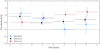 |
Fig. 2. Time resolved Stokes-I flux density of WX UMa averaged over the full 120–167 MHz band on the three independent exposures (see Table 1). The emission persists for most of the 8 h survey pointing duration. |
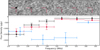 |
Fig. 3. Stokes-V spectrum of WX UMa in the three independent exposures from the LoTSS survey observations. The three sets of points show the spectrum for the three independent exposures. Upper limits correspond to 1σ. The greyscale images were made from the P167+42 exposure (see Table 1) over 8 h of synthesis and ≈7.8 MHz of bandwidth. The red cross-hairs mark the position of WX UMa. The source consistently shows a drop in flux density magnitude above ≈150 MHz in all epochs suggesting that this is an enduring property of the emitter. We made a 3.5-σ detection of WX UMa when averaging over the last three bands in the P167+42 observation, suggesting that the spectral evolution at these higher frequencies is a low plateau rather than a cut-off. |
We also averaged the images in the three 7.8-MHz channels of the P167+42 that yielded non-detections at the 3σ level. The averaged image, which is not shown here, revealed a faint 3.5σ source at the location of WX UMa. This suggests that the emission may settle into a low plateau as opposed to a total cut-off. Hence, despite the rapid decline, the emission does not appear to ‘turn off’ entirely at the high frequency end of our band. Further details on the radio data processing and extraction of dynamic spectra are given in Appendix A.
3. Discussion
The known properties of WX UMa which will aid in our interpretation of the radio emission are summarised in Table 2. Because the emission is persistent, we only consider cases where the emitting plasma is trapped within a closed magnetic geometry. This is because plasma that unbinds from the star is expected to expand on a timescale that is much shorter than the duration of our observations. For example, solar radio emission from plasma flowing along open field lines typically lasts from between seconds to minutes, as seen in solar Type-II and Type-III bursts (Wild & Smerd 1972).
Known properties of WX UMa from literature.
Magnetically trapped plasma in stellar coronae can emit via different mechanisms depending on the energy of the emitting electrons and the ambient magneto-ionic parameters (Dulk 1985). The high circular polarisation fraction rules out all known incoherent emission mechanisms. Coherent emission mechanisms that can generate up to 100% circularly polarised emission are fundamental plasma emission and fundamental and second harmonic cyclotron emission. While cyclotron emission occurs at the harmonics of the electron cyclotron frequency (Treumann 2006; Melrose & Dulk 1982), plasma emission in a magnetic trap is thought to occur at the harmonics of the upper hybrid frequency (Zaitsev & Stepanov 1983; Stepanov et al. 2001), which is the quadrature sum of the plasma and electron cyclotron frequencies. Both of these mechanisms can account for the long duration of the observed emission. Plasma emission persists for as long as the turbulent Langmuir wave spectrum that powers the emission is maintained. CMI from ultracool dwarfs is commonly seen to be pulsed at the rotation period due to beaming, but for conducive geometries, it can be visible at all rotation phases. CMI’s beaming geometry is discussed in more detail in Sect. 3.6 and Appendix C.
3.1. Emission site
The magnetic field of WX UMa is largely dipolar with a polar surface magnetic field strength of ≈4.5 kG (Morin et al. 2010). This yields a maximum cyclotron frequency at the surface of ≈12.6 GHz. Because a dipolar field evolves with radial distance R as R−3, fundamental cyclotron emission in the observed frequency band can only originate at a radial distance of ≈4.7R*, where R* is the stellar radius.
If the emission is due to the plasma mechanism, the emission site cannot be accurately pinpointed because the plasma density profile in WX UMa is not known a priori. However, a lower bound on the radial distance of the emission site can be placed based on the requirement for radiation escape. Escaping radiation in the presence of cyclotron damping is obtained when the ambient cyclotron frequency is sufficiently low: νc < 0.26νp (see Appendix B). Observable plasma emission at 120 MHz therefore requires the ambient magnetic field to be below ≈11 G. For a dipolar field that evolves with radial distance as R−3, this value can only be reached on WX UMa for R > 7.4 R*. We note that although there is a narrow window of low cyclotron opacity at small angles to the magnetic field for νc > 0.26νp (see Fig. A1 of Vedantham 2021), the bulk of the radiation is still absorbed since spontaneous plasma emission is quasi-isotropic.
3.2. Polarisation parity
The Zeeman doppler imaging (ZDI) maps of WX UMa show the star to have an intermediate inclination with a small magnetic obliquity and the south magnetic pole pointed towards us (i.e., field lines pointed towards the star; Morin et al. 2010). The observed radio emission is right-hand circularly polarised (see Appendix A.2 for details of sign convention). It is therefore in the o-mode if it originates in the polar regions, where the field points away from us, and x mode if it originates in the equatorial regions, where the field points towards us. Fundamental plasma emission is polarised in the o-mode, whereas cyclotron maser emission can be polarised in the x-mode or o-mode depending on the ambient plasma density (Dulk 1985; Vedantham 2021). Because WX UMa has a mostly axisymmetric dipolar field (Morin et al. 2010), we use cyclotron maser emission from Jupiter as a benchmark for our discussion for the possibility of cyclotron maser emission from WX UMa (Zarka 1998). Following this, the unstable electron distribution in a closed field region necessary to drive the cyclotron maser is expected to be situated close to the magnetic poles and, therefore, we only consider o-mode cyclotron emission. The o-mode cyclotron maser for a loss-cone distribution is expected to dominate for 0.1 ≲ νc/νp ≪ 1, with the x mode dominating at lower plasma densities (νc/νp ≲ 0.1) (Hewitt et al. 1982; Melrose & Dulk 1982). In summary, the observed polarity requires the emission to originate in the polar regions and be driven by either fundamental plasma emission, or o-mode cyclotron maser emission in which case νc/νp ≳ 0.1.
3.3. Extent of the closed field region
To recap, the two possibilities for the emission mechanism are the following: (a) plasma emission at a radial distance of > 7.4R* with an ambient density of ≈2 × 108 cm−3, and (b) a cyclotron maser at a radial distance of 4.7R* with an ambient density of ≳2 × 106 cm−3. Detailed MHD simulations are necessary to use these constraints to determine the size of the closed field region accurately, but we can place preliminary constraints with simplifying assumptions. We assume that the density has a hydrostatic profile with the inclusion of the centrifugal force (see Eq. (3) of Havnes & Goertz 1984). We then use the dipolar structure of the magnetic field and compute the equatorial distance at which the gas pressure (nkBT where T is the temperature, n is the number density, and kB is Boltzmann’s constant) is equal to the magnetic pressure. Beyond this radial distance, we assume that the gas forces open the field lines. So we identify this radial distance as the radius of the closed field region. Using this procedure and values relevant for WX UMa from Table 2, we find that the closed-open boundary occurs at radii of ≈10R* and 22R* for the case of fundamental plasma emission and cyclotron emission, respectively. Finally, the co-rotation radius, RC = (GM/Ω2)1/3 where G is the gravitational constant, Ω is the angular speed, and M is the stellar mass, is about 13.6R* for WX UMa. It is noteworthy that the corotation radius is comparable to the approximate open-closed boundary for the case of plasma emission.
3.4. Source of emitting electrons
With these considerations, it is still presently unclear what the source of the emitting electrons is in WX UMa, but we can draw analogies with two known systems. We first consider the solar paradigm for the case of plasma emission. In this case, the ultimate energy source is thought to be magnetic reconnection in coronal loops close to the surface (Priest & Forbes 2002). However, the brightness temperature arguments in Sect. 3.5 show that the solar paradigm can only apply to WX UMa if its entire coronal volume out to a radial distance of ≳7.4R* is filled with flaring loops which is unprecedented. We may alternatively adopt the Jovian paradigm, where cyclotron maser emission is emitted by suprathermal electrons (Dulk 1985) that are accelerated by the breakdown of co-rotation between the magnetic field and the magnetospheric plasma far from the planet’s surface, or by unipolar induction by its moons (Goldreich & Lynden-Bell 1969). A similar acceleration mechanism sited in the equatorial plasma sheet at a few tens of stellar radii may be responsible for WX UMa’s radio emission. Such an acceleration mechanism has also been suggested for magnetic chemically peculiar stars (Linsky et al. 1992). It it also noteworthy that both WX UMa and magnetic chemically peculiar stars have strong large-scale magnetic fields, hot X-ray coronae, and emit coherent circularly polarised emission (e.g., CU Vir, Trigilio et al. 2000).
3.5. Brightness temperature
The brightness temperature of the radio emitter assuming isotropic emission is Tb ≈ 1012.5x−2 K, where x is the radius of the emitter in units of the stellar radius. Theory allows the brightness temperature of cyclotron maser emission to be many orders of magnitude higher than this value (Treumann 2006; Melrose & Dulk 1982), and hence, the observed value can be readily accommodated. Fundamental plasma emission on the other hand cannot attain brightness temperatures ≫1012 K, especially at such low frequencies (Vedantham 2021). As shown in Sect. 3.1, the projected source radius for plasma emission is x ≈ 7.4, giving an observed brightness temperature of ∼1011 K. Although we note there is no precedence for plasma emission to be simultaneously occurring at this brightness throughout the corona (at x = 7.4 in this case), such a brightness temperature can be reached by plasma emission based on canonical theory if the plasma is highly turbulent (see Appendix A.2). Therefore, brightness temperature arguments do not provide a clear discriminant between the two plausible emission mechanisms.
3.6. Origin of the spectral evolution
Coherent stellar and planetary radio emission are known to display narrowband spectral features but their frequency centroid generally varies stochastically with time (see Litvinenko et al. 2009; Villadsen & Hallinan 2019, for examples)1. As such, the rapid spectral evolution from WX UMa is not unusual, but the persistent location of the spectral turnover is noteworthy. The persistence suggests that it encodes meaningful information on the nature and geometry of emission.
The expressions for the emissivity and absorption coefficients of various emission processes themselves vary smoothly, to polynomial order, with frequency (Zheleznyakov 1996). We must therefore seek an explanation for the rapid spectral evolution in terms of beaming, resonance conditions, or abrupt boundaries over which the plasma properties can change substantially. With this in mind, we consider three plausible explanations.
Beaming. If the emission is driven by the cyclotron maser mechanism, then a natural explanation for the cut-off would be due to beaming of the emission. Cyclotron maser emission is beamed into a hollow cone with a large opening angle, θ ≲ π/2, small thickness, Δθ ≪ θ, and whose axis is parallel to the ambient magnetic field. Radiation cones axes on a given field line make smaller angles with the magnetic axis at larger frequencies, as is illustrated in Fig. 4. Hence it is possible to construct geometries where the emission goes out of sight at higher frequencies. For example, in considering emission originating on field lines that intersect the equatorial plane at some radius L, if the magnetic field line makes a polar angle α(ν) at the point where emission at frequency ν originates, then the emission is visible to all observers within a magnetic co-latitude ‘visibility band’ that lies between θ − α(ν)−Δθ and θ + α(ν)+Δθ. If α(ν) evolves sufficiently rapidly with ν, then a spectral cut-off can be explained by beaming. It is possible that a spectral evolution could be observed due to the visibility-band edge moving over the line of sight to Earth within the observed frequency range. To address this possiblity, the function α(ν) can be computed for a given L, surface magnetic field strength, and dipolar geometry. For the case of LOFAR-band emission from WX UMa, the slope ∂α(ν)/∂ν varies between  and
and  as L is varied between 20R* and 6R* (further details are in the appendix). This corresponds to a shift in the visibility band by 1° and
  within a 20 MHz band within the observed frequency range. The angular shift is significantly smaller than the characteristic width of the emission cone’s surface, Δθ (Zarka 1998; Melrose & Dulk 1982), as well as other geometric parameters such as magnetic obliquity. Hence, an apparent cut-off due to beaming is possible but with a somewhat contrived geometric setup. Nevertheless, the beaming hypothesis can be tested by a search for a characteristic rotation and spectral modulation of the radio light curves at the rotation rate of WX UMa, which is an expected result of any magnetic obliquity in the system.
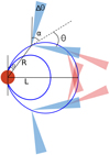 |
Fig. 4. Not-to-scale sketch showing the geometry of cyclotron maser emission on a single dipolar field line that lies in the plane of the page. The higher frequency emission cone (blue) is oriented at a smaller polar angle, α, when compared to the emission cone at a lower frequency (red). Here, L is the distance to the field line for a polar angle of 0°, R is the distance from the star’s centre to the emission cone along the field line, θ is the angle between the direction of emission and the interior wall of the cone, and Δθ is the angular width of the emission cone’s wall. The effects of α and θ on the emission frequency has been exaggerated here and is not to scale for the LOFAR frequency range. |
Resonant cyclotron absorption. If the emission is due to fundamental plasma emission, then the cut-off could be due to resonant cyclotron absorption of higher frequency emission that originates deeper in the corona. This is possible because the cyclotron frequency evolves with radial distance as R−3, whereas the plasma frequency can evolve much more gradually with radial distance, particularly if the density scale height is large. In such a situation, it is possible for the radiation escape condition to be satisfied at larger radii where lower frequency emission originates, but not at lower radii, where higher frequency emission originates, leading to a cut-off. Figure 5 shows plausible hydrostatic density profiles along different field lines, each with a different base density that leads to catastrophic cyclotron absorption within the LOFAR band. The density profiles all require that the base coronal density is restricted to a narrow range of values (about a 10% range) around 109.1 cm−3, which is comparable to the solar value. If this is the correct mechanism, then similar emission (long duration, highly polarised) must not be visible from WX UMa at frequencies above the LOFAR band and long-term monitoring should not show clear signs of rotation modulation in the LOFAR-band intensity. We note that WX UMa is detected between 2 and 4 GHz in the ongoing VLASS survey (Lacy et al. 2020) at a flux density of 1.3(1) mJy2. However, the VLASS survey observes with 3 minute exposures which is not long enough to associate the VLASS-detected emission with the long duration LOFAR-detected emission as opposed to a shorter duration burst.
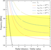 |
Fig. 5. Radial profile of the cyclotron frequency (solid black line) and the upper hybrid plasma frequency (coloured lines) for different base plasma density values given in units of cm−3. The plasma has been assumed to follow a hydrostatic density structure along any given field line while taking centrifugal force into account (Havnes & Goertz 1984, their Eq. (3)). The broken lines denote regions where cyclotron absorption precludes radiation escape. The yellow band shows the observed frequency range. |
Surface cut-off. The rapid spectral evolution can be explained if the bulk of the emission does not originate in WX UMa’s corona, but instead in the magnetosphere of a closeby (unresolved) sub-stellar companion and the cut-off frequency corresponds to a cyclotron frequency consistent with a surface magnetic field strength of ∼40 G, much in the same way Jovian cyclotron emission cuts off at around 40 MHz. This would be an unprecedented conclusion if true, as it would amount to a radio discovery of a sub-stellar companion (exoplanet or brown dwarf) around WX UMa. A prediction of this interpretation is periodic rotational modulation of the radio emission at a rate that does not match the known rotation rate of WX UMa. However, this property cannot be inferred from the current data since the emission has been detected in all three independent pointings.
In summary, we have identified three possible mechanisms to explain the rapid spectral evolution all of which can be tested with monitoring the LOFAR-band emission over several rotation cycles and with gigahertz frequency observations.
4. Summary and outlook
We have detected persistent, highly circularly polarised (≳70%) radio emission around 144 MHz from WX UMa. If the emission originates from WX UMa’s corona, there are two plausible emission mechanisms that can account for the radio emission: (a) plasma emission at the fundamental at a radial distance of ≳7.4R* where the ambient plasma density is ≈108.5 cm−3, and (b) o-mode cyclotron maser emission in which case the emission originates at a radial distance of ≈4.7R* where the ambient coronal density is 106.5 cm−3.
We expect our plasma density constraints to provide guidance to MHD simulations of the stellar wind of WX UMa. A simple balance between gas and magnetic pressure yield the radial extant of the closed field regions to be ≈10R* (plasma emission) and ≈22R* (cyclotron emission), respectively. Such radii are substantially larger than those that have been inferred from several MHD wind simulations of M-dwarfs (see for e.g., Vidotto et al. 2014), but they are comparable to recent simulation of M-dwarf winds with low mass-loss rates (Kavanagh et al. 2021). Interestingly, the closed–open field boundary in the equatorial plane for the plasma emission model is close to the co-rotation radius for WX UMa which is the anticipated extent of slingshot prominences (Jardine et al. 2020).
WX UMa’s radio spectrum shows a rapid decline within the observing band which could be a result of beaming of cyclotron emission or due to cyclotron absorption of plasma emission. Alternatively, the radio emission we observe might not have originated on WX UMa, but on a sub-stellar companion. All three possibilities can be tested with longer term multi-frequency monitoring of WX UMa’s radio emission.
A possible exception is AD Leo whose bursts observed by Villadsen & Hallinan (2019) show an apparent cut-off that is nearly consistent around 1.5 GHz.
Based on the VLASS ‘quick-look’ images. See https://science.nrao.edu/science/surveys/vlass
The LoTSS pipeline can be found at https://github.com/mhardcastle/ddf-pipeline
Acknowledgments
ID completed this work as part of the ASTRON summer student programme. JRC thanks the Nederlandse Organisatie voor Wetenschappelijk Onderzoek (NWO) for support via the Talent Programme Veni grant. AAV and TPR acknowledge funding from the European Research Council (ERC) under the European Union’s Horizon 2020 Research and Innovation Programme (grant agreements No 817540, ASTROFLOW and No 743029 EASY respectively). AD acknowledges support by the BMBF Verbundforschung under the grant 05A20STA. This paper is based on data obtained with the International LOFAR Telescope (obs. IDs 233996, 441476, 403966 and 403968) as part of the LoTSS survey. LOFAR is the Low Frequency Array designed and constructed by ASTRON. It has observing, data processing, and data storage facilities in several countries, that are owned by various parties (each with their own funding sources), and that are collectively operated by the ILT foundation under a joint scientific policy. The ILT resources have benefitted from the following recent major funding sources: CNRS-INSU, Observatoire de Paris and Université d’Orléans, France; BMBF, MIWF-NRW, MPG, Germany; Science Foundation Ireland (SFI), Department of Business, Enterprise and Innovation (DBEI), Ireland; NWO, The Netherlands; The Science and Technology Facilities Council, UK. This research made use of the Dutch national e-infrastructure with support of the SURF Cooperative (e-infra 180169) and the LOFAR e-infra group. The Jülich LOFAR Long Term Archive and the German LOFAR network are both coordinated and operated by the Jülich Supercomputing Centre (JSC), and computing resources on the supercomputer JUWELS at JSC were provided by the Gauss Centre for supercomputing e.V. (grant CHTB00) through the John von Neumann Institute for Computing (NIC). This research made use of the University of Hertfordshire high-performance computing facility and the LOFAR-UK computing facility located at the University of Hertfordshire and supported by STFC [ST/P000096/1], and of the Italian LOFAR IT computing infrastructure supported and operated by INAF, and by the Physics Department of Turin university (under an agreement with Consorzio Interuniversitario per la Fisica Spaziale) at the C3S Supercomputing Centre, Italy. The Jülich LOFAR Long Term Archive and the German LOFAR network are both coordinated and operated by the Jülich Supercomputing Centre (JSC), and computing resources on the supercomputer JUWELS at JSC were provided by the Gauss Centre for Supercomputing e.V. (grant CHTB00) through the John von Neumann Institute for Computing (NIC).
References
- Alonso-Floriano, F. J., Morales, J. C., Caballero, J. A., et al. 2015, A&A, 577, A128 [NASA ADS] [CrossRef] [EDP Sciences] [Google Scholar]
- Callingham, J. R., Vedantham, H. K., Pope, B. J. S., Shimwell, T. W., & LoTSS Team 2019, Res. Notes Am. Astron. Soc., 3, 37 [Google Scholar]
- Callingham, J. R., Pope, B. J. S., Feinstein, A. D., et al. 2021a, A&A, 648, A13 [EDP Sciences] [Google Scholar]
- Callingham, J. R., Vedantham, H. K., Shimwell, T. W., & Pope, B. J. S. 2021b, Nat. Astron., submitted [Google Scholar]
- Cohen, O., Drake, J. J., Glocer, A., et al. 2014, ApJ, 790, 57 [NASA ADS] [CrossRef] [Google Scholar]
- Collier Cameron, A., & Robinson, R. D. 1989, MNRAS, 238, 657 [NASA ADS] [CrossRef] [Google Scholar]
- Dressing, C. D., & Charbonneau, D. 2015, ApJ, 807, 45 [NASA ADS] [CrossRef] [Google Scholar]
- Dulk, G. A. 1985, ARA&A, 23, 169 [NASA ADS] [CrossRef] [Google Scholar]
- Gaia Collaboration (Brown, A. G. A., et al.) 2018, A&A, 616, A1 [NASA ADS] [CrossRef] [EDP Sciences] [Google Scholar]
- Garraffo, C., Drake, J. J., Cohen, O., Alvarado-Gómez, J. D., & Moschou, S. P. 2017, ApJ, 843, L33 [NASA ADS] [CrossRef] [Google Scholar]
- Gillon, M., Triaud, A. H. M. J., Demory, B.-O., et al. 2017, Nature, 542, 456 [Google Scholar]
- Goldreich, P., & Lynden-Bell, D. 1969, ApJ, 156, 59 [NASA ADS] [CrossRef] [Google Scholar]
- Güdel, M. 2002, ARA&A, 40, 217 [NASA ADS] [CrossRef] [Google Scholar]
- Hancock, P. J., Murphy, T., Gaensler, B. M., Hopkins, A., & Curran, J. R. 2012, MNRAS, 422, 1812 [NASA ADS] [CrossRef] [Google Scholar]
- Havnes, O., & Goertz, C. K. 1984, A&A, 138, 421 [NASA ADS] [Google Scholar]
- Hewitt, R. G., Melrose, D. B., & Ronnmark, K. G. 1982, Aust. J. Phys., 35, 447 [CrossRef] [Google Scholar]
- Jardine, M., Collier Cameron, A., Donati, J. F., & Hussain, G. A. J. 2020, MNRAS, 491, 4076 [Google Scholar]
- Johnstone, C. P., & Güdel, M. 2015, A&A, 578, A129 [NASA ADS] [CrossRef] [EDP Sciences] [Google Scholar]
- Kavanagh, R. D., Vidotto, A. A., Klein, B., et al. 2021, MNRAS, 504, 1511 [Google Scholar]
- Kopparapu, R. K., Ramirez, R., Kasting, J. F., et al. 2013, ApJ, 765, 131 [Google Scholar]
- Lacy, M., Baum, S. A., Chandler, C. J., et al. 2020, PASP, 132, 035001 [CrossRef] [Google Scholar]
- Linsky, J. L., Drake, S. A., & Bastian, T. S. 1992, ApJ, 393, 341 [NASA ADS] [CrossRef] [Google Scholar]
- Litvinenko, G. V., Lecacheux, A., Rucker, H. O., et al. 2009, A&A, 493, 651 [NASA ADS] [CrossRef] [EDP Sciences] [Google Scholar]
- Lynch, C. R., Lenc, E., Kaplan, D. L., Murphy, T., & Anderson, G. E. 2017, ApJ, 836, L30 [NASA ADS] [CrossRef] [Google Scholar]
- Melrose, D. B., & Dulk, G. A. 1982, ApJ, 259, 844 [NASA ADS] [CrossRef] [Google Scholar]
- Morin, J., Donati, J. F., Petit, P., et al. 2010, MNRAS, 407, 2269 [NASA ADS] [CrossRef] [MathSciNet] [Google Scholar]
- Newton, E. R., Irwin, J., Charbonneau, D., et al. 2017, ApJ, 834, 85 [NASA ADS] [CrossRef] [Google Scholar]
- Pneuman, G. W. 1968, Sol. Phys., 3, 578 [Google Scholar]
- Priest, E. R., & Forbes, T. G. 2002, A&ARv, 10, 313 [NASA ADS] [CrossRef] [Google Scholar]
- Shimwell, T. W., Röttgering, H. J. A., Best, P. N., et al. 2017, A&A, 598, A104 [NASA ADS] [CrossRef] [EDP Sciences] [Google Scholar]
- Shimwell, T. W., Tasse, C., Hardcastle, M. J., et al. 2019, A&A, 622, A1 [NASA ADS] [CrossRef] [EDP Sciences] [Google Scholar]
- Stepanov, A. V., Kliem, B., Zaitsev, V. V., et al. 2001, A&A, 374, 1072 [NASA ADS] [CrossRef] [EDP Sciences] [Google Scholar]
- Tasse, C., Shimwell, T., Hardcastle, M. J., et al. 2021, A&A, 648, A1 [EDP Sciences] [Google Scholar]
- Treumann, R. A. 2006, A&ARv, 13, 229 [NASA ADS] [CrossRef] [Google Scholar]
- Trigilio, C., Leto, P., Leone, F., Umana, G., & Buemi, C. 2000, A&A, 362, 281 [Google Scholar]
- van Haarlem, M. P., Wise, M. W., Gunst, A. W., et al. 2013, A&A, 556, A2 [NASA ADS] [CrossRef] [EDP Sciences] [Google Scholar]
- van Straten, W., Manchester, R. N., Johnston, S., & Reynolds, J. E. 2010, PASA, 27, 104 [NASA ADS] [Google Scholar]
- van Weeren, R. J., Shimwell, T. W., Botteon, A., et al. 2021, A&A, in press, https://doi.org/10.1051/0004-6361/202039826 [Google Scholar]
- Vedantham, H. K. 2021, MNRAS, 500, 3898 [Google Scholar]
- Vedantham, H. K., Callingham, J. R., Shimwell, T. W., et al. 2020a, Nat. Astron., 4, 577 [CrossRef] [Google Scholar]
- Vedantham, H. K., Callingham, J. R., Shimwell, T. W., et al. 2020b, ApJ, 903, L33 [Google Scholar]
- Vidotto, A. A. 2021, Liv. Rev. Sol. Phys., 18, 3 [Google Scholar]
- Vidotto, A. A., Jardine, M., Morin, J., et al. 2013, A&A, 557, A67 [NASA ADS] [CrossRef] [EDP Sciences] [Google Scholar]
- Vidotto, A. A., Jardine, M., Morin, J., et al. 2014, MNRAS, 438, 1162 [NASA ADS] [CrossRef] [Google Scholar]
- Villadsen, J., & Hallinan, G. 2019, ApJ, 871, 214 [NASA ADS] [CrossRef] [Google Scholar]
- Wild, J. P., & Smerd, S. F. 1972, ARA&A, 10, 159 [NASA ADS] [CrossRef] [Google Scholar]
- Zaitsev, V. V., & Stepanov, A. V. 1983, Sol. Phys., 88, 297 [NASA ADS] [CrossRef] [Google Scholar]
- Zarka, P. 1998, J. Geophys. Res., 103, 20159 [NASA ADS] [CrossRef] [Google Scholar]
- Zheleznyakov, V. V. 1996, Radiation in Astrophysical Plasmas (Kluwer academic publishers), 204 [CrossRef] [Google Scholar]
Appendix A: Radio data processing
A.1. Data reduction pipeline
The data were processed with the usual LoTSS pipeline3 (Shimwell et al. 2017, 2019), which is described in Tasse et al. (2021). We then performed an additional round of self-calibration in the direction of WX UMa with a procedure described in van Weeren et al. (2021) and also employed in Vedantham et al. (2020a). After calibration, the measurement set was further processed to make source extraction easier for producing light curves and spectra. WX UMa was removed from the mask image which was then used to produce a model file using WSClean. WX UMa was also removed from these model images so that it would not be removed during the subtraction of other sources. The subtracted model image was then used with WSClean again to predict visibilities which were recorded in a new modelled data column in the measurement set. The modelled data was subtracted from the real data column and recorded in a new column; this served to remove all other bright sources from the region besides WX UMa. Finally, DPPP was used to phaseshift the measurement sets to be centred on WX UMa, using the subtracted data as the new real data.
After extra sources were removed from the field and the set was phaseshifted, frequency and time slices for Stokes-I and V were produced via WSClean. Because the signal-to-noise ratio of the observation was not large enough to produce a full dynamic spectrum, the frequency slices were averaged over all time and the time slices were averaged over the first 40 channels (120 to 135.83 MHz, ≈16 MHz bandwidth) where WX UMa is the brightest. The background and noise estimation (BANE) tool in Aegean (Hancock et al. 2012) was used with each image to produce rms and background images. Aegean was run with a 4σ seedclip to avoid identifying extraneous sources. The flux density for WX UMa for a particular image was assigned from the peak flux found by Aegean if a source was found in the expected location of WX UMa, and the rms noise was retrieved from the rms image produced by BANE. For images where no 4σ source was found at the star’s coordinates, a priorized fitting was applied using the catalogue from the image with the most significant detection in order to extract ≈3σ detections at the expected position of WX UMa. The images were also inspected by eye to make sure the results of Aegean were consistent with the images. The temporal evolution of WX UMa’s radio flux is shown in Fig. 2 and its spectral evolution is shown in Fig. 3. We note that some of the images of the light curve estimation have non-Gaussian noise due to residual sidelobe noise (from poorer uv coverage) and low-level calibration errors.
A.2. Stokes-V sign convention
There are two commonly used Stokes-V sign conventions in literature. The pulsar literature typically follows the convention V = LCP − RCP, whereas the IAU convention is V = RCP − LCP (van Straten et al. 2010). To check the convention applicable to the LoTSS images, we compared the sign of Stokes-V of several pulsar detections to that in the literature and found that the LoTSS survey data products follow the same convention as the one in pulsar literature (Callingham et al. 2021b). Hence, WX UMa is radiating RCP radiation, which means that the electric field vector rotates anticlockwise as a function of time to an observer looking at incoming radiation.
Appendix B: Emission mechanism
B.1. Brightness temperature of plasma emission
In Fig. B.1, we computed the brightness temperature of plasma emission using the expressions of Stepanov et al. (2001, specifically, their Eq. (15)). In doing so, we assumed a peak turbulence level of w = 10−5 and to compute the plasma temperature, we used the empirical relationship of Johnstone & Güdel (2015) and the observed X-ray luminosity (Table 2).
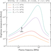 |
Fig. B.1. Brightness temperature of plasma emission computed for parameters relevant for WX UMa (annotated in the figure). The black bar is the measured value based on the radiation escape conditions and the assumption that the entire projected coronal surface is radiating. |
B.2. Escape of plasma emission
Fundamental plasma emission is excited at the upper-hybrid frequency:  where νp and νc are the plasma and cyclotron frequencies, respectively. We note that the upper-hybrid frequency is always larger than the cyclotron frequency. The cyclotron absorption optical depth for o-mode radiation propagating at an angle θ to the magnetic field may be approximated by
 (B.1)
(B.1)
where the integer s = ν/νc > 1 is the cyclotron harmonic number, T is the coronal temperature, me is the electron mass, c is the speed of light, kB is Boltzmann’s constant, and LB is the magnetic scale length which we take to be R*. For the parameters of interest: T ∼ 106.7 K, LB ∼ 1010 cm, and the optical depth is safely below unity for only s ≥ 4. Hence, the radiation escape condition is  , which gives νc < 0.26νp.
Appendix C: Spectral evolution of the emission cone
In considering a single dipolar field line which intersects the equatorial plane at radial distance L, the radial distance and polar angle, θ′, along the field line are related via L = Rsin2θ′. The polar inclination angle of the field lines, α, is given by cos α = (3cos2θ′−1)(1 + 3cos2θ′)−1/2. The magnetic field strength, and cyclotron frequency, vary continuously along the field line according to  , where ν0 is the peak cyclotron frequency at θ′ = 0, R = R*. With the above relationships, we predicted the inclination of the emission cone axis for various L-shells at a range of cyclotron frequencies (see Fig. C.1). The numerically computed slope of the α versus ν lines at 140 MHz vary between ∂α/∂ν ≈ 0.2 ° /MHz and ∂α/∂ν ≈ 0.8 ° /MHz as L is varied between 6 and 20. The magnitude of the slope decreases for larger L and must asymptote to zero as L tends to infinity.
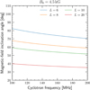 |
Fig. C.1. Polar angle of the magnetic field at the site of emission (y-axis) versus frequency of emission (x-axis) for different field lines specified by the radial distance at which they intersect the equatorial plane. |
All Tables
All Figures
|
Fig. 1. Stokes-I (left) and Stokes-V (right) images of the area surrounding WX UMa. The images are formed from the entire 8 hour observation duration and entire 44 MHz bandwidth (120–167 MHz). The cross-hairs and circles show the proper-motion corrected position of WX UMa (GJ412 B) and GJ412 A, respectively, using the astrometric data from Gaia DR2 (Gaia Collaboration 2018). The flux densities of WX UMa and uncertainties are collated in Table 1. |
| In the text | |
|
Fig. 2. Time resolved Stokes-I flux density of WX UMa averaged over the full 120–167 MHz band on the three independent exposures (see Table 1). The emission persists for most of the 8 h survey pointing duration. |
| In the text | |
|
Fig. 3. Stokes-V spectrum of WX UMa in the three independent exposures from the LoTSS survey observations. The three sets of points show the spectrum for the three independent exposures. Upper limits correspond to 1σ. The greyscale images were made from the P167+42 exposure (see Table 1) over 8 h of synthesis and ≈7.8 MHz of bandwidth. The red cross-hairs mark the position of WX UMa. The source consistently shows a drop in flux density magnitude above ≈150 MHz in all epochs suggesting that this is an enduring property of the emitter. We made a 3.5-σ detection of WX UMa when averaging over the last three bands in the P167+42 observation, suggesting that the spectral evolution at these higher frequencies is a low plateau rather than a cut-off. |
| In the text | |
|
Fig. 4. Not-to-scale sketch showing the geometry of cyclotron maser emission on a single dipolar field line that lies in the plane of the page. The higher frequency emission cone (blue) is oriented at a smaller polar angle, α, when compared to the emission cone at a lower frequency (red). Here, L is the distance to the field line for a polar angle of 0°, R is the distance from the star’s centre to the emission cone along the field line, θ is the angle between the direction of emission and the interior wall of the cone, and Δθ is the angular width of the emission cone’s wall. The effects of α and θ on the emission frequency has been exaggerated here and is not to scale for the LOFAR frequency range. |
| In the text | |
|
Fig. 5. Radial profile of the cyclotron frequency (solid black line) and the upper hybrid plasma frequency (coloured lines) for different base plasma density values given in units of cm−3. The plasma has been assumed to follow a hydrostatic density structure along any given field line while taking centrifugal force into account (Havnes & Goertz 1984, their Eq. (3)). The broken lines denote regions where cyclotron absorption precludes radiation escape. The yellow band shows the observed frequency range. |
| In the text | |
|
Fig. B.1. Brightness temperature of plasma emission computed for parameters relevant for WX UMa (annotated in the figure). The black bar is the measured value based on the radiation escape conditions and the assumption that the entire projected coronal surface is radiating. |
| In the text | |
|
Fig. C.1. Polar angle of the magnetic field at the site of emission (y-axis) versus frequency of emission (x-axis) for different field lines specified by the radial distance at which they intersect the equatorial plane. |
| In the text | |
Current usage metrics show cumulative count of Article Views (full-text article views including HTML views, PDF and ePub downloads, according to the available data) and Abstracts Views on Vision4Press platform.
Data correspond to usage on the plateform after 2015. The current usage metrics is available 48-96 hours after online publication and is updated daily on week days.
Initial download of the metrics may take a while.