| Issue |
A&A
Volume 650, June 2021
|
|
|---|---|---|
| Article Number | A89 | |
| Number of page(s) | 11 | |
| Section | Planets and planetary systems | |
| DOI | https://doi.org/10.1051/0004-6361/202140758 | |
| Published online | 09 June 2021 | |
Three microlensing planets with no caustic-crossing features
1
Department of Physics, Chungbuk National University,
Cheongju
28644,
Republic of Korea
e-mail: This email address is being protected from spambots. You need JavaScript enabled to view it.
2
Astronomical Observatory, University of Warsaw,
Al. Ujazdowskie 4,
00-478
Warszawa, Poland
3
Korea Astronomy and Space Science Institute,
Daejon
34055, Republic of Korea
4
Department of Physics and Astronomy, University of Canterbury,
Private Bag 4800,
Christchurch
8020, New Zealand
5
Korea University of Science and Technology,
217 Gajeong-ro,
Yuseong-gu, Daejeon,
34113, Republic of Korea
6
Max Planck Institute for Astronomy,
Königstuhl 17,
69117
Heidelberg, Germany
7
Department of Astronomy, The Ohio State University,
140 W. 18th Ave.,
Columbus,
OH
43210, USA
8
Department of Particle Physics and Astrophysics, Weizmann Institute of Science,
Rehovot
76100, Israel
9
Center for Astrophysics, Harvard & Smithsonian 60 Garden St.,
Cambridge,
MA
02138, USA
10
Department of Astronomy, Tsinghua University,
Beijing
100084,
PR China
11
School of Space Research, Kyung Hee University,
Yongin,
Kyeonggi
17104, Republic of Korea
12
Division of Physics, Mathematics, and Astronomy, California Institute of Technology,
Pasadena,
CA
91125, USA
13
Department of Physics, University of Warwick,
Gibbet Hill Road,
Coventry,
CV4 7AL, UK
Received:
9
March
2021
Accepted:
13
April
2021
Abstract
Aims. We search for microlensing planets with signals exhibiting no caustic-crossing features, considering the possibility that such signals may be missed due to their weak and featureless nature.
Methods. For this purpose, we reexamine the lensing events found by the KMTNet survey before the 2019 season. From this investigation, we find two new planetary lensing events, KMT-2018-BLG-1976 and KMT-2018-BLG-1996. We also present the analysis of the planetary event OGLE-2019-BLG-0954, for which the planetary signal was known but no detailed analysis had previously been presented. We identify the genuineness of the planetary signals by checking various interpretations that can generate short-term anomalies in lensing light curves.
Results. From Bayesian analyses conducted with the constraint from available observables, we find that the host and planet masses are (M1, M2) ~ (0.65 M⊙, 2 MJ) for KMT-2018-BLG-1976L, ~(0.69 M⊙, 1 MJ) for KMT-2018-BLG-1996L, and ~(0.80 M⊙, 14 MJ) for OGLE-2019-BLG-0954L. The estimated distance to OGLE-2019-BLG-0954L, 3.63−1.64+1.22 kpc, indicates that it is located in the disk, and the brightness expected from the mass and distance matches the brightness of the blend well, indicating that the lens accounts for most of the blended flux. The lens of OGLE-2019-BLG-0954 may be resolved from the source by conducting high-resolution follow-up observations in and after 2024.
Key words: gravitational lensing: micro / planets and satellites: detection
© ESO 2021
1 Introduction
The microlensing signal of a planet is characterized by a short-term anomaly appearing on the smooth single-lens single-source (1L1S) light curve produced by the host of the planet (Mao & Paczyński 1991; Gould & Loeb 1992). The signal is produced because the planet induces caustics, denoting the source positions at which the lensing magnification of a point source becomes infinite. The majority of microlensing planets reported so far1 have been detected through caustic-crossing features, which are produced by the passage of a source over the planet-induced caustic. However, planetary signals can still be generated without a caustic crossing of the source. This is because the magnification excess induced by a planet extends to a considerable region beyond the caustic, and thus a planetary signal can be produced by the approach of the source to the caustic, rather than a crossing: This is the “non-caustic-crossing channel” (e.g., OGLE-2016-BLG-1067Lb; Calchi Novati et al. 2019). The non-caustic-crossing channel is important because its cross section to a planetary signal is substantially larger than the caustic size. Zhu et al. (2014) estimated that about half of all detectable events from a high-cadence lensing survey should lack caustic features.
Despite the large cross section, planets detected through the non-caustic-crossing channel comprise a minor fraction of all reported microlensing planets. The relative rarity of planets discovered through the non-caustic-crossing channel is mostly attributed to the difficulty of detecting planetary signals. Two factors contribute to this difficulty. First, planetary signals with no caustic-crossing features are likely to be weak. Due to the nature of the caustic, the planetary signal produced by the caustic crossing is usually strong, although the strength varies depending on the source size. In contrast, the strength of the non-caustic-crossing signal is much weaker because the source flux does not go through a great magnification induced by the caustic. For the same reason, planetary signals produced by caustic crossings can be missed if the caustic-crossing features are not covered. Second, planetary signals produced by the non-caustic-crossing channel tend to be featureless. Caustic-crossing planetary signals usually exhibit characteristic features, such as the caustic-crossing spikes and the U-shape trough between the spikes, and this helps make the signal easy to notice. On the contrary, non-caustic-crossing signals, in most cases, do not exhibit a noticeable feature that identifies the planetary origin of the signal.
Another reason for the lack of planet reports detected through the non-caustic-crossing channel is rooted in the difficulty of finding scientific issues that might draw attention. In most cases, important scientific issues for discovered planets are drawn from their physical parameters, such as mass and distance. For microlensing planets, these parameters can be determined by measuring extra observables in addition to the basic observable of the lensing event timescale, tE. These extra observables are the microlens parallax, πE, and the angular Einstein radius, θE. The microlens parallax is measurable for long timescale events, in which the lensing light curves exhibit deviations from a symmetric form due to the orbital motion of Earth around the Sun (Gould 1992). The angular Einstein radius is measurable for caustic-crossing planetary events, in which the light curve during the caustic crossing exhibits deviations from a point-source form due to finite-source effects. For planets detected through the non-caustic-crossing channel, however, it is difficult to measure θE because the lensing light curve is not subject to finite-source effects. This makes it difficult to uniquely measure the physical parameters of the detected planetary system. For this reason, some planetary lensing events are left without detailed analyses even after planetary signals are noticed. Nevertheless, it is important to report all detected planets for the construction of a complete planet sample, from which the planet frequency and demographic properties are deduced.
In this paper, we report the third result from the project, which was conducted by reinvestigating the data collected by the Korea Microlensing Telescope Network (KMTNet; Kim et al. 2016) survey before the 2019 season with the aim of finding unrecognized planetary signals. In the first part of the project, Han et al. (2020b) reexamined lensing events associated with faint source stars, considering the possibility that planetary signals in these events might be missed due to the large photometric uncertainty. From this work, they reported four unnoticed or unpublished microlensing planets: KMT-2016-BLG-2364Lb, KMT-2016-BLG-2397Lb, OGLE-2017-BLG-0604Lb, and OGLE-2017-BLG-1375Lb. In the second part of the project, Han et al. (2021) reported a super-Earth planet orbiting a very low-mass star, KMT-2018-BLG-1025Lb, found from the systematic inspection of high-magnification microlensing events in the previous data. The result that we report in this paper comes from the third part of the project. In this work, we reinvestigate lensing events to search for microlensing planets with no caustic-crossing features. From this investigation, we find two planetary lensing events, KMT-2018-BLG-1976 and KMT-2018-BLG-1996, for which the planetary signals were not previously noticed. We also present the analysis of the planetary event OGLE-2019-BLG-0954, for which the planetary signal was known but no detailed analysis had been presented.
For the presentation of the analysis, we organize the paper as follows. In Sect. 2, we describe the observations of the analyzed events and the data acquired from the observations. In Sect. 3, we describe details of the modeling conducted to explain the observed anomalies in the lensing light curves. In Sect. 4, we characterize the source stars of the events and test the possibility of constraining θE. In Sect. 5, we estimate the physical lens parameters using the available observables. We discuss some of the implications of these results in Sect. 6 and conclude in Sect. 7.
2 Observation and data
The three planetary lensing events KMT-2018-BLG-1976, KMT-2018-BLG-1996, and OGLE-2019-BLG-0954 commonly occurred on stars located toward the Galactic bulge field. The equatorial and galactic coordinates of the individual events are listed in Table 1.
The events KMT-2018-BLG-1976 and KMT-2018-BLG-1996 were found from the post-season searches for lensing events in the data collected during the 2018 season by the KMTNet survey using the Event Finder System algorithm (Kim et al. 2018). While KMT-2018-BLG-1976 and KMT-2018-BLG-1996 were found solely by the KMTNet survey, the event OGLE-2019-BLG-0954/KMT-2019-BLG-3289 was found by two surveys, first by the Optical Gravitational Lensing Experiment (OGLE; Udalski et al. 2015) survey and later by the KMTNet survey. Hereafter, we designate this event as OGLE-2019-BLG-0954 according to the chronological order of the discoveries. The observations by the KMTNet survey were conducted using the three identical telescopes that are globally located on three continents: the Siding Spring Observatory in Australia (KMTA), the Cerro Tololo Interamerican Observatoryin Chile (KMTC), and the South African Astronomical Observatory in South Africa (KMTS). The aperture of each KMTNet telescope is 1.6 m, and the field of view of the camera mounted on the telescope is 4 deg2. The observations by the OGLE survey were done using the 1.3 m telescope located at the Las Campanas Observatory in Chile. The OGLE telescope is equipped with a camera yielding a 1.4 deg2 field of view.
For both surveys, the images of the source stars were obtained mainly in the I band, and a fraction of images were acquired in the V band for the source color measurement. We describe the detailed procedure of the source color measurements in Sect. 4. The observational cadence varies depending on the events and surveys. The events KMT-2018-BLG-1976 and KMT-2018-BLG-1996 were located in the KMT37 and KMT38 fields, respectively, and both fields were observed with a 2.5 h cadence. The event OGLE-2019-BLG-0954 was located in the OGLE501 and KMT02+KMT42 fields, which were observed with cadences of 1 h and of 15 min, respectively. We note that KMT-2018-BLG-1976 is not in the OGLE footprint and that KMT-2018-BLG-1996 lies in the OGLE field BLG642, which was not observed for microlensing purposes after 2016.
Reduction of the data and photometry of the events was carried out using the software pipelines developed by the individual survey groups: Albrow et al. (2009) for KMTNet and Woźniak (2000) for OGLE. Both of these photometry codes are based on the difference imaging technique (Tomaney & Crotts 1996; Alard & Lupton 1998), which is optimized for dense-field photometry. Following the routine described in Yee et al. (2012), we readjusted the error bars of the data estimated from the automatized pipelines, first to account for the scatter of the data and second to make the χ2 per degree of freedom for each data set become unity.
Coordinates and fields.
3 Analyses
The light curves of the three events analyzed in this work commonly exhibit weak anomalies with short durations. In order to reveal the origins of the anomalies, we tested three models under the 1L1S, 2L1S, and 1L2S interpretations. The 2L1S modeling was done under the interpretation that the lens is a binary object, while the 1L2S modeling was conducted under the interpretation that the source is a binary. The 2L1S modeling was done because a short-term anomaly can be produced by a planetary companion to the lens. The 1L2S model was tested because a subset of 1L2S events can produce short anomalies that mimic planetary signals (Gaudi 1998).
A lensing light curve is described by different sets of parameters depending on the interpretation. A 1L1S lensing light curve is described by three parameters, (t0, u0, tE), which denote the peak time at the closest lens-source approach, the lens-source separation at t0 (impact parameter), and the event timescale, respectively. The event timescale is defined as the time required for the source to cross the angular Einstein radius of the lens, that is, tE = θE∕μ, where μ denotes the relative lens-source proper motion. Modeling a 2L1S light curve requires additional parameters to describe the binarity of the lens. These extra parameters are (s, q, α), which indicate, respectively: the projected binary lens separation (scaled to θE); the mass ratio between the lens components, M1 and M2 ; and the angle between the source trajectory and the M1 –M2 axis (source trajectory angle). For the description of the lensing light curve with an anomaly caused by a caustic crossing, during which the light curve is affected by finite-source effects, it is required to include an extra parameter, ρ, which is defined as the ratio of the angular source radius, θ*, to the angular Einstein radius, that is, ρ = θ*∕θE (normalized source radius). Describing the source binarity also requires the inclusion of additional parameters, (t0,2, u0,2, ρ2, qF), the first two of which are the closest time and separation between the second source and the lens, the third is the normalized source radius of the second source, and the last denotes the flux ratio between the source stars. In the following subsections, we present details of the analyses conducted for the individual events.
3.1 KMT-2018-BLG-1976
Figure 1 shows the lensing light curve of the event KMT-2018-BLG-1976. It shows that the lensing-induced magnification of the source flux started during the time gap between the end of the 2017 season and the beginning of the 2018 season. The light curve reached its peak on March 5, 2018, HJD′≡HJD − 2 450 000 ~ 8183, at which point the source became brighter by ΔI ~ 1.9 magnitude than the baseline magnitude of Ibase = 18.02, according to the KMTNet scale, and then gradually returned to its baseline. At first glance, the light curve appears to be that of a 1L1S event. The 1L1S modeling yields the lensing parameters of (u0, tE) ~ (0.14, 42.3 days), indicating that the source flux was magnified by ![Mathematical equation: $A_{\textrm{peak}}\,{=}\,(u_0+2)/[u_0(u_0^2+4)^{1/2}]\sim 7.2$](/articles/aa/full_html/2021/06/aa40758-21/aa40758-21-eq2.png) at the peak. The 1L1S model curve is drawn over the data points in Fig. 1, and the full lensing parameters and their uncertainties are listed in Table 2. However, a close inspection reveals that the light curve exhibits an anomaly that appears around the peak. In Fig. 2, we present the enlarged view of the peak region along with the residuals from the 1L1S model. The anomaly, which lasted for about 6 days during the period of 8184 ≲HJD′≲ 8190, shows negative deviations in most of the anomaly region, but it exhibits a slight positive deviation at the beginning of the anomaly. Although the deviation of the anomaly is small, ≲0.1 mag, we consider the anomaly to be significant because the data obtained by the different telescopes delineate a consistent pattern of deviation.
at the peak. The 1L1S model curve is drawn over the data points in Fig. 1, and the full lensing parameters and their uncertainties are listed in Table 2. However, a close inspection reveals that the light curve exhibits an anomaly that appears around the peak. In Fig. 2, we present the enlarged view of the peak region along with the residuals from the 1L1S model. The anomaly, which lasted for about 6 days during the period of 8184 ≲HJD′≲ 8190, shows negative deviations in most of the anomaly region, but it exhibits a slight positive deviation at the beginning of the anomaly. Although the deviation of the anomaly is small, ≲0.1 mag, we consider the anomaly to be significant because the data obtained by the different telescopes delineate a consistent pattern of deviation.
In order to explain the anomaly, we first tested a 1L2S model. The 1L2S modeling was done with the initial parameters of (t0, u0, tE) obtained from the 1L1S modeling, and the initial values of the parameters related to the second source, (t0,2, u0,2.ρ2, qF), were assigned considering the magnitude and the location of the anomaly in the lensing light curve. This modeling yields the lensing parameters of (u0, u0,2, qF) ~ (0.12, 0.10, 0.07), indicating that the second source, S2, with a flux of about 7% of the flux from the primary source, S1, approaches closer to the lens than S1 does. The full lensing parameters and their 1L2S model uncertainties are listed in Table 2, and the model curve and the residuals are shown in Fig. 2. The introduction of an extra source improves the fit by Δχ2 ~ 17.1 with respect to the 1L1S model, reducing the depth of the negative deviations. However, the model still leaves subtle but noticeable deviations, indicating that a different interpretation is needed.
We then tested a 2L1S model. The 2L1S modeling was conducted in two steps. In the first step, we conducted a grid search for the binary lens parameters (s, q), while the other parameters were searched for based on the downhill χ2 minimization approach using the Markov chain Monte Carlo (MCMC) algorithm. This step enabled us to find local solutions that are subject to various types of degeneracy. In the second step, we inspected the local solutions in the s–q parameter space and then refined them by allowing all parameters (including s and q) to vary. We list the best-fit lensing parameters of the 2L1S model in Table 2.
We identified two 2L1S solutions, one with s > 1 and the other with s < 1. Very often, when two such solutions are found, they are identified as, respectively, the “wide” and “close” degenerate solutions that Griest & Safizadeh (1998) and Dominik (1999) identified for central caustics. In the present case, however, this is not correct. This is actually the “outer–inner” degeneracy for planetary caustics that was identified by Gaudi & Gould (1997). From Fig. 3, one can see that, in both cases, the dip is produced by the source crossing the long trough that extends along the planet–host axis on the opposite side of the planet. In the close (inner) solution, there is a separate set of planetary caustics, and the source passes “inside” these (i.e., between these caustics and the central caustic). In the wide (outer) solution, the planetary and central caustics have merged into a single, so-called resonant caustic. However, it is still the case that there is a long trough extending from the “back end” of the resonant caustic that retains substantial structure from the previously separate planetary caustics. The source passes “outside” the tips of these structures.
Herrera-Martín et al. (2020) were the first to recognize that this pair of caustic morphologies is the inner–outer degeneracy. Indeed, the light curve of OGLE-2018-BLG-0677, which they analyzed, looks remarkably similar to that of KMT-2018-BLG-1976, except that the duration of the dip is much shorter. Closely related to this fact, the difference in the two values of s is much smaller, Δs = (sw − sc)∕2 = 0.03 (versus 0.26 in the present case), and both values of s were less than 1.0. Here, sw and sc denote the binary separations of the wide and close solutions, respectively. The opposite of the present case was seen in OGLE-2016-BLG-1195 (Bond et al. 2017; Shvartzvald et al. 2017), in which a non-caustic “bump” was observed rather than a “dip,” which yielded an inner–outer degeneracy but one offset from the major-image planetary caustic (rather than the minor-image caustic as for KMT-2018-BLG-1976). In that case as well, sc < 1 and sw > 1. However, Δs = 0.05, a factor of five smaller than in the present case.
Yee et al. (2021) have conjectured that there is a continuous transition between the inner–outer planetary-caustic degeneracy of Gaudi & Gould (1997) and the close–wide central-caustic degeneracy of Griest & Safizadeh (1998) and Dominik (1999). If correct, KMT-2018-BLG-1976 represents an extreme case along this continuum, with the largest Δs of any event to date in the inner–outer regime.
The outer (wide) solution, with s > 1.0, is only marginally favored (Δχ2 = 0.4) over the inner (close) solution, with s < 1.0. The model curve and the residual of the 2L1S model (for the wide solution) are shown in Fig. 2. It is found that the 2L1S model describes the anomaly well, in both negative- and positive-deviation regions, improving the fit by Δχ2 = 42.1 and 17.1 with respect to the 1L1S and 1L2S models. For both solutions, the estimated binary mass ratio is q ~ 3 × 10⁻³, indicating that the companion to the primary lens is a planetary-mass object. Considering the fairly long timescale of the event, tE ~ 42.5 days, we checked the feasibility of measuring πE. From the modeling that considers microlens-parallax effects, we find that it is difficult to securely determine πE due to the incomplete coverage of the rising-side light curve combined with the relatively large photometric errors.
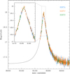 |
Fig. 1 Lensing light curve of KMT-2018-BLG-1976. The inset shows the zoomed-in view of the peak region. |
Lensing parameters of KMT-2018-BLG-1976.
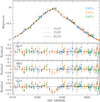 |
Fig. 2 Enlarged view in the peak region of the KMT-2018-BLG-1976 light curve. The three lower panels show the residuals from the three tested models under 1L1S, 1L2S, and 2L1S interpretations. The 2L1S model is based on the wide binary-lens interpretation. The curve drawn in the 1L1S residual panel is the difference between the 2L1S and 1L1S models. |
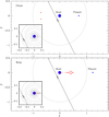 |
Fig. 3 Lens system configuration of KMT-2018-BLG-1976. The line with an arrow indicates the source trajectory,the two blue dots marked by “host” and “planet” are lens positions, and red figures represent caustics. The dotted circle around the host represents the Einstein ring. The inset shows the zoomed-in view of the central magnification region, in which the gray curves around the position of the host represent equi-magnification contours The upper and lower panels are for the “inner” (close; s < 1.0) and “outer” (wide; s > 1.0) solutions, respectively. |
3.2 KMT-2018-BLG-1996
The lensing light curve of KMT-2018-BLG-1996 is shown in Fig. 4, in which the enlarged view around the peak region is shown in the inset. The event shares a common characteristic with KMT-2018-BLG-1976 in the sense that the light curve appears to be approximated by a 1L1S curve, and a short-lasting smooth anomaly appears around the peak. The estimated lensing parameters from 1L1S modeling are (u0, tE) ~ (0.019, 45.7 days), and thus the source flux was magnified by Apeak ~ 53 at the peak. The full 1L1S lensing parameters are listed in Table 3. The data near the peak exhibit deviations, which lastedfor about 4 days, from the 1L1S model. We present the enlarged view of the peak region and the residuals from the 1L1S model in Fig. 5. The residuals of the 1L1S model exhibit a pattern similar to that of the event KMT-2018-BLG-1976: a central dip with negative deviations and bumps with positive deviations before and after the central dip.
In order to find the origin of the anomaly, we tested both the 1L2S and 2L1S models. The lensing parameters of the solutions from these modelings are listed in Table 3 along with the χ2 values of the model fits. As in the case of KMT-2018-BLG-1976, the 2L1S modeling yields two solutions, and the degeneracy between the two solutions is very severe, with Δχ2 = 0.08. The 2L1S solutions provide better fits than the 1L1S and 1L2S models, with Δχ2 = 203.8 and 54.6, respectively. The estimated binary lens parameters are (s, q) ~ (0.67, 1.69 × 10⁻³) for the close solution and ~(1.46, 1.51 × 10⁻³) for the widesolution, and thus the companion to the lens is a planetary mass object regardless of the solution. In Fig. 5, we present the model curves and residuals from the 1L2S and 2L1S (wide) models.
In the upper and lower panels of Fig. 6, we present the lens system configurations of the close and wide 2L1S solutions, respectively. From the comparison of the configurations with those of KMT-2018-BLG-1976 presented in Fig. 3, it is found that the origin of the anomaly is very similar to that of KMT-2018-BLG-1976 in the sense that it arises from the source crossing the magnification trough that extends out from the host in the direction opposite to the planet. The configuration of KMT-2018-BLG-1996 shows two important differences from that of KMT-2018-BLG-1976. First, the lens-source impact parameter, u0 ~ 0.018, is substantially smaller than that of KMT-2018-BLG-1976, with u0 ~ 0.14. Thus, in contrast to OGLE-2018-BLG-1976, the anomaly is restricted to the immediate vicinity of the central caustic, where we expect the tight mathematical correspondence between the tidal expansion (of the wide solution) and the quadrupole expansion (of the close solution) to hold (Dominik 1999; An 2005). Indeed, in contrast to OGLE-2018-BLG-1976, the central caustics are nearly identical for the two solutions, and sw × sc = 0.98 (i.e., close to unity). Second, the source passes the binary axis with a steeper source trajectory angle, α ~82°, and this results in well-developed positive deviations at both sides of the negative-deviation region, while only a single bump is seen in the anomaly of KMT-2018-BLG-1976, for which α ~61°.
In light of the relatively long timescale of the event, tE ~ 47 days, and the relatively good photometry of the observed light curve, we checked the possibility of measuring πE by conducting an additional modeling that considered the microlens-parallax effect. In the modeling, we also took into account the lens-orbital effect that may correlate with the microlens-parallax effect (Batista et al. 2011; Skowron et al. 2011). From this modeling, we find that it is difficult to constrain πE for two reasons. First, the fit improvement with the consideration of the higher-order effects, Δχ2 < 1.0, is negligible. Second, the uncertainty of the measured πE is too big to constrain the physical lens parameters. This is shown in Fig. 7, in which we present the scatter plot of points in the MCMC chain on the πE,E–πE,N parameter plane. Here, πE,E and πE,N denote the eastern and northern components of the microlens-parallax vector, πE. In the plot, the red, yellow, green, cyan, and blue colors are used to denote points with ≤ 1σ, ≤ 2σ, ≤ 3σ, ≤ 4σ, and ≤ 5σ, respectively.The scatter plot shows that the model with higher-order effects is consistent with a static model and that the uncertainty of the πE measurement, especially the northern component of the parallax vector, is too big for any meaningful constraint of the physical lens parameters.
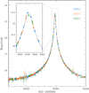 |
Fig. 4 Light curve of KMT-2018-BLG-1996. The zoomed-in view of the peak region is shown in the inset. |
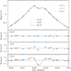 |
Fig. 5 Zoomed-in view in the peak region of the KMT-2018-BLG-1996 light curve. Notations are the same as those in Fig. 2. The 2L1S model is for the wide solution with s > 1.0. |
Lensing parameters of KMT-2018-BLG-1996.
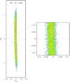 |
Fig. 7 Scatter plot of points in the MCMC chain on the πN,E–πN,N parameter plane obtained from the 2L1S modeling of the KMT-2018-BLG-1996 light curve considering higher-order effects. Red, yellow, green, cyan, and blue are used to denote points with ≤ 1σ, ≤ 2σ, ≤ 3σ, ≤ 4σ, and ≤ 5σ, respectively. |
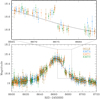 |
Fig. 8 Light curve of OGLE-2019-BLG-0954. The inset shows the enlargement of the anomaly region. |
3.3 OGLE-2019-BLG-0954
Figure 8 shows the lensing light curve of the event OGLE-2019-BLG-0954. We note that the photometric quality of the data is low due to the faintness of the source, and thus we binned the data with a 12 h interval to better show the anomalous nature of the light curve. The upper panel shows the zoomed-in view of the region around the anomaly centered at the bump at HJD′~ 8675. The anomaly exhibits ~0.3 mag deviation from the 1L1S model, which is marked by a solid curve drawn over the data points. The anomaly lasted for about 7 days, and it displays both positive (before the bump) and negative (after the bump) deviations. The light curve is similar to those of the previous two events in the sense that the anomaly does not exhibit a prominent caustic-crossing feature. The major difference is that the anomaly does not appear around the peak region but rather on the falling side of the light curve about ~ 13 days after the peak at t0 ~ 8662. The magnification of the event is low, with A ~ 2.4, and the apparent source brightness at the peak is about 0.5 mag brighter than the baseline, with Ibase ~ 19.01. The impact parameter of the source trajectory estimated from the 1L1S modeling is u0 ~ 0.4. In Table 4, we list the 1L1S lensing parameters.
In order to explain the anomaly, we tested both the 1L2S and 2L1S models. We note that the modeling was done with all data, not using the binned data, although the light curve in Fig. 8 is shown with binned data. The full lensing parameters of these solutions are listed in Table 4, and the model curves and residuals around the anomaly region are shown in Fig. 9. Similar to the previous two events, it is found that the 2L1S model with a planetary-mass companion provides a better fit than the 1L1S and 1L2S models, with Δχ2 = 423.9 and 985.0, respectively. The estimated planet/primary mass ratio between the lens components is q ~ 0.017, indicating that the mass of the lens companion is in the planetary regime. The event is different from the two previous events in two respects. First, the anomaly was produced by the caustic crossing of a source, although the caustic-crossing feature was not covered by the data. Second, the solution is uniquely determined without any degeneracy. As we mention below, the anomaly was produced by the source star crossing over the planetary caustic induced by a planet with s < 1.0. In this case, there is, in general, no degeneracy between the solutions with s < 1.0 and s > 1.0 because the planetary caustics induced by a close and a wide planet are different from each other, both in number and shape (Han 2006).
Figure 10 shows the configuration of the lens system. It shows that the planetary signal was produced by the source crossing over one of the two sets of the tiny planetary caustics produced by the planet with a normalized separation of s ~ 0.74. The duration of the caustic crossings, as measured by the time gap between the caustic entrance and exit, is ~ 7.7 h on the day of HJD′ = 8675 according tothe model. This time corresponded to night in Australia, at which point the sky was clouded out and thus no observation was conducted. Although not resolved, the caustic crossings of the source are supported by the positive deviation, which lasted for about 4.5 days during 8670.0 ≲HJD′≲ 8674.5, before the caustic crossings, and the negative deviation, which lasted for ~ 2.5 days during 8675.5 ≲HJD′≲ 8678.0, after the caustic crossings. (See the curve of the difference between the 2L1S and 1L1S models presented in the bottom panel of Fig. 9, which shows the rapid rise and fall of the 1L1S residual around the times of the caustic crossings.)
Another important difference between OGLE-2019-BLG-0954 and the other events is that it is possible to place an upper limit on the normalized source radius despite the fact that the detailed caustic-crossing feature was not resolved by the data. This can be seen in Fig. 11, where we present the scatter plot of MCMC points on the u0 –ρ plane. It shows that the upper limit of the normalized source radius is ρmax ~ 1.3 × 10⁻³ as measured at 3σ. As we show in Sect. 5, the upper limit of ρ provides an important constraint on the location of the lens.
In Fig. 12, we present the cumulative distributions of Δχ2 with respect to the 1L1S models for the individual lensing events. The light curves in the upper panels are inserted to show the region of the fit improvement. For each event, we present two cumulative distributions, where the solid and dotted curves represent 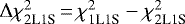 and
and 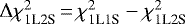 , respectively. Although the strength of the planetary signal, 40 ≲ Δχ2 ≲ 985, varies depending on the events, the distributions show that the improvement of the fit occurs at the time of the anomaly, indicating that the anomaly is a short-term perturbation, which can be explained by either a 2L1S or a 1L2S model. The fact that the 2L1S solutions provide better fits than the 1L2S solutions clearly indicates that the anomalies are of planetary origin.
Lensing parameters of OGLE-2019-BLG-0954.
 |
Fig. 9 Model curves and residuals of the 1L1S, 1L2S, and 2L1S solutions in the region around the anomaly of OGLE-2019-BLG-0954. Notations are the same as those in Fig. 2, except that the range of the residuals, −0.15–0.29 in magnitudes, is asymmetric to better show the residual from the 1L1S model. |
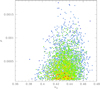 |
Fig. 11 Scatter plot of points in the MCMC chain on the u0–ρ parameter plane obtained from the 2L1S modeling of the OGLE-2019-BLG-0954 lensing light curve. The colors of the points are defined in the same way as in Fig. 7. |
4 Source stars
In this section, we specify the source stars of the events. In general, the main purpose of the source characterization is to estimate the angular Einstein radius, which helps to better constrain the physical lens parameters. For the measurement of θE, it is required to measure the normalized source radius, ρ, from which the angular Einstein radius is measured by θE = θ*∕ρ, with the angular source radius estimated from the source color and brightness. Then, the prerequisite for the θE estimation is to measure ρ. For KMT-2018-BLG-1976 and KMT-2018-BLG-1996, the ρ parameters cannot be determined because the lensing light curves do not exhibit finite-source deformations due to the absence of caustic-crossing features. For OGLE-2019-BLG-0954, however, it is possible to place a lower limit on θE because the upper limit of ρ is constrained, that is, θE,min = θ*∕ρmax. Although θE values cannot be constrained for the events KMT-2018-BLG-1976 and KMT-2018-BLG-1996, we specify their source stars for the sake of completeness.
Figure 13 shows the locations of the source stars (blue empty circles with error bars) of the individual events in the instrumental color-magnitude diagrams (CMDs) of neighboring stars around the source stars constructed using the pyDIA photometry (Albrow 2017) of the KMTC data sets. Also marked are the centroids of the red giant clump (RGC; red filled dots). The instrumental source color, V − I, and brightness, I, are measured from the regression of V - and I-band data with the variation of the lensing magnification. For KMT-2018-BLG-1996 and OGLE-2019-BLG-0954, the quality of the V -band data is not good enough to reliably determine the source colors, although the I-band brightness issecurely determined. In order to estimate the source colors for these events, we applied the method from Bennett et al. (2008) using the Hubble Space Telescope (HST) CMD. In this method, the two sets of CMDs constructed from the ground-based and HST observations (Holtzman et al. 1998) are aligned using the RGC centroid, and then the source color is estimated as that of a star on either the main-sequence or the giant branch of the HST CMD, considering the I-band brightness difference between the source and the RGC centroid. With the measured instrumental source color and brightness, the reddening and extinction corrected values,  , are estimated from the offsets in color and brightness between the source and the RGC centroid, Δ(V − I, I), using the RGC centroid as a reference (Yoo et al. 2004) via
 (1)
(1)
where  denotes the de-reddened color and brightness of the RGC centroid, which are known from Bensby et al. (2013) and Nataf et al. (2013), respectively. In Table 5 we list the estimated the values (V − I, I),
  , and
, and  for the individual events. For OGLE-2019-BLG-0954, we additionally present the lower limits of the angular Einstein radius and the relative lens-source proper motion, μ. The value of μ is estimated from the combination of θE and tE via μ = θE∕tE.
Source properties of the three events.
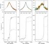 |
Fig. 12 Cumulative distributions of Δχ2 with respect to the 1L1S models for the individual lensing events. The solid and dotted distributions are
|


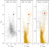 |
Fig. 13 Source positions (empty blue dots) in the instrumental CMDs. The red filled dots indicate the centroid of the red giant clump. For KMT-2018-BLG-1996 and OGLE-2019-BLG-0954, CMDs from the HST observations (brown dots) are also presented. |
5 Physical lens parameters
Although the microlens parallax is not measurable for any of the analyzed events, it is still possible to constrain the physical parameters of the lens mass and distance based on the event timescale because it is related to the physical lens parameters via
 (2)
(2)
Here, κ = 4G∕(c2AU), Mtot = M1 + M2, and DL and DS denote the distances to the lens and source, respectively. For OGLE-2019-BLG-0954, the measured lower limit of θE can place an additional constraint on the lens parameters.
We estimated the physical lens parameters by conducting a Bayesian analysis using the available constraints for the individual events. In the Bayesian analyses, we produced a large number (2 × 10⁷) of lensing events by conducting a Monte Carlo simulation using a prior Galactic model. The Galactic model is defined by the mass function and physical and dynamical distributions of Galactic objects. For the mass function of lens objects, we adopted the model defined in Jung et al. (2018). For the physical distribution, we adopted the Robin et al. (2003) model for disk objects and the Han & Gould (2003) model for bulge objects. For the dynamical distribution, we adopted the Jung et al. (2021) model, which is constructed based on the Gaia catalog (Gaia Collaboration 2016, 2018), for bulge objects, and the modified Han & Gould (1995) model for disk objects. Further details regarding the Galactic model are available in Jung et al. (2021).
Figure 14 shows the posterior distributions for the mass of the primary lens, M1, and the distance to the lens obtained from the Bayesian analysis. In each panel, the contributions from the disk and bulge lens populations are marked by blue and red curves, respectively, and the black curve is the combined contribution from the two lens populations. We mark the median value and 1σ range of the distribution by a vertical solid and two dotted lines, respectively. The uncertainty range of each parameter is estimated as the 16% and 84% of the distribution.
In Table 6, we list the estimated masses of the host and planet, the distance, and the projected planet-host separation (a⊥ = sDLθE) for the individual lenses. For KMT-2018-BLG-1976L and KMT-2018-BLG-1996L, we present paired sets of the parameters that correspond to the close and wide solutions. The estimated host and planet masses are (M1, M2) ~ (0.65 M⊙, 2 MJ) for KMT-2018-BLG-1976L, ~ (0.69 M⊙, 1 MJ) for KMT-2018-BLG-1996L, and ~(0.80 M⊙, 14 MJ) for OGLE-2019-BLG-0954L. The estimated mass of OGLE-2019-BLG-0954L is in a good agreement with the θE –M relation presented in Fig. 7 of Kim et al. (2021). According to the estimated masses, the hosts of planets are commonly K-type main-sequence stars. The fact that the lenses of all three events have similar masses can be understood by the similarity of the event timescales, ranging from tE ~ 25–29 days, which are major constraints on the determined physical parameters. We note that the mass distribution of detected lenses is different from the mass function of stars in the solar neighborhood, in which M dwarfs are about seven to eight times more common than K dwarfs; this is because the lensing probability is proportional to the size of θE, which is proportionalto M1∕2, and thus the lensing chance is higher for a lens with a higher mass. The planets KMT-2018-BLG-1976Lb and KMT-2018-BLG-1996Lb are giant planets with masses similar to and about twice the mass of Jupiter, respectively. On the other hand, the mass of OGLE-2019-BLG-0954Lb is at the planet–brown dwarf boundary2. For all lenses, the planets are located beyond the snow lines of the hosts, regardless of the type of solution (close or wide).
We note that OGLE-2019-BLG-0954L is very likely to be in the disk, while the chances for the lens to be in thedisk and bulge are roughly alike for the other two events. The constraint on the location of OGLE-2019-BLG-0954L is mostly given by the relatively large angular Einstein radius, which is ≳ 0.8 mas, combined with the high relative lens-source proper motion, which is ≳ 10.2 mas yr−1. Considering the close distance to OGLE-2019-BLG-0954L, DL ~ 3.6 kpc, we checked the possibility that a significant fraction of the blended flux comes from the lens. The expected brightness of the lens estimated from its mass, ~0.8 M⊙, and distance, DL ~ 3.6 kpc, is I ~ 19.4, assuming that the extinction to the lens is about half of the extinction toward the source star of AI ~ 2.6. This matches the estimated brightness of the blend of Ib ~ 19.5 well. Therefore, it is plausible that the lens comprises most of the blended flux. Considering that the relative lens-source proper motion is very high, this can be confirmed if follow-up observations using high-resolution instruments are conducted in the near future. Assuming that the separation for the lens-source resolution is ~ 50 mas, as demonstrated in the case of OGLE-2005-BLG-169 from the Keck adaptive optics (AO) observations conducted by Batista et al. (2015), the lens could be resolved from the source in 2024.
Physical lens parameters of the three events.
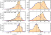 |
Fig. 14 Bayesian posteriors of the planet host mass (left panels) and distance (right panels) for the three events: KMT-2018-BLG-1976L, KMT-2018-BLG-1996L, and OGLE-2019-BLG-0954L. In each panel, the blue and red curves represent the contributions from the disk and bulge lens populations, respectively, and the black curve is the sum of the individual lens populations. The vertical solid line indicates the median of the distribution, and the two dotted lines represent the 1σ range of the distribution. |
6 Discussion
Among the three planets, one was detected via passage over a minor-image (triangular) planetary caustic (OGLE-2019-BLG-0954), one via passage near a central caustic (KMT-2018-BLG-1996), and one via passage relatively far from a resonant or near-resonant caustic (KMT-2018-BLG-1976). For random source trajectories going through the Einstein ring, the cross sections of the first two types are small because central caustics and minor-image planetary caustics are small. Indeed, it was the small size of the planetary caustic in OGLE-2019-BLG-0954 that led to it entering our sample: Small gaps in relatively dense and continuous coverage meant that there was no coverage over the short cusp crossing. However, as Yee et al. (2021) have pointed out, resonant and near-resonant caustics (defined as having “magnification-deviation ridges” of at least 10% extending from the central to the planetary caustic) have much larger cross sections, and they account for a large fraction of all planetary detections. (See their Fig. 11, which shows that roughly half of resonant or near-resonant planets are from near-resonant caustic structures.) However, for these near-resonant caustics, a substantial fraction (on the order of half) of their cross section is composed of the “10% ridge” rather than the caustics themselves. The light curves without caustic features that result from these trajectories are more likely to be missed.
Finally, we note that the comparison of the caustic diagrams of KMT-2018-BLG-1976 and KMT-2018-BLG-1996 lends credence to the conjecture of Yee et al. (2021) that the inner–outer degeneracy of planetary caustics (Gaudi & Gould 1997) and the close–wide degeneracy of central caustics (Griest & Safizadeh 1998; Dominik 1999) are limiting cases of a single continuum of degeneracies. In both cases, the light curve is characterized by a post-peak dip due to its passage over the magnification trough along the planet-host axis on the opposite side from the planet. Yet the degeneracy takes very different forms. For KMT-2018-BLG-1976 (for which the source passes much farther from the central-or-resonant caustic), the product sw × sc = 0.87 is far from unity. This is more characteristic of the inner–outer degeneracy of planetary caustics, for which one expects  , where
  is the predicted value of s based on the time of the anomaly, tanom:
 ![Mathematical equation: $u_{\textrm{anom}}^2\,{=}\,u_0^2 + [(t_0-t_{\textrm{anom}})/t_{\textrm{E}}]^2$](/articles/aa/full_html/2021/06/aa40758-21/aa40758-21-eq13.png) . For KMT-2018-BLG-1976, uanom = 0.161 and thus
. For KMT-2018-BLG-1976, uanom = 0.161 and thus  , compared to the inner–outer “prediction” of 0.87. By contrast, for KMT-2018-BLG-1996,
  , very close to the prediction of unity for the close–wide regime.
7 Summary
We have reported the discoveries of three planetary microlensing events: KMT-2018-BLG-1976, KMT-2018-BLG-1996, and OGLE-2019-BLG-0954. The planets in these events were found from the systematic reinvestigation of the microlensing events found by the KMTNet survey before the 2019 season, which was conducted to search for weak planetary signals with no obvious caustic-crossing features. Among the events, the planetary signals in KMT-2018-BLG-1976 and KMT-2018-BLG-1996 had not been previously noticed; the signal in OGLE-2019-BLG-0954 was known, but no detailed analysis had been presented. We tested various interpretations to explain the observed short-term anomalies in the lensing light curves, and this confirmed that the signals were of planetary origin. From the Bayesian analyses, it was estimated that the host and planet have masses (M1, M2) ~ (0.65 M⊙, 2 MJ) for KMT-2018-BLG-1976L, ~ (0.69 M⊙, 1 MJ) for KMT-2018-BLG-1996L, and ~(0.80 M⊙, 14 MJ) for OGLE-2019-BLG-0954L. It turned out that the lens of OGLE-2019-BLG-0954 was located in the disk and that its flux accounted for most of the blended flux. We predict that OGLE-2019-BLG-0954L will be resolved from the source when high-resolution follow-up observations are conducted in and after 2024.
Acknowledgements
Work by C.H. was supported by the grants of National Research Foundation of Korea (2019R1A2C2085965 and 2020R1A4A2002885). Work by A.G. was supported by JPL grant 1500811. This research has made use of the KMTNet system operated by the Korea Astronomy and Space Science Institute (KASI) and the data were obtained at three host sites of CTIO in Chile, SAAO in South Africa, and SSO in Australia. The OGLE project has received funding from the National Science Centre, Poland, grant MAESTRO 2014/14/A/ST9/00121 to AU.
References
- Alard, C., & Lupton, R. H. 1998, ApJ, 503, 325 [NASA ADS] [CrossRef] [Google Scholar]
- Albrow, M. 2017, https://doi.org/10.5281/zenodo.268049 [Google Scholar]
- Albrow, M., Horne, K., Bramich, D. M., et al. 2009, MNRAS, 397, 2099 [NASA ADS] [CrossRef] [Google Scholar]
- An, J. H. 2005, MNRAS, 356, 1409 [NASA ADS] [CrossRef] [Google Scholar]
- Batista, V., Gould, A., Dieters, S., et al. 2011, A&A, 529, A102 [NASA ADS] [CrossRef] [EDP Sciences] [Google Scholar]
- Batista, V., Beaulieu, J.-P., Bennett, D. P., et al. 2015, ApJ, 808, 170 [NASA ADS] [CrossRef] [Google Scholar]
- Bennett, D. P., Bond, I. A., Udalski, A., et al. 2008, ApJ, 684, 663B [Google Scholar]
- Bensby, T., Yee, J. C., Feltzing, S., et al. 2013, A&A, 549, A147 [NASA ADS] [CrossRef] [EDP Sciences] [Google Scholar]
- Bond, I. A., Bennett, D. P., Sumi, T., et al. 2017, MNRAS, 469, 2434 [Google Scholar]
- Calchi Novati, S., Suzuki, D., Udalski, A., et al. 2019, AJ, 157, 121 [Google Scholar]
- Dominik, M. 1999, A&A, 349, 108 [NASA ADS] [Google Scholar]
- Gaia Collaboration (Prusti, T., et al.) 2016, A&A, 595, A1 [NASA ADS] [CrossRef] [EDP Sciences] [Google Scholar]
- Gaia Collaboration (Brown, A. G. A., et al.) 2018, A&A, 616, A1 [NASA ADS] [CrossRef] [EDP Sciences] [Google Scholar]
- Gaudi, B. S. 1998, ApJ, 506 533 [Google Scholar]
- Gaudi, B. S., & Gould, A. 1997, ApJ, 486, 85 [Google Scholar]
- Gould, A. 1992, ApJ, 392, 442 [NASA ADS] [CrossRef] [EDP Sciences] [Google Scholar]
- Gould, A., & Loeb, A. 1992, ApJ, 396, 104 [NASA ADS] [CrossRef] [Google Scholar]
- Griest, K., & Safizadeh, N. 1998, ApJ, 500, 37 [NASA ADS] [CrossRef] [Google Scholar]
- Han, C. 2006, ApJ, 638, 1080 [NASA ADS] [CrossRef] [Google Scholar]
- Han, C., & Gould, A. 1995, ApJ, 447, 53 [NASA ADS] [CrossRef] [Google Scholar]
- Han, C., & Gould, A. 2003, ApJ, 592, 172 [NASA ADS] [CrossRef] [Google Scholar]
- Han, C., Kim, D., Udalski, A., et al. 2020a, AJ, 160, 64 [Google Scholar]
- Han, C., Udalski, A., Kim, D., et al. 2020b, A&A, 642, A110 [EDP Sciences] [Google Scholar]
- Han, C., Udalski, A., Lee, C.-U., et al. 2021, A&A, 649, A90 [EDP Sciences] [Google Scholar]
- Herrera-Martín, A., Albrow, M. D., Udalski, A., et al. 2020, AJ, 159, 256 [Google Scholar]
- Holtzman, J. A., Watson, A. M., Baum, W. A., et al. 1998, AJ, 115, 1946 [NASA ADS] [CrossRef] [Google Scholar]
- Jung, Y. K., Udalski, A., Sumi, T., et al. 2015, ApJ, 798, 123 [Google Scholar]
- Jung, Y. K., Udalski, A., Gould, A., et al. 2018, AJ, 155, 219 [Google Scholar]
- Jung, Y. K., Han, C., Udalski, A., et al. 2021, AJ, submitted [Google Scholar]
- Kim, S.-L., Lee, C.-U., Park, B.-G., et al. 2016, JKAS, 49, 37 [Google Scholar]
- Kim, D.-J., Kim, H.-W., Hwang, K.-H., et al. 2018, AJ, 155, 76 [NASA ADS] [CrossRef] [Google Scholar]
- Kim, Y. H., Chung, S.-J., Yee, J. C., et al. 2021, ArXiv e-prints [arXiv:2101.12206] [Google Scholar]
- Mao, S., & Paczyński, B. 1991, ApJ, 374, L37 [Google Scholar]
- Miyazaki, S., Sumi, T., Bennett, D. P., et al. 2018, AJ, 156, 136 [Google Scholar]
- Nataf, D. M., Gould, A., Fouqué, P., et al. 2013, ApJ, 769, 88 [NASA ADS] [CrossRef] [Google Scholar]
- Robin, A. C., Reylé, C., Derriére, S., & Picaud, S. 2003, A&A, 409, 523 [NASA ADS] [CrossRef] [EDP Sciences] [Google Scholar]
- Ryu, Y.-H., Yee, J. C., Udalski, A., et al. 2018, AJ, 55, 40 [Google Scholar]
- Shvartzvald, Y., Yee, J. C., Calchi Novati, S., et al. 2017, ApJ, 840, A3 [Google Scholar]
- Skowron, J., Udalski, A., Gould, A., et al. 2011, ApJ, 738, 87 [Google Scholar]
- Street, R. A., Choi, J.-Y., Tsapras, Y., et al. 2013, ApJ, 763, 67 [Google Scholar]
- Tomaney, A. B., & Crotts, A. P. S. 1996, AJ, 112, 2872 [NASA ADS] [CrossRef] [Google Scholar]
- Udalski, A., Szymański, M. K., & Szymański, G. 2015, Acta Astron., 65, 1 [NASA ADS] [Google Scholar]
- Woźniak, P. R. 2000, Acta Astron., 50, 42 [Google Scholar]
- Yee, J. C., Shvartzvald, Y., Gal-Yam, A., et al. 2012, ApJ, 755, 102 [NASA ADS] [CrossRef] [Google Scholar]
- Yee, J. C., Zang, W., Udalski, A., et al. 2021, AAS J., submitted [arXiv:2101.04696] [Google Scholar]
- Yoo, J., DePoy, D. L., Gal-Yam, A., et al. 2004, ApJ, 603, 139 [Google Scholar]
- Zhu, W., Penny, M., Mao, S., et al. 2014, ApJ, 788, 73 [Google Scholar]
The Extrasolar Planets Encyclopaedia (http://exoplanet.eu/).
There exist six cases of binary microlenses with companion masses at around this boundary: MOA-2010-BLG-073L (Street et al. 2013), OGLE-2013-BLG-0102L (Jung et al. 2015), MOA-2015-BLG-337L (Miyazaki et al. 2018), OGLE-2016-BLG-1190L (Ryu et al. 2018), OGLE-2017-BLG-1375L (Han et al. 2020b), and KMT-2019-BLG-1339L (Han et al. 2020a).
All Tables
All Figures
|
Fig. 1 Lensing light curve of KMT-2018-BLG-1976. The inset shows the zoomed-in view of the peak region. |
| In the text | |
|
Fig. 2 Enlarged view in the peak region of the KMT-2018-BLG-1976 light curve. The three lower panels show the residuals from the three tested models under 1L1S, 1L2S, and 2L1S interpretations. The 2L1S model is based on the wide binary-lens interpretation. The curve drawn in the 1L1S residual panel is the difference between the 2L1S and 1L1S models. |
| In the text | |
|
Fig. 3 Lens system configuration of KMT-2018-BLG-1976. The line with an arrow indicates the source trajectory,the two blue dots marked by “host” and “planet” are lens positions, and red figures represent caustics. The dotted circle around the host represents the Einstein ring. The inset shows the zoomed-in view of the central magnification region, in which the gray curves around the position of the host represent equi-magnification contours The upper and lower panels are for the “inner” (close; s < 1.0) and “outer” (wide; s > 1.0) solutions, respectively. |
| In the text | |
|
Fig. 4 Light curve of KMT-2018-BLG-1996. The zoomed-in view of the peak region is shown in the inset. |
| In the text | |
|
Fig. 5 Zoomed-in view in the peak region of the KMT-2018-BLG-1996 light curve. Notations are the same as those in Fig. 2. The 2L1S model is for the wide solution with s > 1.0. |
| In the text | |
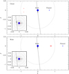 |
Fig. 6 Lens system configuration of KMT-2018-BLG-1996. Notations are the same as those in Fig. 3. |
| In the text | |
|
Fig. 7 Scatter plot of points in the MCMC chain on the πN,E–πN,N parameter plane obtained from the 2L1S modeling of the KMT-2018-BLG-1996 light curve considering higher-order effects. Red, yellow, green, cyan, and blue are used to denote points with ≤ 1σ, ≤ 2σ, ≤ 3σ, ≤ 4σ, and ≤ 5σ, respectively. |
| In the text | |
|
Fig. 8 Light curve of OGLE-2019-BLG-0954. The inset shows the enlargement of the anomaly region. |
| In the text | |
|
Fig. 9 Model curves and residuals of the 1L1S, 1L2S, and 2L1S solutions in the region around the anomaly of OGLE-2019-BLG-0954. Notations are the same as those in Fig. 2, except that the range of the residuals, −0.15–0.29 in magnitudes, is asymmetric to better show the residual from the 1L1S model. |
| In the text | |
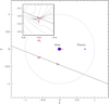 |
Fig. 10 Lenssystem configuration of OGLE-2019-BLG-0954. Notations are the same as those in Fig. 3. |
| In the text | |
|
Fig. 11 Scatter plot of points in the MCMC chain on the u0–ρ parameter plane obtained from the 2L1S modeling of the OGLE-2019-BLG-0954 lensing light curve. The colors of the points are defined in the same way as in Fig. 7. |
| In the text | |
|
Fig. 12 Cumulative distributions of Δχ2 with respect to the 1L1S models for the individual lensing events. The solid and dotted distributions are
|
| In the text | |
|
Fig. 13 Source positions (empty blue dots) in the instrumental CMDs. The red filled dots indicate the centroid of the red giant clump. For KMT-2018-BLG-1996 and OGLE-2019-BLG-0954, CMDs from the HST observations (brown dots) are also presented. |
| In the text | |
|
Fig. 14 Bayesian posteriors of the planet host mass (left panels) and distance (right panels) for the three events: KMT-2018-BLG-1976L, KMT-2018-BLG-1996L, and OGLE-2019-BLG-0954L. In each panel, the blue and red curves represent the contributions from the disk and bulge lens populations, respectively, and the black curve is the sum of the individual lens populations. The vertical solid line indicates the median of the distribution, and the two dotted lines represent the 1σ range of the distribution. |
| In the text | |
Current usage metrics show cumulative count of Article Views (full-text article views including HTML views, PDF and ePub downloads, according to the available data) and Abstracts Views on Vision4Press platform.
Data correspond to usage on the plateform after 2015. The current usage metrics is available 48-96 hours after online publication and is updated daily on week days.
Initial download of the metrics may take a while.