| Issue |
A&A
Volume 650, June 2021
|
|
|---|---|---|
| Article Number | A154 | |
| Number of page(s) | 14 | |
| Section | Extragalactic astronomy | |
| DOI | https://doi.org/10.1051/0004-6361/202140393 | |
| Published online | 24 June 2021 | |
The CaFe project: Optical Fe II and near-infrared Ca II triplet emission in active galaxies: simulated EWs and the co-dependence of cloud size and metal content
1
Center for Theoretical Physics, Polish Academy of Sciences, Al. Lotników 32/46, 02-668 Warsaw, Poland
e-mail: This email address is being protected from spambots. You need JavaScript enabled to view it.
2
Nicolaus Copernicus Astronomical Center, Polish Academy of Sciences, Bartycka 18, 00-716 Warsaw, Poland
Received:
21
January
2021
Accepted:
26
March
2021
Abstract
Aims. Modelling the low-ionisation lines (LILs) in active galactic nuclei (AGNs) still faces problems in explaining the observed equivalent widths (EWs) when realistic covering factors are used and the distance of the broad-line region (BLR) from the centre is assumed to be consistent with the reverberation mapping measurements. We re-emphasise this problem and suggest that the BLR ‘sees’ a different continuum from that seen by a distant observer. This change in the continuum reflected in the change in the net bolometric luminosity from the AGN is then able to resolve the above problem.
Methods. We carefully examine the optical Fe II and near-infrared (NIR) Ca II triplet (CaT) emission strengths with respect to Hβ emission using the photoionisation code CLOUDY and a range of physical parameters. Prominent among these parameters are (a) the ionisation parameter (U), (b) the local BLR cloud density (nH), (c) the metal content in the BLR cloud, and (d) the cloud column density. Using an incident continuum for I Zw 1 –a prototypical Type-1 narrow-line Seyfert galaxy– our basic setup is able to recover the line ratios for the optical Fe II (i.e. RFeII) and for the NIR CaT (i.e. RCaT) in agreement with the observed estimates. Nevertheless, the pairs of (U,nH) that reproduce the conforming line ratios do not relate to agreeable line EWs. We therefore propose a way to mitigate this issue. The LIL region of the BLR cloud does not see the same continuum emitted by the accretion disc as that seen by a distant observer; rather it sees a filtered version of the original continuum which brings the radial sizes into agreement with the reverberation mapped estimates for the extension of the BLR. This is achieved by scaling the radial distance of the emitting regions from the central continuum source using the photoionisation method in correspondence with the reverberation mapping estimates for I Zw 1. Taking inspiration from past studies, we suggest that this collimation of the incident continuum can be explained by the anisotropic emission from the accretion disc, which modifies the spectral energy distribution such that the BLR receives a much cooler continuum with a reduced number of line-ionising photons, allowing reconciliation in the modelling with the line EWs.
Results. (1) The assumption of the filtered continuum as the source of BLR irradiation recovers realistic EWs for the LIL species, such as the Hβ, Fe II, and CaT. However, our study finds that to account for the adequate RFeII (Fe II/Hβ flux ratio) emission, the BLR needs to be selectively overabundant in iron. On the other hand, the RCaT (CaT/Hβ flux ratio) emission spans a broader range from solar to super-solar metallicities. In all these models, the BLR cloud density is found to be consistent with our conclusions from prior studies, that is, nH ∼ 1012 cm−3 is required for the sufficient emission of Fe II and CaT. (2) We extend our modelling to test and confirm the co-dependence between metallicity and cloud column density for these two ionic species (Fe II and CaT), further allowing us to constrain the physical parameter space for the emission of these LILs. Adopting the estimates from line ratios that diagnose the metallicity in these gas-rich media –which suggest super-solar values (≳5−10 Z⊙)–, we arrive at cloud columns that are of the order of 1024 cm−2. (3) Finally, we test the effect of inclusion of a micro-turbulent velocity within the BLR cloud and find that the Fe II emission is positively affected. An interesting result obtained here is the reduction in the value of the metallicity by up to a factor of ten for the RFeII cases when the microturbulence is invoked, suggesting that microturbulence can act as an apparent metallicity controller for the Fe II. On the contrary, the RCaT cases are relatively unaffected by the inclusion of microturbulence.
Key words: accretion / accretion disks / radiative transfer / methods: data analysis / galaxies: active / quasars: emission lines / galaxies: abundances
© ESO 2021
1. Introduction
The broad-line region (BLR) of active galactic nuclei (AGNs) consists of two basic components emitting the high-ionisation lines (HILs) and low-ionisation lines (LILs), and the two regions have different physical conditions and show different dynamical motion (Collin-Souffrin et al. 1988; Marziani et al. 2019a). The LILs come from a denser region closer to the mid-plane of the black hole accretion-disc system; one that is perpendicular to the spin axis of the black hole. LILs play a very important role in two aspects, the first being in black hole mass measurements using the Hβ and Mg II lines (Czerny et al. 2019; Homayouni et al. 2020; Zajaček et al. 2020, 2021; Martínez-Aldama et al. 2020). The typical values for time-lags reported for the LILs (e.g. Hβ (IP: 13.6 eV) and Mg II (IP: 15.04 eV1)) are found to be longer than those shown for the HILs (e.g. C IV (IP: 64.49 eV) and He II (IP: 54.42 eV)) from reverberation mapping studies (Peterson & Wandel 1999; Horne et al. 2021). Secondly, LILs play an important role in defining the quasar main sequence, which additionally involves the optical Fe II emission (Boroson & Green 1992; Sulentic et al. 2000; Shen & Ho 2014; Marziani et al. 2018; Panda et al. 2018, 2019a). Here, the optical Fe II emission refers to the 4434−4684 Å blend bluewards of the Hβ emission line. This definition for the optical Fe II is employed throughout this paper.
Despite their importance and huge efforts to study them, the modelling of LILs is inherently difficult (e.g. Collin-Souffrin et al. 1986; Joly 1987; Korista et al. 1997). In the case of Fe II lines, this difficulty is connected with the large number of transitions which should be incorporated into the radiative transfer computations (e.g. in CLOUDY, Ferland et al. 2017). In spectral analyses, observational (Boroson & Green 1992; Vestergaard & Wilkes 2001) and semi-empirical (Véron-Cetty et al. 2004; Kovačević et al. 2010; Garcia-Rissmann et al. 2012) templates are frequently used. The difficulty in understanding the Fe II emission has led us in search of other reliable, simpler ionic species such as Ca II and O I (Martínez-Aldama et al. 2015b, and references therein) which would originate from the same part of the BLR and have the potential to play a similar role in quasar main sequence studies. Here, the Ca II emission refers to the Ca II triplet (CaT), that is, the infrared (IR) triplet emitting at λ8498 Å, λ8542 Å, and λ8662 Å. We refer readers to Panda et al. (2020, hereafter P20) for an overview of the issue of CaT emission in AGNs and its relevance to the Fe II emission.
In P20, we compiled an up-to-date catalogue of quasars with spectral measurements of the strengths of the optical Fe II and NIR CaT emission; for example, for the Fe II, this is the measured intensity ratio of the optical Fe II blend between 4434 and 4684 Å to Hβ, denoted RFeII. Similarly, for the CaT, this refers to the intensity ratio of the CaT emission to Hβ, denoted RCaT. Our findings in P20 reinforced the existing tight correlation (Martínez-Aldama et al. 2015b) between the strengths of the two aforementioned ionic species with a higher significance. We also performed a suite of CLOUDY2 photoionisation models to derive the RFeII − RCaT correlation from a theoretical standpoint with emphasis on the important roles played by the ionisation parameter and the local cloud density. We touched upon the effect of metallicity and cloud column density and showed their marked contribution to this correlation, albeit qualitatively.
While P20 was devoted to justifying the connection between the optical Fe II and NIR CaT, there we used only the line ratios and did not address the basic problem with the LIL-emitting region, which is the inability of our model to reproduce the observed equivalent widths (EWs) of the lines. The main goal of the present paper is to match the modelled data with the observations in terms of EWs and flux ratios of the lines of these two ions, to constrain the relative location of Fe II and CaT, and to determine the metallicity required to optimise their emission strengths. Additionally, we investigate the effect of the cloud column densities (NH) on the net emission strengths of Fe II and CaT, which, for a given local mean density of the BLR cloud, can be used to estimate the size of the BLR cloud. Treatment of the metallicity and cloud column density is done in a heuristic manner and the obtained inferences are gauged against prior observed measurements for I Zw 1.
The paper is organised as follows: in Sect. 2, we describe our photoionisation modelling setup, which is line with our approach in P20. The novelty of this part of the work lies in (i) the appropriate treatment of the issue of the EWs in terms of the covering factor for the line species; and (ii) the systematic treatment of the metallicity and cloud column density, unlike P20, where we assumed only two representative cases for each entity, namely Z = 0.2 Z⊙ and 5 Z⊙ at NH = 1024 cm−2, and NH = 1024.5 cm−2 and 1025 cm−2 at Z = Z⊙. In Sect. 3, we analyse the results from the photoionisation models and check for inconsistencies with regards to the line EWs of Hβ, optical Fe II, and CaT such as those noted in P20, and propose a way to bring the results from photoionisation modelling into agreement with the observational estimates. We discuss certain aspects of the results and their implications in Sect. 4. The key findings from this study are then summarised in Sect. 5.
2. Photoionisation simulations with CLOUDY
According to the standard photoionisation theory, the ratio of the hydrogen ionising photon density to the total hydrogen density is denoted by the dimensionless ionisation parameter U, such that:
 (1)
(1)
where QH is the number of hydrogen ionising photons emitted by the central object, r is the separation between the centre of the source of ionising radiation and the illuminated face of the line-emitting medium, nH is the total hydrogen (or mean cloud) density, and c is the speed of light. All parameters are given in cgs units. In accordance with P20, we perform a suite of CLOUDY (version 17.02, Ferland et al. 2017) models3 by varying the mean cloud density, 1010.5 ≤ nH ≤ 1013 (cm−3), the ionisation parameter, −4.25 ≤ log U ≤ −1.5, and the metallicity, 0.1 Z⊙ ≤ Z ≤ 10 Z⊙, at a base cloud column density of NH = 1024 cm−2. The cloud column density command allows the user to set the size (d) of the line-emitting medium given by the relation:  , where NH and nH have their usual meaning. Other cases of cloud column densities are explored in later sections. As in P20, we use a constant shape for the ionising continuum, one that is appropriate for the nearby NLS1, I Zw 14. The bolometric luminosity of I Zw 1 is Lbol ∼ 4.32 × 1045 erg s−1. This is obtained by applying the bolometric correction prescription from Netzer (2019):
 (2)
(2)
where, c = 40 and d = −0.2, and L5100 is measured in erg s−1. For I Zw 1, L5100 ∼ 3.48 × 1044 erg s−1 (Persson 1988). Huang et al. (2019) performed the first reverberation mapping campaign for this source and obtained a value for the L5100 = 3.19 erg s−1 which agrees well with the previous estimate from Persson (1988) within 1σ uncertainty. As we also use the RFeII and RCaT estimates from their study (Persson 1988), we incorporate their L5100 value for our study.
Compared to the range of nH and U explored in P20, both entities are extended by 1 dex to explore possible solutions in a low-density and low-ionisation regime. As opposed to P20 (where we additionally included dust in the BLR), in this paper we do not impose any limitation on the log U − log nH space. The model assumes a distribution of cloud densities at various radii from the central illuminating source to mimic the gas distribution around the close vicinity of the AGN. The range of metallicities incorporated here is inspired by the works on the quasar main sequence, where a distribution of quasars is used ranging from the low-RFeII ‘normal’ Seyfert galaxies, which can be modelled with a sub-solar assumption, to the narrow-line Seyfert galaxies (NLS1s), especially the extreme Fe II emitters, which are proposed to have super-solar metallicities (Laor et al. 1997a; Negrete et al. 2012; Marziani et al. 2019a; Śniegowska et al. 2021). Also, the range of cloud column density used is in agreement with previous works, mainly in Ferland & Persson (1989), Matsuoka et al. (2007, 2008), and Negrete et al. (2012) and further extension shown in P20. The line fluxes and RFeII and RCaT estimates are extracted from these simulations.
In the following sections, we analyse the results from the photoionisation models and check for inconsistencies with regards to the line EWs of Hβ, optical Fe II, and CaT. We then apply a simple radiation filtering to the incident continuum to mimic the incoming radiation seen by the BLR cloud which scales down the radial distance of the BLR cloud in agreement with the reverberation mapping results. This filtering also brings the EWs and their corresponding covering factors into consistency with the observed data. Next, by imposing an additional constraint on the obtained estimates for RFeII and RCaT from the photoionisation models to the observations, we are left with a small set of solutions that agree on all three counts mentioned above.
3. Results
3.1. First analysis
The results from our base setup are shown in Fig. 1. The panels in this figure show the log U − log nH parameter space colour-coded as a function of the flux ratios (RFeII or RCaT). The five panels show the setup as a function of increasing metallicity content considered in the BLR cloud model, that is, Z = 0.1 Z⊙, 0.3 Z⊙, Z⊙, 3 Z⊙, and 10 Z⊙. These figures are constructed from models that take into account a cloud column density of NH = 1024 cm−2. We illustrate the effect of other cloud column densities in Sect. 3.5. We note that U represents the ionisation parameter of the medium, and we later discuss whether or not its value should be estimated directly from the observed continuum.
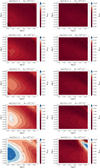 |
Fig. 1. Left: log U − log nH 2D histograms colour-weighted by RFeII with column density, NH = 1024 cm−2 shown as a function of increasing metallicity (in log-scale and in units of Z⊙). Right: physical parameters are identical to the left panels. Plots are colour-weighted by RCaT. |
In Fig. 1, for the lowest metallicity case (log Z [Z⊙] = −1, top-left panel), the maximum RFeII recovered is ∼0.575 (for log U = −1.75, log nH = 12.25). For log Z[Z⊙] = −0.5, this maximum rises to ∼0.906 (for log U = −1.75, log nH = 12). This value of maximum RFeII further increases when the metallicity is raised to solar and super-solar values. At solar metallicity, the maximum RFeII recovered is ∼1.742 (for log U = −1.75, log nH = 11.75), which is quite close to the estimate for I Zw 1 by Persson (1988) of 1.778 ± 0.050. To recover the Marinello et al. (2016)RFeII estimate, which is 2.286 ± 0.199, we assume metallicity values that are higher than solar values. For log Z [Z⊙] = 0.5 and log Z [Z⊙] = 1, we recover values for RFeII ∼ 3.296 (for log U = −1.75, log nH = 12) and ∼6.501 (for log U = −1.5, log nH = 12). Hence, from this base model analysis, we find that we can indeed recover the RFeII estimates that are consistent with the highest Fe II emitters under the assumption that the average metal content in the BLR cloud be Z⊙ ≲ Z ≲ 3 Z⊙.
Similarly, for the RCaT cases (right panels in Fig. 1), for the lowest metallicity case, log Z [Z⊙] = −1, the maximum RCaT recovered is ∼0.264 (for log U = −4.25, log nH = 12.5). This value of RCaT is obtained for the log U that is at the grid boundary. In order to assess this issue, we ran a sub-grid, going down by 1 dex until log U = −5.25. For values lower than log U = −4.25, we start to see a saturation and the recovered RCaT begins to plummet after this boundary value of −4.25. Hence, we keep this limit as it is and proceed further with our analysis. For log Z [Z⊙] = −0.5, this maximum rises to ∼0.389 (for log U = −4.25, log nH = 12.75). This value of maximum RCaT further increases when the metallicity is raised to solar and super-solar values. At solar metallicity, the maximum RCaT recovered is ∼0.557 (for log U = −4.25, log nH = 12.5), which is quite close to the estimates for I Zw 1 reported by Persson (1988) and Marinello et al. (2016) of 0.513 ± 0.130 and 0.564 ± 0.080, respectively. Requesting higher-than-solar metallicities in the case of RCaT recovers values that are yet to be confirmed observationally. Hence, from this base model analysis, we find that we can indeed recover the RCaT estimates that are consistent with the observed estimates if we take into account approximately solar metallicity values.
3.2. The problem of the EWs and covering factors in the LIL region
These results are in line with our conclusions obtained in P20, where we showed that our photoionisation models can predict RFeII and RCaT based on their flux ratios, and the modelled estimates were found to be in line with the measured values from an up-to-date observational sample of 58 sources (see Table 1 in P20), Furthermore, the measured correlation (almost one-to-one) between the two ratios was matched by both the modelled and observed data. We re-affirm this in the previous section with the agreement extended to the radial distance of the BLR in terms of the emitting regions of these two ions.
However, the proper model should reproduce not only the line ratios but also the line intensities, which are reflected in the line EWs. Therefore, we now also measure the line EWs from the grid of models. To do so, we use continua that are possibly close to the lines under consideration. For estimating the EWs for Hβ and Fe II, we use one of the CLOUDY default continuum values, at λ = 4885.36 Å. We checked for differences with the habitually considered continuum level, that is at 5100 Å, and found good agreement (they differ by ∼0.2%). On the other hand, for the CaT emission, the triplet is located in the NIR part of the spectrum, and therefore a different continuum level is required to properly estimate the EWs. This was required in previous observational works (see e.g. Martínez-Aldama et al. 2015b; Marinello et al. 2016) because of the additional contamination of the disc continuum by the reprocessed torus contribution. To mitigate this issue, we use another default CLOUDY continuum at λ = 8329.68Å, which is closer to the triplet and overlaps with the continuum windows in the NIR used in prior studies.
To estimate the covering factors for Fe II and Hβ predicted by CLOUDY, we first derive an average EW estimate from observations of a large sample of quasars that have similar physical properties to I Zw 1. We consider a subset of the DR14 Quasar Catalogue (Rakshit et al. 2020) wherein the selected subset contains quasars that have FWHM(Hβ) ≤ 4000 km s−1, which are also referred to as Population A sources. Population A sources can be understood as the class that includes local NLS1s as well as more massive high accretors which are mostly classified as radio-quiet (Marziani & Sulentic 2014) and have FWHM(Hβ) ≤ 4000 km s−1. Previous studies found that the Population A sources typically have Lorentzian-like Hβ profile shapes (Sulentic et al. 2002; Zamfir et al. 2010), in contrast to Population B sources, which have broader FWHM(Hβ) (≥4000 km s−1), are pre-dominantly ‘jetted’ sources (Padovani et al. 2017), and have been shown to have Hβ profiles that are a better fit with Gaussian (for sources with still higher full width at half maxima (FWHMs), we observe disc-like double Gaussian profiles in Balmer lines). This subset from Rakshit et al. (2020) contains 48 017 sources (about 9% of the total number of sources in the DR14 catalogue). In addition to the FWHM limit, which limits the sources within the Population A type (Marziani et al. 2018, and references therein), we employ a quality cut on the estimated EWs from the catalogues by limiting the errors associated with the EW(Hβ) measurements within 20%. This reduces the sample to 28 252 sources. The estimated mean and standard deviation values (in Å) for this subset are 48.84 and 52.42 for Fe II and 68.13 and 46.90 for Hβ, respectively. We also estimated the mean and standard deviation for the EWs for the Hα measurements in this subset which gave us 299.05 and 141.67, respectively. Going by the arguments for the typical values for the Balmer decrement in AGNs (here, Hα/Hβ) ≈ 3 (see Fig. 3 in Dong et al. 2008) we recover an average EW for Hβ of ≈100 Å given the EW(Hα). Therefore, for simplicity, we assume a generic value of 40 Å for EW(Fe II) and 100 Å for EW(Hβ) in our study. These generic values are confirmed by the sample of 58 sources in P20 containing the observations from Persson (1988), Martínez-Aldama et al. (2015a, b), and Marinello et al. (2016, 2020).
To compare the observed EWs to the model predictions we require a certain covering fraction (or factor) that scales the modelled EWs. The covering factors associated with the line species are grossly over-predicted: for Hβ, the derived EWs from the models are quite low, requiring covering factors ≳100% for 547 out of the 660 models (these 660 models include all five metallicity cases) to be comparable to the observed values. This implies that most of the model predictions of line intensities are lower by up to two orders of magnitude recovered from these models. In the following section, we propose a way to mitigate this issue and to recover EWs from the models with reasonable covering factors.
3.3. A simple proposition
We consider three cases of covering factor for the LIL region that have a typical EW(Fe II) = 40 Å recovered for Population A-type sources: at 30%, 45%, and at a more liberal 60%. These values for the covering factors of the LIL region are representative and agree with the values from the traditional single-cloud and the locally optimised cloud (LOC) models (Baldwin et al. 1995; Korista & Goad 2001). The need for high covering factors is substantiated to explain the strengths of the emission lines in the BLR and the lack of the Lyman continuum absorption suggesting a flattened distribution of the BLR and the distant observer seeing the source at relatively small viewing angles (Gaskell 2009, see also Fig. 7 in the current paper). The results of previous studies have suggested that the covering factors of the BLR and the torus are similarly based on the following reasoning: (A) If the torus had a lower covering factor than the BLR we would see the BLR in absorption against the central continuum source in some objects near the type-2 viewing position. This is never seen. (B) On the other hand, if the BLR had a lower covering factor, some regions of the dusty torus would see direct radiation from the central source. This cannot be the case for much of the torus because it would then be unable to exist as close in as is seen (Gaskell et al. 2007; Gaskell 2009, and references therein). We therefore assume here that the covering factors for the two entities (the LIL region and the torus) are similar and substantiate the assumed covering factors from prior statistical studies on large quasar samples to recover the covering factors for the torus. Previous observational studies estimated the covering factors, for example by using the ratio of IR to optical-UV luminosity (Roseboom et al. 2013) for luminous type 1 (or unobscured) quasars from large surveys in those wavebands. These latter authors estimate a mean value for the covering factor of 0.39 . On the other hand, Gupta et al. (2016) consider the ratio of the mid-IR luminosity to the bolometric luminosity to estimate the covering factors for a sample of radio-loud and radio-quiet sources. For their radio-quiet sample, these authors estimate a median covering factor of ∼0.29. In addition to these estimates, Mor et al. (2009) estimated the covering factor for I Zw 1 to be ∼63%. This was achieved by fitting the Spitzer/IRS (2−35 μm) spectrum for the source using a clumpy torus model in addition to models for dusty narrow line region clouds and dust, where the latter was modelled using a black-body distribution.
The locations of the solutions that agree with the EWs in addition to the observed flux ratios are shown in Fig. 2 using special symbols5. The underlying grid is identical to the respective panels shown already in Fig. 1. We find that the solutions for RFeII are only plausible now at higher metallicities, of the order of ∼10 Z⊙. This is in line with the observational evidence suggesting super-solar metallicities in excess of 10 Z⊙ (Hamann & Ferland 1992; Shin et al. 2013; Śniegowska et al. 2021). Models with lower metallicity values (Z ≲ 3 Z⊙) require covering factors that are above the requested limit (> 60%) and henceforth are not considered. On the other hand, for CaT emission, the flux ratios can still be produced from models that are at solar metallicities, although the covering factor required in such cases is higher (≳45%). Increasing the metallicity to higher than solar, we have more optimal solutions in terms of low covering factor (see lower panels in Fig. 2). For completeness, we also check for plausible solutions at higher than 10 Z⊙ by considering two additional cases: at 20 Z⊙ and 100 Z⊙. We notice that in 20 Z⊙ models (see Fig. 3), the solutions for RFeII are pushed to lower ionisation parameters albeit at similar densities. There are limited solutions for the RCaT case; these suggest radial sizes lower than RFeII by a factor of two, and smaller than the Hβ reverberation mapping estimate. There are no solutions that are in agreement for any of the three chosen covering factors for the 100 Z⊙ metallicity case. Hence, an increase in the metallicity up to ∼20 Z⊙ values works well for RFeII estimates in the case of I Zw 1-like sources but not for corresponding RCaT emission. For the RCaT emission, metallicity values Z ≲ 10 Z⊙ are found to be suitable to explain the EWs and the flux ratios. In summary, the solutions that reproduce agreement on both optimal EWs and the flux ratios are obtained without significant change in the density, log nH ∼ 11.75. However, the new solutions are now nearly 2 dex lower in the ionisation parameter for RFeII, that is, log U ∼ −3.5 (the maximum value for RFeII in the left panels of Fig. 1 correspond to log U ∼ 1.75).
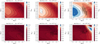 |
Fig. 2. Three cases of metallicity (Z⊙, 3 Z⊙, and 10 Z⊙) models, previously shown in Fig. 1 for RFeII (upper panels) and RCaT (lower panels), respectively. Additionally, we overlay the solutions that are in agreement with the EWs of the corresponding lines considering three representative covering factors (30% – ‘+’, 45% – ‘×’, and 60% – ‘°’). |
Next, to assess the radial size of these emitting regions, we investigate the coupled distribution between the ionisation parameter and local cloud density. As has been previously explored in Negrete et al. (2012, 2014) and Marziani et al. (2019b) and in P20, we take the product of the ionisation parameter and the local cloud density (U ⋅ nH); this entity bears resemblance to ionising flux, and for a given number of ionising photons emitted by the radiating source can be used to estimate the size of the BLR (RBLR):
![Mathematical equation: $$ \begin{aligned} R_{\rm BLR}^\mathrm{PM}\;\mathrm{[cm]} = \sqrt{\frac{Q(H)}{4\pi Un_{\rm H}c}} \equiv \sqrt{\frac{L_{\rm bol}}{4\pi h\nu \ Un_{\rm H}c}} \eqsim \frac{2.294\times 10^{22}}{\sqrt{Un_{\rm H}}}, \end{aligned} $$](/articles/aa/full_html/2021/06/aa40393-21/aa40393-21-eq6.gif) (3)
(3)
where RBLR is the distance of the emitting cloud from the ionising source which has a mean local density, nH, and receives an ionising flux that is quantified by the ionisation parameter, U. Here, Q(H) is the number of ionising photons, which can be equivalently expressed in terms of the bolometric luminosity of the source per unit energy of a single photon, that is, hν. Here, we consider the average photon energy, hν = 1 Rydberg (Wandel et al. 1999; Marziani et al. 2015). The specific value of the bolometric luminosity corresponds to 1 Zw I.
The Hβ-based RBLR for I Zw 1 was estimated to be ∼1.827 × 1017 cm (=37.2 light-days) obtained from the dedicated reverberation mapping campaign for this source (Huang et al. 2019). The authors estimate the source to be a super-Eddington accretor with a dimensionless accretion rate (
 , Wang et al. 2014) = 203.9
 . In order to validate the deviation of the source from the standard RHβ − L5100 relation (Bentz et al. 2013), they estimate the contribution of the host galaxy and subsequently recover an AGN luminosity of L5100 = 3.19
 erg s−1. This value for the AGN luminosity of the source is well within the estimate from Persson (1988) of L5100 = 3.48 × 1044 erg s−1 within 1σ uncertainty. The position of this source on the RHβ − L5100 diagram (see Fig. 4 in Huang et al. 2019) is almost at the boundary of the quoted scatter in the RHβ − L5100 relation by Bentz et al. (2013), which is at 0.19 ± 0.02 dex. This is also reflected in the conclusion of Huang et al. (2019), who state that the source follows the empirical RHβ − L5100 relation.
On the other hand, the super-Eddington accretors have been found to show shorter lags compared to their low-accreting counterparts, which brings into question the validity of the standard RHβ − L5100 relation for these sources (Du et al. 2016; Yu et al. 2020). Corrections have been proposed to the standard RHβ − L5100 relation, for example, linking to a dependence on accretion rate (Du et al. 2016; Martínez-Aldama et al. 2019) and suggestion of a ‘new’ RHβ − L5100 relation are being put forward, which uses observables such as RFeII (Du & Wang 2019) and RCaT (Martínez-Aldama et al. 2021). We test the hypothesis that this new RHβ − L5100 relation including RFeII is suitable for I Zw 1. We use the two epochs of spectral information containing the RFeII estimate from Persson (1988) and Marinello et al. (2016), i.e. 1.778 ± 0.050 and 2.286 ± 0.199, respectively. For the earlier epoch, we set the L5100 luminosity to 3.48 × 1044 erg s−1 and recover the Hβ-based RBLR ≈ 18.68 light-days for RFeII ≈ 1.778. Next, for the more recent epoch, we set the L5100 luminosity to 3.19 × 1044 erg s−1 as per Huang et al. (2019) and get the RBLR ≈ 11.93 light-days for the RFeII ≈ 2.286. Both these RBLR estimates indicate that the lags thus obtained from this new RHβ − L5100 relation are shorter by up to a factor of three than the lag value reported for I Zw 1 by Huang et al. (2019). With this in mind, we consider that the standard RHβ − L5100 applies for this source and proceed accordingly.
The similarity in the location of the emitting region for Fe II and Hβ has been studied previously. The proximity of the ionisation potential for the two ions suggests that they are produced in relatively close-by regions under similar physical conditions (Panda et al. 2018, and references therein). Hu et al. (2015) found that the time delays of Hβ and optical Fe II are mostly similar, although there is scatter in their FWHM correlation, which may suggest that Fe II is emitted from a larger region relative to Hβ. Next, we therefore consider the emitting region for Fe II and Hβ to have significant overlap and for simplicity use the Hβ radius obtained from Huang et al. (2019) as a proxy for the Fe II.
Now, with the agreement on the flux ratios for Fe II and CaT, and their EWs in harmony with the observational evidence, we are left with the problem of matching the radial distances from the continuum source. We have a discrepancy between the radius of the emitting region suggested by the reverberation mapping and the one obtained using the photoionisation method. In our case, the value of the radial distance obtained using Eq. (3) for the physical parameters log U = −3.5 and log nH = 11.75 is 1.720 × 1018 cm. We call this radius  . This value reproduces the EWs for the LILs and flux ratios of the lines in agreement with the observed values. On the other hand, from the Hβ reverberation mapping of I Zw 1, we have the radial distance at 1.827 × 1017 cm. We call this radius
  . To match these radii and recover the expected ionisation parameter, the luminosity incident on the BLR cloud responsible for the line reverberation needs to be scaled. We perform this scaling by employing the scaling relation between the radius–luminosity that agrees with the low-ionisation emitting region, i.e. RBLR ∝ L0.5. Hence, we have the following relation:
 (4)
(4)
where, L and L′ are the monochromatic luminosities for the photoionisation and the reverberation method, respectively. Thus, in our case, this scaling value is ∼0.011 (i.e. only about 1% of the original AGN continuum irradiating the BLR). This simply translates back to the lowering of the ionisation parameter by nearly 2 dex in our photoionisation modelling that reproduces the flux ratios, the EWs within reasonable covering factors, and scales down the Fe II radial distance from the central source in agreement with the reverberation measurements. The implications of this filtering are discussed in Sect. 4.1.
3.4. Salient features of the Fe II and CaT emission from photoionisation
As a result of the consideration of the proper values of the line, the EW has led us to an entirely different parameter space in the ionisation parameters than in P20 and in Sect. 3.1. We now change our approach to search for the proper parameter space. We perform a three-step refinement to extract the final solutions for the log U − log nH pertaining to the two parameters RFeII and RCaT. Step 1 is matching the EWs for the Hβ, Fe II, and CaT simultaneously within the requested covering factors (30%, 45%, and 60%). Then, the selected solutions are gauged against the radial distance that is within 20%6 of the value obtained from the RHβ − L5100 for the luminosity of I Zw 1 (∼3.48 × 1044 erg s−1, Persson 1988). The last step in the refinement is matching the modelled estimates with the observed line flux ratios for both the ions RFeII and RCaT. This is what gives us the solution marked at the top of the simulation grid in Figs. 2 and 3.
The solutions that fully satisfy the observational constraints are a small subsection of the original grid, as illustrated in Figs. 2 and 3. To better demonstrate why P20 solutions with much higher ionisation parameters are favoured, we replot all solutions in Fig. 4. The grid points from three panels for metallicity at Z⊙, ∼3 Z⊙, and 10 Z⊙ for both RFeII and RCaT are extracted from the log U − log nH space and reported here in terms of the radial distance (as referred to in previous sections, the product of U and nH for a fixed ionising continuum gives the size of the line emitting region) versus the two flux ratios. The grid points are colour-coded with the corresponding ionisation parameters. First considering the RFeII cases (left panels in Fig. 4), we can see that the maximum emission in RFeII is nearly 2 dex larger, suggesting that the radial distance here is approximately ten times greater, which is explored in the previous sections. The vertical and horizontal patches in the plots indicate the RFeII estimates within 2σ of the observed estimates and the radial sizes converted into UnH scales. Here, σ is taken as the maximum value of the error quoted from the two reported estimates from Persson (1988) and Marinello et al. (2016). Such a liberal range is considered whilst keeping in mind that the observed and modelled estimates show subtle differences; for example, in the photoionisation modelling with CLOUDY, the code considers 371 levels accounting for ∼68 635 transitions for the Fe II atom, which are evaluated only up to ∼11.6 eV (Verner et al. 1999). In the analysis of the optical spectrum for I Zw 1, there is a need to supplement the fitting procedure with broad Gaussians in addition to the Fe II pseudo-continuum generated from CLOUDY to minimise the residuals (Negrete et al. 2012, Panda & Martínez-Aldama, in prep.). This difference is highlighted by the subtle discrepancies in certain Fe II line transitions belonging to the 4F group (mostly the 37 and 38 multiplets in the 4550 Å and 4580 Å wavebands). Kovačević et al. (2010) mitigate this problem by supplying line intensities found in the observational spectrum of I Zw 1 in addition to the Fe II line transitions expected from standard photoionisation involving line recombination and collisional excitation processes. We apply the same approach (values with 2σ uncertainties) while evaluating the RCaT panels. The overlapping region between the vertical and horizontal patches marks the acceptable region for the solutions to the RFeII. As can be seen from the three left panels, the solutions are in best agreement when the BLR cloud has metallicity Z = 10 Z⊙. The gradual increase in overall modelled distribution with an increase in metallicity suggests that the BLR clouds indeed require an overabundance of iron. On the other hand, for the RCaT case, solutions with relatively low ionisation parameters can successfully achieve the required RCaT estimates. Unlike the RFeII cases, here RCaT can be modelled with a wider range of metallicities, Z⊙ ≲ Z ≲ 10 Z⊙. Although in the higher-than-solar metallicity cases, the solutions that belong to the inter-junction of the appropriate radial distances and observed RCaT values in the plots show an increasing number of solutions that prefer higher ionisation parameters (log U ≳ −4.0). These trends reveal that the emitting regions of the two species (Fe II and CaT) show significant overlap, although the results from this analysis suggest that the BLR cloud needs to be selectively overabundant in iron in order to optimize the Fe II emission. In contrast, sufficient CaT emission can be produced in a wider range of abundances ranging from solar to super-solar values. This points toward different formation channels for the two species, because iron is predominantly formed out of Type Ia supernovae (SNe) with CO-rich white dwarf progenitors, while calcium which is an α-element, is mostly produced by Type II SNe after the explosion of massive stars (7 M⊙ ≲ M* ≲ 100 M⊙, Hamann & Ferland 1993). This aspect of the study is explored in detail in a separate work (Martínez-Aldama et al. 2021) using the observational sample compiled in P20.
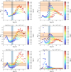 |
Fig. 4. Non-monotonic behaviour of RFeII versus log UnH colour-coded with respect to log U (left panels). Corresponding cases for RCaT are shown in the right panels. The panels represent the three sets of high-metallicity cases: log Z[Z⊙]: 0 (top), 0.5 (middle), and 1 (bottom). The pale-blue vertical strip identifies the UnH product yielding the reverberation-based RBLR (black dashed line) within the uncertainties. The pale-orange horizontal strip identifies the observed RFeII and RCaT values (black dashed lines) from Persson (1988) and Marinello et al. (2016) within uncertainties. A column density of NH = 1024 cm−2 is assumed. |
3.5. Co-dependence of metallicity and cloud column density
In P20, we explored, in a rather limited manner, the increasing trend of RFeII and RCaT estimates as a function of increasing column density. We considered two additional cases in terms of column density apart from the base value of NH = 1024 cm−2, namely 1024.5 and 1025 cm−2, limiting our models within the realms of the optically thin regime, that is, the optical depth (τ = σT ⋅ NH), τ ∼ 1−2 for optically thin medium, which implies NH ∼ 1024 − 1024.5 cm−2. Here, σT is the Thompson’s scattering cross-section and NH is the cloud column density. There is a clear hint that the real scenario perhaps points towards a collective increase in both metallicity and cloud column density. This supports the arguments in favour of using very high metallicities (Z ≳ 5 Z⊙) to recover the RFeII estimates for the strong Fe II emitters (Nagao et al. 2006; Negrete et al. 2012; Śniegowska et al. 2021) which has strong implications for the BLR cloud properties, especially their density and radial distributions. In this section, we test this connection between the two aforementioned parameters in terms of the RFeII and RCaT estimates they recover.
From the analyses in the previous sections, the parameter values for ionisation and local cloud density, that is, log UnH, that best reproduce the RFeII and RCaT in agreement with the observed flux ratios, and keeping the BLR cloud within the limits of the RBLR as estimated from the reverberation mapping and constrained for the EWs (even at covering factor ∼10%), are ∼ − 3.5 and ∼11.75 (cm−3), respectively. We therefore fix these two values in the subsequent modelling and study the effect of the metallicity within Z⊙ ≤ Z ≤ 100 Z⊙ with a step size of 0.25 dex (in log-space) and the cloud column density within 1020 ≤ NH ≤ 1025 with a step size of 0.5 dex (in log-space). Here, the modelled range for metallicity is extended to higher values than are assumed above to test their relevance in the BLR LILs emission. As for the cloud column density, NH = 1023 − 1024 cm−2 is habitually used to account for the adequate emission from the LILs where the situation is relatively less dynamic compared to the low-density HILs. The HILs require a higher ionisation parameter and hence are proposed to originate from a region much closer to the black hole and bear a more direct continuum as opposed to the LILs (Leighly 2004; Negrete et al. 2012; Martínez-Aldama et al. 2015b). Also, at the expected radial extensions for the LILs, the clouds are relatively cold and can clump together. In addition, the lowering of the net radiation pressure keeps the cloud relatively extended (Marconi et al. 2008; Netzer 2009). On the other hand, having a larger cloud column allows species like Fe II to increase their ionic fraction compared to Hβ and thereby produce enough emission to account for the RFeII ≳ 1, as often seen for the high Fe II-emitters belonging to the extreme Population A (see Bruhweiler & Verner 2008; Panda et al. 2018, 2019a, and references therein).
In Fig. 5, we demonstrate the strong degeneracy between the two quantities (metallicity and cloud column density) as a function of the recovered values for RFeII and RCaT. It is clearly seen that the same value of RFeII or RCaT can be derived by widely different combinations of column density and metallicity. The main plots are in log–log space so that the large extent of the intensity ratio against the fifth-order stretch of cloud column density can be appreciated. RFeII and RCaT estimates have been reported from prior spectroscopic observations for I Zw 1: (a) RFeII and RCaT estimates from Persson (1988) are 1.778 ± 0.050 and 0.513 ± 0.130, respectively; (b) RFeII and RCaT estimates from Marinello et al. (2016) are 2.320 ± 0.110 and 0.564 ± 0.083, respectively. We use these measurements and overlay them on Fig. 5 with the quoted uncertainties in the measured values. For the RFeII case, the models that have metallicities Z ≲ 3 Z⊙ cannot account for the expected intensity ratio, not even for the lower limit from Persson (1988), even at the highest column density (1025 cm−2) considered in the analysis. We start to enter the optimal regime with Z ∼ 5 Z⊙ and higher. The inset plot zooms in on the optimal range of solutions in terms of the RFeII recovered (note the linear scale used here for the y-axis), and the column density and metallicity values needed to obtain that value. In principle, BLR cloud with the smallest size can reproduce the optimal RFeII emission, although in this case, the models require extremely high metallicity (100 Z⊙). Such an inverse behaviour between metallicity and cloud column size is no surprise because these clouds are effectively made of mostly hydrogen and helium, which exist in the front-facing part (or the fully ionised zone) of the cloud, while heavier and more metallic elements tend to occur in deeper parts of the cloud as revealed by the increase in the ionic fractions for the latter as a function of the depth within the BLR cloud (see Fig. 4 in Negrete et al. 2012). As we increase the column size, the RFeII estimate can still be obtained with lower metallicity values. For RCaT, the trend between the RCaT and cloud column density is rather monotonic in log–log space. Similar to the RFeII, smaller cloud sizes suggest higher metallicity, yet solutions with almost solar values for metallicity are sufficient to recover the required RCaT emission for cloud column sizes that are similar to the RFeII case, i.e. NH ≳ 1024 cm−2. Therefore, a degeneracy between these two quantities, that is, metallicity and cloud column density, sustains. We discuss this conundrum between the metallicity and cloud column density in the BLR clouds and highlight ways to break this degeneracy in Sect. 4.
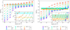 |
Fig. 5. Left: strength of the optical Fe II emission (RFeII) shown with respect to the distribution in cloud column density (NH) from CLOUDY. The model uses a log U = −3.5 and log n = 11.75. The colours represent nine different cases of metallicity (Z). The observed estimates from Persson (1988) and Marinello et al. (2016) for I Zw 1 are shown in cyan and orange bars (the errors in these estimates are depicted by the widths of the bars), respectively. The inset plot zooms in on a portion of the base plot to highlight the modelled trends that recover the RFeII within the observed values. We note that the RFeII is shown in log scale in the base plot while for the inset plot we show the ratio in linear scale. Right: corresponding RCaT distribution for the same modelled parameters as in the previous panel. |
3.6. Microturbulence: a metallicity controller?
Another important aspect to consider in the optimisation of the Fe II emission is the effect of the microturbulence, which has been noted to provide additional excitation (Baldwin et al. 2004; Bruhweiler & Verner 2008). The velocity field around a black hole might be a superposition of different kinematic components, such as Doppler motions, turbulence, shock components, in/outflow components, and rotation. Different velocity components result in different profiles, and the final profile is a convolution of different components (Kollatschny & Zetzl 2013). Furthermore, local turbulence substantially affects the Fe II spectrum in photoionisation models by facilitating continuum and line-line fluorescence. Increasing the microturbulence can increase the Fe II strength and give better agreement between the predicted shape of the Fe II blends and observation (Shields et al. 2010). The effect of microturbulence has been carefully investigated in our previous works (Panda et al. 2018, 2019b), where a systematic rise in RFeII estimates is obtained by increasing the microturbulence up to 10−20 km s−1. After this limit, the RFeII tends to drop and for 100 km s−1 reaches values similar to zero microturbulent velocity. We tested the effect of the microturbulence in the context of this study, in particular whether or not this entity works similarly for boosting the CaT. We considered a microturbulence value of 20 km s−1 and re-ran our models. The results are summarised in Fig. 6 for the two ions side by side. As expected, for the RFeII case, the microturbulence leads to comparable RFeII estimates for lower metallicity. For example, the case with no microturbulence with solar metallicity gives RFeII values similar to the microturbulence = 20 km s−1 at 0.3 Z⊙. This effect is seen in other metallicity cases as well. For the preferred solution with ∼10 Z⊙ for the case with no microturbulence, upon invoking this parameter, we achieve the solution with the ∼3 Z⊙ models. On the other hand, for the RCaT cases, the results are almost similar between the two versions, indicating that the CaT emission is probably less prone to fluorescence effects. We overlay the solutions that agree with the line EWs for the three cases of covering factors similar to Figs. 2 and 3. For a much lower covering factor (∼10%), we find that with the inclusion of microturbulence in the medium, RFeII estimates closer to those of Marinello et al. (2016) are more probable with an ionisation parameter of log U ∼ −3.5 and density of log nH ∼ 11.5, albeit at 10 Z⊙. For the same low covering factor, there is a unique solution satisfying for RCaT, i.e. for log U ∼ −3.25 and log nH ∼ 11.5 also at 10 Z⊙, which shows that the two ions can have significant overlap in their emitting regions. This is another confirmation of the nearly 1:1 correlation obtained in P20 between the RCaT and RFeII. There are solutions with higher covering factors that agree with the line EWs at metallicities Z ≲ 10 Z⊙ in the RFeII cases with ionisation parameter as high as log U ≳ −2.75, yet the cloud densities remain nearly unchanged at log nH ≳ 11.5 (cm−3). These latter solutions then require larger covering factors (> 30%) to account for the optimal emission in Fe II. The last panel of RFeII cases with microturbulence included (10 Z⊙) show significant overlap with the solutions realised from Z ≈ 20 Z⊙ models for RFeII (see Fig. 3). The effect of microturbulence is only a secondary effect seen from the spectra as this affects mostly the wings of the broad line profiles (Goad et al. 2012); the effect becomes quite difficult to estimate properly as these features become increasingly close to the noise level.
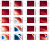 |
Fig. 6. Effect of microturbulence: The first and third columns are from the original models without any microturbulence for RFeII and RCaT, respectively. The second and fourth columns are the corresponding cases with microturbulence = 20 km s−1. Each column consists of the five cases of metallicity considered in this work. The overlaid symbols have the same meaning as shown previously in Fig. 2. |
4. Discussions
The problem in reproducing the EWs of LILs has been discussed in the literature. Several explanations are possible: additional mechanical heating is perhaps necessary (e.g. Collin-Souffrin et al. 1986; Joly 1987), or a multiple cloud approach, with part of the radiation scattered and/or re-emitted between different clouds, or the BLR does not see the same continuum as the observer (Korista et al. 1997) due to an intervening medium such as a wind component (Leighly 2004). This wind component is often seen in high-ionisation lines in the UV, such as C IV, of an AGN spectrum typically belonging to the Population A type (Marziani et al. 2018, and references therein) like I Zw 1. In our computations, we recover the proper Fe II ratio and EW for low values of the ionisation parameter which indicates that we do not need extra energy to produce stronger lines but must instead reduce the incident flux; otherwise the medium is over-ionised and line production efficiency drops. This favours the option of the intervening medium. We applied the latter hypothesis to analyse I Zw 1 and its LILs of the BLR. This scenario is also supported by the recent observational findings of Wolf et al. (2020), who found that the Fe II-emitting region is shielded from the central source for a sample of ∼2100 Type-1 AGNs (see Martínez-Aldama et al. 2015b, for a similar inference on CaT). We illustrate this scenario in Fig. 7 wherein the key assumption is that the broad-band spectral energy distribution (SED) seen by the BLR is different from the one that is perceived by a distant observer. This hypothesis can be perceived as the combined effect of (a) geometrical effects, and (b) radiation filtering due to obscuration. Nevertheless, other effects, such as lensing and limb darkening, which modify the inclination dependence, could additionally supplement in recovering this radiation filtering. The flattened disc geometry results in an inclination-dependent flux (∝ cos θ, where θ is the angle between the symmetry axis and the line-of-sight of the observer). On the other hand, the filtering, or rather the collimation of the continuum can be a result of the anisotropy in the radial structure of the disc. The anisotropy originating from the accretion disc has been suggested by previous studies (Wang et al. 2014, and references therein) pointing away from a generally assumed geometrically thin accretion disc especially in the regions at close vicinity of the black hole. Such a geometry inhibits the radiation coming from the inner, hotter region, making it possible for the BLR to receive a continuum that is a fraction of the original ionising flux. This is a valid assumption in the case where the observer is systematically at an offset in the viewing angle to the BLR cloud.
 |
Fig. 7. Schematic view of the anisotropy in the radiation between the observer and the BLR cloud. Our model considers a simple shrinking of the radial position of the BLR to match the reverberation-mapped RBLR estimate, by filtering the incoming radiation from the accretion disc. Therefore, the net SED seen by the BLR differs from the SED seen by a distant observer. This illustration applies to I Zw 1-like sources, i.e. Type-1 Narrow-line Seyfert galaxies with high Fe II emission, which are the context of this study. |
4.1. Analysing the change in the shape of the SED
A primary finding of the present study is that BLR clouds that have sizes of the order of ≈1012 cm need to see about 1% of the SED and have optimised properties in order to reproduce all the observational constraints for the LILs in extreme objects like I Zw 1. Here, we discuss the implications of these findings and their justification based on prior studies.
Wang et al. (2014) studied in detail the solutions for the structure of accretion discs from sub-Eddington accretion rates to extremely high, super-Eddington rates (where the dimensionless accretion rate,  ≫ 1). The appearance of sharper funnels in the innermost region (below 3 Rg, where Rg is the gravitational radius) as the accretion rate increases significantly modifies the thin-disc geometry that applies under the Shakura & Sunyaev (1973) regime. The authors note that the aspect ratio (h = H/r, where H is the height of the disc and r is the distance along the radial direction, both in units of Rg such that h is dimensionless) of the funnel for these slim discs is insensitive to the black hole mass and the shape of a slim disc has three notable features: (1) a funnel that develops in the innermost region [dh/dr > 0]; (2) a flattened part [dh/dr < 0 and h ∼ 1]; and (3) a geometrically thin part (h ∼ 10−2), approaching the Shakura & Sunyaev (1973) regime, in which the funnel disappears. The authors further investigate the effect of the SEDs received by the BLR (or a distant observer) with different inclinations to the disc. In the present study, the BLR clouds are considered to be relatively close to the midplane of the system (see Fig. 7) such that the inclination angles (to the symmetry axis) subtended by these clouds are relatively high, around 75−85°7. On the other hand, the face-on view of NLS1 sources such that the inclination angle subtended to the distant observer is relatively small (Wu & Han 2001; Panda et al. 2019a) is supported by the small widths of the Balmer lines due to the projection effect (Osterbrock & Pogge 1985; Bian & Zhao 2004). Recent studies by Rakshit et al. (2017) who used the SDSS DR12 data to construct an NLS1 catalogue also found that, statistically, the NLS1s have smaller viewing angles in comparison to their broad-line counterparts. In Wang et al. (2014), the authors notice the anisotropy of the radiation field clearly with their study and note that: (1) the flux received by the clouds (or the distant observer) dramatically decreases with increasing inclination by a factor of 30 (i.e. going from θ = 10° to θ = 80°), which is much steeper than what is recovered with the simple cos θ dependence; and (2) the SEDs are significantly softened by self-shadowing at higher inclinations, resulting in the lack of photoionising photons required for the emission lines. We highlight the relative change in the bolometric flux content as a function of the source’s inclination with respect to the distant observer in Fig. 8 for two sets of slim disc SEDs (at
  = 100 and 500, Jian-Min Wang, priv. comm.) at a black hole mass of 107 M⊙ similar to the estimate from Huang et al. (2019), i.e. 9.30
 M⊙. The selection of the lower value of inclination was based on the Mor et al. (2009) estimate for the viewing angle from torus fitting to Spitzer/IRS 2−35 μm spectra for I Zw 1 suggesting a value of θ ≈ 8°. We chose a SED model with θ = 10° to mimic the SED seen by a distant observer. On the other hand, for the BLR, we chose a modelled SED with a higher inclination angle (θ = 80°). We estimate the flux ratio between the two cases of inclination (θ = 10° and 80°) at 0.1 keV. The choice of the reference energy is according to Wang et al. (2014) that drives the Hβ emission. For the
  = 100 case, we obtained a flux ratio ≈96.67%. For a higher accretion rate, for example
  = 500, we obtain a value (≈99.92%) consistent with the filtering factor we obtain from the scaling of the BLR radius. These flux ratios, when estimated at 1 Rydberg give us 62.5% and 90.62% for
  = 100 and 500, respectively.
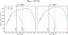 |
Fig. 8. Spectral energy distributions obtained for slim accretion discs for a representative black hole mass, MBH = 107 M⊙ for two cases of accretion rates (dimensionless): Left: |


The anisotropic emission from the accretion disc has been tested more rigorously in past studies (Runnoe et al. 2013; Xu 2015; Lasota et al. 2016, and references therein), such as in the context of estimating quasar bolometric corrections considering thin accretion discs as the source of the continuum emission including relativistic effects (Nemmen & Brotherton 2010). In such cases, the authors find a slump in the net integrated luminosity for a source over an order of magnitude when the viewing angle increases from θ = 10° to θ = 80° (see Fig. 3 in Nemmen & Brotherton 2010). The relative decrease in this luminosity as a function of the increasing viewing angle can be even higher under Newtonian approximation where the bolometric luminosity is related to the integrated luminosity assuming isotropic emission such that:
 (5)
(5)
where, ν0 and ν1 are the frequencies bounds for thin disc radiation. On the other hand, strong light-bending effects in quasar microlensing events can cause differential lensing distortion of the X-ray and the optical emission and can significantly change the X-ray-to-optical flux ratios in such sources (Chen et al. 2013).
Narrow-line Seyfert galaxies with high accretion rates are typically shown to have a soft-X-ray excess (Arnaud et al. 1985) in their broadband SED (Jin et al. 2012a,b; Marziani et al. 2018; Ferland et al. 2020). The interstellar medium blocks our view of this spectral region, thus necessitating the use of indirect methods to predict the emission from this part of the radiation field (Kubota & Done 2018, and references therein). This component helps to bridge the absorption gap between the UV downturn and the soft-X-ray upturn (Elvis et al. 1994; Laor et al. 1997b; Richards et al. 2006) and changes the far-UV and soft-X-ray part of the spectrum, affecting the Fe II line production (Panda et al. 2019b). Therefore, there is a need to expand the study to construct more realistic SEDs for I Zw 1 and similar sources which will be undertaken in subsequent work.
4.2. Degeneracies with metallicity and cloud size in the BLR
Additional constraints from high signal-to-noise-ratio rest-frame UV spectra for I Zw 1 can help narrow down the possibilities for the metallicity. There are quite a few metallicity indicators; for example, Al IIIλ1860/He IIλ1640, a fairly unbiased estimator for the metallicity (see Śniegowska et al. 2021, for an overview). Another line ratio frequently used is Si IVλ1397+O IV]λ1402/C IVλ1549 (Hamann & Ferland 1999, and references therein). The choice of diagnostic ratios used for metallicity estimates is usually a compromise between S/N, ease of deblending, and straightforwardness of physical interpretation. Laor et al. (1997a) performed a spectral decomposition of the HST-FOS spectrum of I Zw 1 and reported the various spectral parameters in their paper. The Al III/He II flux ratio from their analysis is ≈1.78 and the Si IV+O IV]/C IV gives ≈0.89, suggesting a metallicity ∼10 Z⊙ and slightly above solar, respectively. However, another ratio, N Vλ1240/He II flux ratio gives a value of ∼5.78 suggesting Z ≳ 10 Z⊙, although this ratio is quite sensitive to change in ionisation parameter (Wang et al. 2012). Other ratios, such as C IV/He II and Si IV+O IV]/He II also point towards similarly high metallicities (Z ≳ 10 Z⊙), although they are not so reliable due to issues related to blending with other species which becomes cumbersome unless better quality spectra are available. Therefore, using the Al III/He II flux ratio coupled with the photoionisation-based estimates in this work puts the column density required for RFeII at ≳1024 cm−2. More recent works suggest a slightly higher value for these line ratios; for example, Al III/He II = 5.35 ± 2.728 if the λ1900 Å blend is fitted with a combination of a blueshifted component that is characteristic of the low-density high-ionisation outflowing component, and a broad component that is typical for the high-density low-ionisation part of the BLR (Negrete et al. 2012, Paola Marziani, priv. comm.). Certainly, a higher S/N is needed to properly account for the issues mentioned above. The increased availability of optical–UV and NIR spectroscopic measurements, especially with the advent of the upcoming ground-based 10-metre-class (e.g. Maunakea Spectroscopic Explorer, Marshall et al. 2019) and 40 metre-class (e.g. The European Extremely Large Telescope, Evans et al. 2015) telescopes; and space-based missions such as the James Webb Space Telescope and the Nancy Grace Roman Space Telescope, would certainly be a welcome addition to help break this degeneracy.
On the other hand, for the cloud sizes, Ferland et al. (2009) find that the minimum column density required is ∼1023 cm−2 for gravity to overpower radiation pressure and allow infall of clouds as found by Hu et al. (2008). Using arguments based on virial determinations of the black hole mass in AGNs by Marconi et al. (2008), Netzer (2009) also concludes that the column densities must substantially exceed ∼1023 cm−2 to avoid excessive effects of radiation pressure on the orbital velocities of the BLR clouds. Thus, there may be limited freedom to vary the column density to produce the wide range of optical Fe II strength observed which then restricts the parameter space within ≲2 dex in column density without accounting for significant electron scattering effects that start to become important at higher optical depths. With such constraints on the column densities and from Fig. 5, we expect metallicities no greater than ∼30 Z⊙ but still ≳5 Z⊙ in order to efficiently produce the required RFeII values in this case. From the point of view of recent advances in observations, only very recently are we starting to resolve the inner parsec scales in nearby AGNs using interferometric techniques (GRAVITY Collaboration 2018, 2020) but mapping individual BLR clouds is something that remains elusive.
5. Conclusions
In this article, we examine the RFeII and RCaT emission in the broad-line regions of active galaxies. We probe the parameter space in terms of (a) ionisation parameter, (b) the BLR cloud density, (c) the metal content in the BLR cloud, and (d) the size of the BLR cloud in terms of the cloud column density. We incorporate the observational broad-band SED of the prototypical narrow-line Seyfert 1 galaxy, I Zw 1, which serves as the incident continuum that photoionises the BLR cloud. In our previous paper (P20) and the first attempt of this paper, we are successful in reproducing the respective flux ratios (RFeII and RCaT), although it was noticed that the pairs of log U − log nH that correspond to the best estimates for the flux ratios do not recover reasonable line EWs for these low-ionisation lines, including Hβ. We evaluate the EWs for the entire grid of models and optimise the line EWs within reasonable covering factors (between 30% and 60%) and recover the flux ratios obtained from two epochs of prior observations for this source (Persson 1988; Marinello et al. 2016). These new solutions are found to have ionisation parameters (log U ∼ −3.5) that are ∼2 dex smaller than previous results, although the local cloud density remains almost unchanged (log nH ∼ 12 cm−3). This points towards a significant reduction in the flux that is incident on the BLR cloud compared to what has been assumed before. We achieve this reduction in the flux by scaling the radial distance of this LIL-emitting region obtained from our photoionisation modelling to the radial distance obtained from the reverberation mapping estimate for I Zw 1 using the standard radius–luminosity relation (RBLR ∝ L0.5). This suggests that the broad-line region cloud does not ‘see’ the same continuum emitted from the accretion disc as that seen by a distant observer, and that rather it sees a filtered, colder continuum that implies a lowering in the number of line-ionising photons that irradiate the BLR. This in turn suggests smaller radial sizes than predicted earlier by photoionisation modelling. This screening of the accretion disc continuum can be tied to the flux as a function of the cos i, where i is the inclination angle to the symmetry axis. Additionally, there can be a lowering of the photon flux due to anisotropy in the disc structure causing self-shadowing effects as the accretion rate increases in addition to light-bending effects. Our results are applicable to Type-1 Narrow-line Seyfert galaxies with high Fe II emission, i.e. I Zw 1-like sources.
Independently from this aspect, our study still finds that the BLR needs to be selectively overabundant in iron in order to account for the adequate RFeII emission. This is suggested by the requirement of higher-than-solar metallicities (Z ≳ 10 Z⊙) to optimise the emission of optical Fe II. On the other hand, the RCaT emission spans a broader range in metallicity, from solar to super-solar metallicities. In all these models, the BLR cloud density is found to be consistent with our conclusions from prior works, i.e. nH ∼ 1012 cm−3 is required for the sufficient emission of Fe II and CaT. We further our modelling to test and confirm the co-dependence between the metallicity and the cloud column density for these two ions and constrain the effective cloud sizes using metallicity constraints from UV line ratios shown to be effective tracers of the metal content in the BLR. Finally, we test the effect of inclusion of a turbulent velocity within the BLR cloud which informs us that the RFeII emission is positively affected by the inclusion of the microturbulence parameter. An interesting result obtained here is that when the microturbulence is invoked, there is a reduction in the value of the metallicity required to obtain optimal RFeII estimates, suggesting that microturbulence can act as a metallicity controller for the Fe II. On the contrary, the RCaT cases are rather unaffected by changes in microturbulence.
The values for the ionisation potential (IP) are taken from NIST Atomic Spectra Database Ionization Energies.
N(U) × N(nH) × N(Z) = 12 × 11 × 5 = 660 models.
The I Zw 1 ionising continuum shape is obtained from NASA/IPAC Extragalactic Database.
For lower covering factors (e.g. ∼10%), we have one solution each for RFeII and RCaT, i.e. at log U = −3.5, log nH = 11.75 at log Z [Z⊙] = 1 (for RFeII), and, log U = −3.5, log nH = 11.5 at log Z [Z⊙] = 1 (for RCaT). This pair of solutions is unanimously recovered for all cases of the covering factors considered in this work.
The reported time delay for I Zw 1 in Huang et al. (2019) has an associated mean uncertainty of ∼13%.
Here the angle is estimated using the relation 90° – tan , where H′ is the peak height attained by the BLR cloud and r′ is the corresponding radial distance of the BLR cloud from the black hole. This picture of the BLR considers clouds accelerated under the combined influence of radiation pressure and gravity. We refer the readers to Naddaf et al. (2021) for more details.
Acknowledgments
I thank the anonymous referee for useful suggestions that helped to improve the paper. I would like to thank Prof. Paola Marziani for performing a re-analysis of the I Zw 1 spectrum to estimate the metallicity and Prof. Jian-Min Wang for providing his slim disc SED models for this project. I’d like to thank Prof. Bożena Czerny, Prof. Paola Marziani, Dr. Mary Loli Martínez-Aldama and Dr. Deepika Ananda Bollimpalli for fruitful discussions leading to the current state of the paper. I thank Prof. Bożena Czerny, Prof. Paola Marziani and Mr. Sushanta Kumar Panda for proof-reading the manuscript and suggesting corrections to improve the overall readability. The project was partially supported by the Polish Funding Agency National Science Centre, project 2017/26/A/ST9/00756 (MAESTRO 9) and MNiSW grant DIR/WK/2018/12. Softwares: CLOUDY v17.02 (Ferland et al. 2017); MATPLOTLIB (Hunter 2007); NUMPY (Oliphant 2015); R (R Core Team 1988).
References
- Arnaud, K. A., Branduardi-Raymont, G., Culhane, J. L., et al. 1985, MNRAS, 217, 105 [NASA ADS] [CrossRef] [Google Scholar]
- Baldwin, J., Ferland, G., Korista, K., & Verner, D. 1995, ApJ, 455, L119 [NASA ADS] [CrossRef] [Google Scholar]
- Baldwin, J. A., Ferland, G. J., Korista, K. T., Hamann, F., & LaCluyzé, A. 2004, ApJ, 615, 610 [NASA ADS] [CrossRef] [Google Scholar]
- Bentz, M. C., Denney, K. D., Grier, C. J., et al. 2013, ApJ, 767, 149 [Google Scholar]
- Bian, W., & Zhao, Y. 2004, MNRAS, 352, 823 [NASA ADS] [CrossRef] [Google Scholar]
- Boroson, T. A., & Green, R. F. 1992, ApJS, 80, 109 [Google Scholar]
- Bruhweiler, F., & Verner, E. 2008, ApJ, 675, 83 [NASA ADS] [CrossRef] [Google Scholar]
- Chen, B., Dai, X., & Baron, E. 2013, ApJ, 762, 122 [CrossRef] [Google Scholar]
- Collin-Souffrin, S., Dumnont, S., Joly, M., & Pequignot, D. 1986, A&A, 166, 27 [Google Scholar]
- Collin-Souffrin, S., Dyson, J. E., McDowell, J. C., & Perry, J. J. 1988, MNRAS, 232, 539 [NASA ADS] [CrossRef] [Google Scholar]
- Czerny, B., Olejak, A., Rałowski, M., et al. 2019, ApJ, 880, 46 [Google Scholar]
- Dong, X., Wang, T., Wang, J., et al. 2008, MNRAS, 383, 581 [NASA ADS] [Google Scholar]
- Du, P., & Wang, J.-M. 2019, ApJ, 886, 42 [NASA ADS] [CrossRef] [Google Scholar]
- Du, P., Wang, J.-M., Hu, C., et al. 2016, ApJ, 818, L14 [NASA ADS] [CrossRef] [Google Scholar]
- Elvis, M., Wilkes, B. J., McDowell, J. C., et al. 1994, ApJS, 95, 1 [Google Scholar]
- Evans, C., Puech, M., Afonso, J., et al. 2015, ArXiv e-prints [arXiv:1501.04726] [Google Scholar]
- Ferland, G. J., & Persson, S. E. 1989, ApJ, 347, 656 [NASA ADS] [CrossRef] [Google Scholar]
- Ferland, G. J., Hu, C., Wang, J.-M., et al. 2009, ApJ, 707, L82 [Google Scholar]
- Ferland, G. J., Chatzikos, M., Guzmán, F., et al. 2017, Rev. Mex. Astron. Astrofis., 53, 385 [NASA ADS] [Google Scholar]
- Ferland, G. J., Done, C., Jin, C., Landt, H., & Ward, M. J. 2020, MNRAS, 494, 5917 [Google Scholar]
- Garcia-Rissmann, A., Rodríguez-Ardila, A., Sigut, T. A. A., & Pradhan, A. K. 2012, ApJ, 751, 7 [NASA ADS] [CrossRef] [Google Scholar]
- Gaskell, C. M. 2009, New Astron. Rev., 53, 140 [NASA ADS] [CrossRef] [Google Scholar]
- Gaskell, C. M., Klimek, E. S., & Nazarova, L. S. 2007, ArXiv e-prints [arXiv:0711.1025] [Google Scholar]
- Goad, M. R., Korista, K. T., & Ruff, A. J. 2012, MNRAS, 426, 3086 [NASA ADS] [CrossRef] [Google Scholar]
- GRAVITY Collaboration (Sturm, E., et al.) 2018, Nature, 563, 657 [Google Scholar]
- GRAVITY Collaboration (Amorim, A., et al.) 2020, A&A, 643, A154 [NASA ADS] [CrossRef] [EDP Sciences] [Google Scholar]
- Gupta, M., Sikora, M., & Nalewajko, K. 2016, MNRAS, 461, 2346 [Google Scholar]
- Hamann, F., & Ferland, G. 1992, ApJ, 391, L53 [NASA ADS] [CrossRef] [Google Scholar]
- Hamann, F., & Ferland, G. 1993, ApJ, 418, 11 [NASA ADS] [CrossRef] [Google Scholar]
- Hamann, F., & Ferland, G. 1999, ARA&A, 37, 487 [NASA ADS] [CrossRef] [Google Scholar]
- Homayouni, Y., Trump, J. R., Grier, C. J., et al. 2020, ApJ, 901, 55 [Google Scholar]
- Horne, K., De Rosa, G., Peterson, B. M., et al. 2021, ApJ, 907, 76 [Google Scholar]
- Hu, C., Wang, J.-M., Ho, L. C., et al. 2008, ApJ, 687, 78 [NASA ADS] [CrossRef] [Google Scholar]
- Hu, C., Du, P., Lu, K.-X., et al. 2015, ApJ, 804, 138 [NASA ADS] [CrossRef] [Google Scholar]
- Huang, Y.-K., Hu, C., Zhao, Y.-L., et al. 2019, ApJ, 876, 102 [Google Scholar]
- Hunter, J. D. 2007, Comput. Sci. Eng., 9, 90 [NASA ADS] [CrossRef] [Google Scholar]
- Jin, C., Ward, M., & Done, C. 2012a, MNRAS, 422, 3268 [NASA ADS] [CrossRef] [Google Scholar]
- Jin, C., Ward, M., Done, C., & Gelbord, J. 2012b, MNRAS, 420, 1825 [NASA ADS] [CrossRef] [Google Scholar]
- Joly, M. 1987, A&A, 184, 33 [NASA ADS] [Google Scholar]
- Kollatschny, W., & Zetzl, M. 2013, A&A, 549, A100 [NASA ADS] [CrossRef] [EDP Sciences] [Google Scholar]
- Korista, K. T., & Goad, M. R. 2001, ApJ, 553, 695 [NASA ADS] [CrossRef] [Google Scholar]
- Korista, K., Baldwin, J., Ferland, G., & Verner, D. 1997, ApJS, 108, 401 [NASA ADS] [CrossRef] [Google Scholar]
- Kovačević, J., Popović, L. Č., & Dimitrijević, M. S. 2010, ApJS, 189, 15 [Google Scholar]
- Kubota, A., & Done, C. 2018, MNRAS, 480, 1247 [NASA ADS] [CrossRef] [Google Scholar]
- Laor, A., Jannuzi, B. T., Green, R. F., & Boroson, T. A. 1997a, ApJ, 489, 656 [NASA ADS] [CrossRef] [Google Scholar]
- Laor, A., Fiore, F., Elvis, M., Wilkes, B. J., & McDowell, J. C. 1997b, ApJ, 477, 93 [NASA ADS] [CrossRef] [Google Scholar]
- Lasota, J. P., Vieira, R. S. S., Sadowski, A., Narayan, R., & Abramowicz, M. A. 2016, A&A, 587, A13 [NASA ADS] [CrossRef] [EDP Sciences] [Google Scholar]
- Leighly, K. M. 2004, ApJ, 611, 125 [NASA ADS] [CrossRef] [Google Scholar]
- Marconi, A., Axon, D. J., Maiolino, R., et al. 2008, ApJ, 678, 693 [NASA ADS] [CrossRef] [Google Scholar]
- Marinello, M., Rodríguez-Ardila, A., Garcia-Rissmann, A., Sigut, T. A. A., & Pradhan, A. K. 2016, ApJ, 820, 116 [NASA ADS] [CrossRef] [Google Scholar]
- Marinello, M., Rodríguez-Ardila, A., Marziani, P., Sigut, A., & Pradhan, A. 2020, MNRAS, 494, 4187 [CrossRef] [Google Scholar]
- Marshall, J., Bolton, A., Bullock, J., et al. 2019, BAAS, 51, 126 [Google Scholar]
- Martínez-Aldama, M. L., Marziani, P., Dultzin, D., et al. 2015a, JApA, 36, 457 [Google Scholar]
- Martínez-Aldama, M. L., Dultzin, D., Marziani, P., et al. 2015b, ApJS, 217, 3 [NASA ADS] [CrossRef] [Google Scholar]
- Martínez-Aldama, M. L., Czerny, B., Kawka, D., et al. 2019, ApJ, 883, 170 [NASA ADS] [CrossRef] [Google Scholar]
- Martínez-Aldama, M. L., Zajaček, M., Czerny, B., & Panda, S. 2020, ApJ, 903, 86 [CrossRef] [Google Scholar]
- Martínez-Aldama, M. L., Panda, S., Czerny, B., et al. 2021, ApJ, submitted [arXiv:2101.06999] [Google Scholar]
- Marziani, P., & Sulentic, J. W. 2014, MNRAS, 442, 1211 [NASA ADS] [CrossRef] [Google Scholar]
- Marziani, P., Sulentic, J. W., Negrete, C. A., et al. 2015, Ap&SS, 356, 339 [CrossRef] [Google Scholar]
- Marziani, P., Dultzin, D., Sulentic, J. W., et al. 2018, Front. Astron. Space Sci., 5, 6 [CrossRef] [Google Scholar]
- Marziani, P., del Olmo, A., Martínez-Carballo, M. A., et al. 2019a, A&A, 627, A88 [NASA ADS] [CrossRef] [EDP Sciences] [Google Scholar]
- Marziani, P., Bon, E., Bon, N., et al. 2019b, Atoms, 7, 18 [CrossRef] [Google Scholar]
- Matsuoka, Y., Oyabu, S., Tsuzuki, Y., & Kawara, K. 2007, ApJ, 663, 781 [NASA ADS] [CrossRef] [Google Scholar]
- Matsuoka, Y., Kawara, K., & Oyabu, S. 2008, ApJ, 673, 62 [NASA ADS] [CrossRef] [Google Scholar]
- Mor, R., Netzer, H., & Elitzur, M. 2009, ApJ, 705, 298 [NASA ADS] [CrossRef] [Google Scholar]
- Naddaf, M. H., Czerny, B., & Szczerba, R. 2021, ApJ, submitted [arXiv:2102.00336] [Google Scholar]
- Nagao, T., Marconi, A., & Maiolino, R. 2006, A&A, 447, 157 [NASA ADS] [CrossRef] [EDP Sciences] [Google Scholar]
- Negrete, A., Dultzin, D., Marziani, P., & Sulentic, J. 2012, ApJ, 757, 62 [NASA ADS] [CrossRef] [Google Scholar]
- Negrete, C. A., Dultzin, D., Marziani, P., & Sulentic, J. W. 2014, Adv. Space Res., 54, 1355 [CrossRef] [Google Scholar]
- Nemmen, R. S., & Brotherton, M. S. 2010, MNRAS, 408, 1598 [NASA ADS] [CrossRef] [Google Scholar]
- Netzer, H. 2009, ApJ, 695, 793 [NASA ADS] [CrossRef] [Google Scholar]
- Netzer, H. 2019, MNRAS, 488, 5185 [NASA ADS] [CrossRef] [Google Scholar]
- Oliphant, T. 2015, NumPy: A Guide to NumPy, 2nd edn. (USA: CreateSpace Independent Publishing Platform) [Google Scholar]
- Osterbrock, D. E., & Pogge, R. W. 1985, ApJ, 297, 166 [NASA ADS] [CrossRef] [Google Scholar]
- Padovani, P., Alexander, D. M., Assef, R. J., et al. 2017, A&ARv, 25, 2 [Google Scholar]
- Panda, S., Czerny, B., Adhikari, T. P., et al. 2018, ApJ, 866, 115 [NASA ADS] [CrossRef] [Google Scholar]
- Panda, S., Marziani, P., & Czerny, B. 2019a, ApJ, 882, 79 [NASA ADS] [CrossRef] [Google Scholar]
- Panda, S., Czerny, B., Done, C., & Kubota, A. 2019b, ApJ, 875, 133 [CrossRef] [Google Scholar]
- Panda, S., Martínez-Aldama, M. L., Marinello, M., et al. 2020, ApJ, 902, 76 [CrossRef] [Google Scholar]
- Persson, S. E. 1988, ApJ, 330, 751 [NASA ADS] [CrossRef] [Google Scholar]
- Peterson, B. M., & Wandel, A. 1999, ApJ, 521, L95 [NASA ADS] [CrossRef] [Google Scholar]
- R Core Team 1988, R: A Language and Environment for Statistical Computing, R Foundation for Statistical Computing, Vienna, Austria [Google Scholar]
- Rakshit, S., Stalin, C. S., Chand, H., & Zhang, X.-G. 2017, ApJS, 229, 39 [NASA ADS] [CrossRef] [Google Scholar]
- Rakshit, S., Stalin, C. S., & Kotilainen, J. 2020, ApJS, 249, 17 [CrossRef] [Google Scholar]
- Richards, G. T., Lacy, M., Storrie-Lombardi, L. J., et al. 2006, ApJS, 166, 470 [NASA ADS] [CrossRef] [Google Scholar]
- Roseboom, I. G., Lawrence, A., Elvis, M., et al. 2013, MNRAS, 429, 1494 [NASA ADS] [CrossRef] [Google Scholar]
- Runnoe, J. C., Shang, Z., & Brotherton, M. S. 2013, MNRAS, 435, 3251 [NASA ADS] [CrossRef] [Google Scholar]
- Shakura, N. I., & Sunyaev, R. A. 1973, A&A, 24, 337 [NASA ADS] [Google Scholar]
- Shen, Y., & Ho, L. C. 2014, Nature, 513, 210 [NASA ADS] [CrossRef] [Google Scholar]
- Shields, G. A., Ludwig, R. R., & Salviander, S. 2010, ApJ, 721, 1835 [CrossRef] [Google Scholar]
- Shin, J., Woo, J.-H., Nagao, T., & Kim, S. C. 2013, ApJ, 763, 58 [NASA ADS] [CrossRef] [Google Scholar]
- Śniegowska, M., Marziani, P., Czerny, B., et al. 2021, ApJ, 910, 115 [CrossRef] [Google Scholar]
- Sulentic, J. W., Zwitter, T., Marziani, P., & Dultzin-Hacyan, D. 2000, ApJ, 536, L5 [Google Scholar]
- Sulentic, J. W., Marziani, P., Zamanov, R., et al. 2002, ApJ, 566, L71 [NASA ADS] [CrossRef] [Google Scholar]
- Verner, E. M., Verner, D. A., Korista, K. T., et al. 1999, ApJS, 120, 101 [NASA ADS] [CrossRef] [Google Scholar]
- Véron-Cetty, M. P., Joly, M., & Véron, P. 2004, A&A, 417, 515 [NASA ADS] [CrossRef] [EDP Sciences] [Google Scholar]
- Vestergaard, M., & Wilkes, B. J. 2001, ApJS, 134, 1 [NASA ADS] [CrossRef] [Google Scholar]
- Wandel, A., Peterson, B. M., & Malkan, M. A. 1999, ApJ, 526, 579 [NASA ADS] [CrossRef] [Google Scholar]
- Wang, H., Zhou, H., Yuan, W., & Wang, T. 2012, ApJ, 751, L23 [NASA ADS] [CrossRef] [Google Scholar]
- Wang, J.-M., Qiu, J., Du, P., & Ho, L. C. 2014, ApJ, 797, 65 [NASA ADS] [CrossRef] [Google Scholar]
- Wolf, J., Salvato, M., Coffey, D., et al. 2020, MNRAS, 492, 3580 [NASA ADS] [CrossRef] [Google Scholar]
- Wu, X.-B., & Han, J. L. 2001, ApJ, 561, L59 [NASA ADS] [CrossRef] [Google Scholar]
- Xu, Y.-D. 2015, MNRAS, 449, 191 [CrossRef] [Google Scholar]
- Yu, L.-M., Zhao, B.-X., Bian, W.-H., Wang, C., & Ge, X. 2020, MNRAS, 491, 5881 [CrossRef] [Google Scholar]
- Zajaček, M., Czerny, B., Martinez-Aldama, M. L., et al. 2020, ApJ, 896, 146 [CrossRef] [Google Scholar]
- Zajaček, M., Czerny, B., Martinez-Aldama, M. L., et al. 2021, ApJ, 912, 10 [CrossRef] [Google Scholar]
- Zamfir, S., Sulentic, J. W., Marziani, P., & Dultzin, D. 2010, MNRAS, 403, 1759 [NASA ADS] [CrossRef] [Google Scholar]
All Figures
|
Fig. 1. Left: log U − log nH 2D histograms colour-weighted by RFeII with column density, NH = 1024 cm−2 shown as a function of increasing metallicity (in log-scale and in units of Z⊙). Right: physical parameters are identical to the left panels. Plots are colour-weighted by RCaT. |
| In the text | |
|
Fig. 2. Three cases of metallicity (Z⊙, 3 Z⊙, and 10 Z⊙) models, previously shown in Fig. 1 for RFeII (upper panels) and RCaT (lower panels), respectively. Additionally, we overlay the solutions that are in agreement with the EWs of the corresponding lines considering three representative covering factors (30% – ‘+’, 45% – ‘×’, and 60% – ‘°’). |
| In the text | |
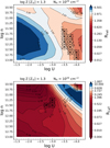 |
Fig. 3. Same as Fig. 2 but for Z ≈ 20 Z⊙ for RFeII (upper panel) and RCaT (lower panel). |
| In the text | |
|
Fig. 4. Non-monotonic behaviour of RFeII versus log UnH colour-coded with respect to log U (left panels). Corresponding cases for RCaT are shown in the right panels. The panels represent the three sets of high-metallicity cases: log Z[Z⊙]: 0 (top), 0.5 (middle), and 1 (bottom). The pale-blue vertical strip identifies the UnH product yielding the reverberation-based RBLR (black dashed line) within the uncertainties. The pale-orange horizontal strip identifies the observed RFeII and RCaT values (black dashed lines) from Persson (1988) and Marinello et al. (2016) within uncertainties. A column density of NH = 1024 cm−2 is assumed. |
| In the text | |
|
Fig. 5. Left: strength of the optical Fe II emission (RFeII) shown with respect to the distribution in cloud column density (NH) from CLOUDY. The model uses a log U = −3.5 and log n = 11.75. The colours represent nine different cases of metallicity (Z). The observed estimates from Persson (1988) and Marinello et al. (2016) for I Zw 1 are shown in cyan and orange bars (the errors in these estimates are depicted by the widths of the bars), respectively. The inset plot zooms in on a portion of the base plot to highlight the modelled trends that recover the RFeII within the observed values. We note that the RFeII is shown in log scale in the base plot while for the inset plot we show the ratio in linear scale. Right: corresponding RCaT distribution for the same modelled parameters as in the previous panel. |
| In the text | |
|
Fig. 6. Effect of microturbulence: The first and third columns are from the original models without any microturbulence for RFeII and RCaT, respectively. The second and fourth columns are the corresponding cases with microturbulence = 20 km s−1. Each column consists of the five cases of metallicity considered in this work. The overlaid symbols have the same meaning as shown previously in Fig. 2. |
| In the text | |
|
Fig. 7. Schematic view of the anisotropy in the radiation between the observer and the BLR cloud. Our model considers a simple shrinking of the radial position of the BLR to match the reverberation-mapped RBLR estimate, by filtering the incoming radiation from the accretion disc. Therefore, the net SED seen by the BLR differs from the SED seen by a distant observer. This illustration applies to I Zw 1-like sources, i.e. Type-1 Narrow-line Seyfert galaxies with high Fe II emission, which are the context of this study. |
| In the text | |
|
Fig. 8. Spectral energy distributions obtained for slim accretion discs for a representative black hole mass, MBH = 107 M⊙ for two cases of accretion rates (dimensionless): Left: |
| In the text | |
Current usage metrics show cumulative count of Article Views (full-text article views including HTML views, PDF and ePub downloads, according to the available data) and Abstracts Views on Vision4Press platform.
Data correspond to usage on the plateform after 2015. The current usage metrics is available 48-96 hours after online publication and is updated daily on week days.
Initial download of the metrics may take a while.