| Issue |
A&A
Volume 650, June 2021
|
|
|---|---|---|
| Article Number | A47 | |
| Number of page(s) | 18 | |
| Section | Stellar structure and evolution | |
| DOI | https://doi.org/10.1051/0004-6361/202040003 | |
| Published online | 07 June 2021 | |
Amplitude of solar gravity modes generated by penetrative plumes
1
STAR Institute, Université de Liège, 19C Allée du 6 Août, 4000 Liège, Belgium
e-mail: This email address is being protected from spambots. You need JavaScript enabled to view it.
2
Université Paris-Sud, Institut d’Astrophysique Spatiale, UMR 8617, CNRS, Bâtiment 121, 91405 Orsay Cedex, France
3
Observatoire de Genève, Université de Genève, 51 Ch. Des Maillettes, 1290 Sauverny, Switzerland
Received:
27
November
2020
Accepted:
3
March
2021
Abstract
Context. The observation of gravity modes is expected to give us unprecedented insights into the inner dynamics of the Sun. Nevertheless, there is currently no consensus on their detection. Within this framework, predicting their amplitudes is essential to guide future observational strategies and seismic studies.
Aims. While previous estimates considered convective turbulent eddies as the driving mechanism, our aim is to predict the amplitude of low-frequency asymptotic gravity modes generated by penetrative convection at the top of the radiative zone.
Methods. A generation model previously developed for progressive gravity waves was adapted to the case of resonant gravity modes. The stellar oscillation equations were analyzed considering the plume ram pressure at the top of the radiative zone as the forcing term. The plume velocity field was modeled in an analytical form.
Results. We obtain an analytical expression for the mode energy. It is found to depend critically on the time evolution of the plumes inside the generation region. Using a solar model, we then compute the apparent surface radial velocity of low-degree gravity modes as would be measured by the GOLF instrument, in the frequency range 10 µHz ≤ ν ≤ 100 µHz. In the case of a Gaussian plume time evolution, gravity modes turn out to be undetectable because of too small surface amplitudes. This holds true despite a wide range of values considered for the parameters of the model. In the other limiting case of an exponential time evolution, plumes are expected to drive gravity modes in a much more efficient way because of a much higher temporal coupling between the plumes and the modes than in the Gaussian case. Using reasonable values for the plume parameters based on semi-analytical models, the apparent surface velocities in this case are one order of magnitude lower than the 22-year GOLF detection threshold and lower than the previous estimates considering turbulent pressure as the driving mechanism, with a maximum value of 0.05 cm s−1 for ℓ = 1 and ν ≈ 100 µHz. When accounting for uncertainties on the plume parameters, the apparent surface velocities in the most favorable plausible case become comparable to those predicted with turbulent pressure, and the GOLF observation time required for a detection at ν ≈ 100 µHz and ℓ = 1 is reduced to about 50 yr.
Conclusions. Penetrative convection can drive gravity modes in the most favorable plausible case as efficiently as turbulent pressure, with amplitudes slightly below the current detection threshold. When detected in the future, the measurement of their amplitudes is expected to provide information on the plume dynamics at the base of the convective zone. In order to make a proper interpretation, this potential nevertheless requires further theoretical improvements in our description of penetrative plumes.
Key words: Sun: interior / hydrodynamics / stars: oscillations / asteroseismology
© ESO 2021
1. Introduction
In recent decades the study of global acoustic modes has revealed precious information on the internal properties of the Sun (see, e.g., Thompson et al. 2003; Basu & Antia 2008; Kosovichev 2011; Buldgen 2019; Christensen-Dalsgaard 2021, for interesting reviews). Among the noteworthy results, the sound speed and rotation rate could be probed with a high precision down to 0.08 R⊙ and 0.2 R⊙, respectively. Nevertheless, the study of acoustic modes hardly gives access to the properties of deeper layers, where most of the solar luminosity is produced. In contrast, gravity modes, which propagate in the central radiative zone, have the potential to probe the micro- and macrophysics inside the solar core and test further stellar models (e.g., Appourchaux et al. 2010). For instance, the detection of gravity modes, combined with neutrinos flux measurements, can be expected to improve our representation of nuclear reaction rates and electron screening (e.g., Mussack & Däppen 2011; Lopes & Turck-Chièze 2014; Bonventre & Orebi Gann 2018). The measurement of their rotational splittings can also give us the possibility to reveal the deep rotation profile and put stringent constraints on the angular momentum history of the Sun (e.g., Eggenberger et al. 2019a). From a wider perspective, all the information brought by solar gravity modes can permit, on the one hand, to calibrate stellar models and help improve our understanding of the whole stellar evolution. On the other hand, potential discrepancies between theory and observations in the earlier or later evolutionary phases can also give evidence of a change of regimes in the internal processes at work throughout the star lifetime (e.g., Gehan et al. 2018; Eggenberger et al. 2019b).
The quest for solar gravity modes began more than 40 years ago. However, gravity modes are evanescent in the convective envelope and have very small amplitudes at the solar surface; they are thus very difficult to observe. Detections have been claimed by several studies (e.g., Brookes et al. 1976; Severnyi et al. 1976; Delache & Scherrer 1983; Thomson et al. 1995; Turck-Chièze et al. 2004; García et al. 2007), but none of these results has been independently confirmed (e.g., Appourchaux & Pallé 2013). The most recent claim of their detection was made by Fossat et al. (2017) and Fossat & Schmider (2018). Using data of the GOLF instrument (e.g., Gabriel et al. 1995), the authors indirectly found evidence of the signature of low-frequency gravity modes in the time variations of the large frequency separation of high-frequency acoustic modes. Their analysis led to the identification of hundreds of gravity modes with angular degrees between ℓ = 1 and ℓ = 4, from which they could infer the asymptotic period-spacing and the mean core rotation rate. Although this work was subsequently reproduced by other studies, the robustness of the analysis was put into question (Schunker et al. 2018; Appourchaux & Corbard 2019). The result was shown to be very sensitive to the parameters of the time series considered in the analysis (e.g., the start time), and appears to be an artifact of the methodology. Theoretical studies of the coupling between acoustic and gravity modes reinforced the fragility of this result (Scherrer & Gough 2019; Böning et al. 2019). At the time of writing no robust detection of the solar gravity modes has therefore been unequivocally confirmed.
Within this framework, theoretical estimates of the amplitude of solar gravity modes are needful to help design future observational missions and guide future seismic studies. The amplitude of gravity modes results from a balance between the driving by convective motions and damping processes (e.g., Belkacem et al. 2011). Previous theoretical estimates mainly considered the Reynolds stress of turbulent convective eddies as the source mechanism, or stochastic excitation (e.g., Gough 1985; Kumar et al. 1996; Belkacem et al. 2009). Guided by global 3D numerical simulations of the solar convective zone, and using reasonable values for their model parameters, Belkacem et al. (2009) determined that the amplitudes of asymptotic gravity modes, that is, with high radial orders and oscillation frequencies between 10 µHz ≲ ν ≲ 100 µHz, are likely to lie slightly below the current GOLF detection threshold. Because of the non-detection of gravity modes, these predictions set an upper constraint on the Sun’s convective velocity in the excitation region (around 0.8 R⊙). However, all these previous estimates did not account for the contribution from the penetration of convective plumes at the base of the convective region (or penetrative convection) to the mode driving.
Convective plumes are strong downdrafts originating from diving cool granules at the solar surface. They develop by turbulent entrainment of matter as coherent structures when crossing the convective region (e.g., Turner 1986; Rieutord & Zahn 1995). As the plumes reach the bottom of the convective bulk, they can penetrate into the underlying stably stratified radiative layers; there the plumes are braked by buoyancy and can transfer a part of their kinetic energy into gravity waves. While this excitation mechanism is ubiquitous in numerical simulations of extended convective envelopes overlying radiative zones (e.g., Andersen 1996; Dintrans et al. 2005; Kiraga et al. 2005; Rogers et al. 2006, 2013; Alvan et al. 2014; Edelmann et al. 2019), the covered values of the dimensionless control parameters are far from stellar regimes. Quantitative estimates by means of semi-analytical excitation models are thus required and complementary (e.g., Rempel 2004). Motivated by the issue of the redistribution of angular momentum in stellar interiors, Pinçon et al. (2016) modeled this driving process to predict the amplitude of very low-frequency progressive gravity waves propagating in the radiative zone of the Sun. They demonstrated that this process generates low-frequency gravity waves more efficiently than turbulent pressure and can have an important impact on the angular momentum evolution of low-mass stars (Pinçon et al. 2017). However, no application regarding the amplitude of the solar gravity modes with much higher frequencies has been undertaken so far.
In this work we estimate the amplitude of the solar gravity modes generated by penetrative convection following the model of Pinçon et al. (2016). We limit the study to asymptotic gravity modes in the frequency range between 10 µHz and 100 µHz (i.e., with a number of radial nodes much higher than unity). The damping of such modes is dominated by radiative losses, and is analytically tractable in the considered frequency range under the quasi-adiabatic limit (e.g., Dziembowski 1977b; Belkacem et al. 2009). In contrast, at higher frequencies the computation of the mode damping requires accounting for the interaction between oscillations and convection, which is much more complex and beyond the scope of this paper (e.g., Belkacem et al. 2011).
The paper is organized as follows. In Sect. 2, an analytical expression for the mode energy is derived based on the model of Pinçon et al. (2016). In Sect. 3 the apparent surface radial velocity of gravity modes is estimated from this expression for a solar model and is compared to the GOLF data detection threshold. The results are discussed in Sect. 4. The conclusions are presented in Sect. 5.
2. Excitation model by penetrative convection
In this section we derive an analytical expression for the energy of gravity modes excited by penetrative convection. The asymptotic (i.e., short-wavelength) approximation is used and the quasi-adiabatic limit is considered (i.e., non-adiabatic effects are globally considered as small perturbations). Both approximations are justified for the Sun in the considered frequency range (between 10 µHz and 100 µHz). The detailed derivation steps and technical issues are described in Appendix A.
2.1. Oscillation equations forced by penetrative plumes
Following Pinçon et al. (2016), the velocity field in the stellar frame is decomposed into a component associated with the convective plumes and a perturbation associated with the gravity modes. The source term in the linearized momentum equation is assumed to be the ram pressure exerted by the ensemble of convective plumes at the top of the radiative region. The feedback from the oscillations on the plume structure and dynamics is neglected. In other words, we assume that the wave energy is much lower than the plume kinetic energy at the base of the convection zone, which is checked a posteriori. The effect of the Coriolis force on both the oscillations and the plumes is not considered. This is justified for the gravity modes as the solar rotation period is much shorter than the modal periods. For the plumes, the effect of the buoyancy work is predominant so that the plume Rossby number is expected to be very low in the case of slow rotators as the Sun.
Within this framework, the forced linear non-adiabatic oscillation equation reads (see Appendix A.1 for details)
 (1)
(1)
where ξ(r, t) is the mode displacement field, H is the temperature scale height, δS is the Lagrangian perturbation of specific entropy, cp is the specific heat capacity at constant pressure, ρ is the equilibrium density, 𝒱p(r, t) is the velocity field associated with the ensemble of plumes, ℒad is the adiabatic differential operator provided in Eq. (A.7), ℒnad is a differential operator given in Eq. (A.6) and resulting from non-adiabatic effects, ∂t denotes the partial time derivative, ∇ is the gradient operator, and (⊗) is the outer product.
Monitoring the evolution of δS requires us to consider the perturbed heat equation. Accounting only for radiative losses in the case of asymptotic gravity modes, the perturbed heat equation can be expressed within the diffusion approximation as (see Appendix A.2.1)
![Mathematical equation: $$ \begin{aligned} \partial _t \left( \frac{\delta S}{c_p} \right)=\frac{1}{t_{\rm R}} \left[ \mathcal{L} ^{\mathrm{nad}1}\left( \frac{\boldsymbol{\xi }}{H}\right)+\mathcal{L} ^{\mathrm{nad}2} \left( \frac{\delta S}{c_p}\right)\right] , \end{aligned} $$](/articles/aa/full_html/2021/06/aa40003-20/aa40003-20-eq2.gif) (2)
(2)
where tR = ρcpTH/FR is the local radiative thermal timescale, which describes the exchange rate of energy between the modes and the radiation, with FR and T the equilibrium radiative flux and temperature, respectively. We note that ℒnad1 and ℒnad2 in this equation are dimensionless linear differential operators with respect to radius and represent the perturbation of the divergence of the radiative flux. We also note that tR is equal to the local thermal timescale in the radiative zone and in a very thin near-surface layer where the energy flux is mostly carried by radiation. This is not the case in deeper convective layers where the energy flux is mostly carried by the convective flux, but whose influence on the considered gravity modes can be neglected according to the numerical computations of Belkacem et al. (2009).
2.2. Mode amplitude in the quasi-adiabatic limit
2.2.1. Decomposition on the adiabatic eigenfunction basis
The eigenfunctions ξnℓm of the ℒad operator, with radial orders n, angular degrees ℓ, and azimuthal numbers m, were shown to form a complete basis of the oscillation displacement field under the zero-boundary conditions (e.g., Chandrasekhar 1964; Unno et al. 1989). More precisely, the demonstration relied on the assumption that the oscillations are adiabatic (i.e., δS = 0). For our purpose we show in Appendix B that they also form a complete basis of the oscillation displacement field in the non-adiabatic case (i.e., δS ≠ 0). It is therefore possible to project the non-adiabatic mode displacement field onto the basis of the eigenfunctions of the ℒad operator. This gives
 (3)
(3)
where we have introduced the instantaneous amplitude anℓm. The eigenfunctions satisfy the eigenvalue relation
 (4)
(4)
with
 (5)
(5)
where ωnℓm is the angular eigenfrequency; (r, θ, φ) are the spherical coordinates in the stellar frame;  and
and  are the (real) radial and poloidal components of the eigenfunctions, respectively, which are normalized such as
  = 1 at the photosphere; and
  are the orthonormal spherical harmonics. The eigenfunctions are orthogonal with respect to the density-weighted inner product and their mode mass is defined as
 (6)
(6)
where V is the stellar volume beyond which the stellar density vanishes and (⋆) denotes the complex conjugate.
2.2.2. Globally quasi-adiabatic gravity modes
Asymptotic gravity modes are incompressible (e.g., Dintrans & Rieutord 2001), so that ℒnad1 and ℒnad2 in Eq. (2) are dominated by second-order derivatives with respect to radius, and their local norms scale as  when applied on a harmonic (n, ℓ, m), where λnℓm(r) is the local radial wavelength (see Appendix A.2.2). Consequently, the time evolution of the amplitude anℓm is simultaneously governed by the local damping timescale given by
  in Eq. (2) and the dynamical timescale tdyn ∼ 1/ωnℓm in Eq. (1). Almost everywhere in the star the quasi-adiabatic limit is supposed to be met, that is,
 (7)
(7)
and the non-adiabatic effects represented by the quantity δS/cp can be locally treated as a small perturbation (e.g., Dziembowski 1977b). This is not met in a very thin near-surface layer where the density vanishes and tR, which is equivalent to the thermal timescale in this region, becomes much smaller than dynamical timescale (see, e.g., Fig. 2b in Berthomieu & Provost 1990). However, this region is so thin and the part of the total mode energy contained inside is so small that its impact on the global mode damping is expected to be negligible. This expectation is again supported by the numerical computations of Belkacem et al. (2009), who demonstrated that the work performed by the radiative flux variations on the oscillations mainly originates from the radiative cavity for the considered frequency range.
In order to reason in a global way we therefore define a global damping timescale, denoted Tdamp, which aims to measure the impact of the non-adiabatic effects on the global behavior of a harmonic (n, ℓ, m). Owing to the place of tdamp in Eq. (2), Tdamp is taken equal to the inverse of the harmonic mean of 1/tdamp(r) weighted by the local mode energy. Considering only the contribution from the radiative zone to the mode damping, Tdamp reduces to Eq. (A.54) in the asymptotic frequency range, that is,
 (8)
(8)
where rb denotes the radius of the base of the convective zone. In the following, we thus assume that the oscillations are globally quasi-adiabatic in the considered frequency range:
 (9)
(9)
The definition in Eq. (8) appears to be relevant and eases the computation of the mode amplitude.
2.2.3. Forced amplitude
Projecting Eq. (1) on ξnℓm and expressing δS by means of Eq. (2), a set of coupled third-order linear differential equations for the dependent variables anℓm(t) can then be obtained, each of them accounting for the first-order non-adiabatic perturbations (see Appendix A.2.3). These equations involve a fast timescale, which is tdyn, and a slow timescale, which is actually Tdamp defined in Eq. (8). It thus appears judicious to solve the differential system using a two-timing method (e.g., Kevorkian 1961). This method can provide us with a uniformly valid solution up to timescales on the order of Tdamp. A two-timing analysis is sufficient for the present purpose since most of the mode energy is dissipated on a timescale on the order of Tdamp, so that the error made is expected to be small compared to other uncertainties related, for instance, to the modeling of the generation process.
Expressing explicitly the partial derivatives with respect to the fast and slow timescales in the amplitude equations, and grouping together the terms of the same order, a two-timing approach ultimately leads to the mode amplitude (see Appendix A.2.4)
 (10)
(10)
with
 (11)
(11)
where  is provided by Eq. (A.27). This term results from the scalar projection of the plume driving term in Eq. (1) on ξnℓm normalized by the mode mass. In addition, the expression of the damping rate ηnℓm is compatible, within the asymptotic limit, with the usual quasi-adiabatic expression provided, for example, by Dziembowski et al. (2001) or Godart et al. (2009). Its expression is provided in Eqs. (A.59) and (A.60) from which we deduce that ηnℓm ∼ 1/Tdamp. This confirms a posteriori our choice for the definition of the global damping timescale in Eq. (8).
At this point we note that Eq. (10) can be retrieved if we assume that the solutions of the homogeneous equations for each amplitude anℓm take the form of an exponentially damped harmonic oscillator, as usually done in quasi-adiabatic analyses (e.g., Dziembowski 1977b; Unno et al. 1989), and then use this ansatz to find the particular solution of the forced equations. Nevertheless, the present analysis also clearly highlights two essential points. First, Eq. (10) is uniformly valid up to a timescale on the order of Tdamp only. Second, it appears that Eq. (10) holds true if the coupling induced by the ℒnad operator in Eq. (1) between the different (n, ℓ, m) components remains negligible. Assuming that modes with adjacent radial orders n and n + 1 have comparable amplitudes for given values of ℓ and m, this is met if we have (see Appendix A.2.4)
 (12)
(12)
where Δtcore is the time spent by a wave energy ray of frequency ωnℓm to cross the radiative core. In this case the radiative losses accumulated during a one-travel path of a wave through the radiative core are negligible; as a result, the resonant modes keep at leading order the same global structure as the eigenfunctions of ℒad, except for the small exponential decay of their amplitudes with time (see discussion in Appendix A.2.4). We show in Sect. 3 that this is met for a solar model in the considered frequency range. The relative error made when writing Eq. (10) thus turns out to be on the order of Δtcore/Tdamp at most.
To express further Eq. (10) we need to model the  term, and thus to specify the plume velocity field.
2.3. Modeling the plumes and the penetration zone
While the mean ensemble behavior of convective plumes has been widely studied in numerical simulations, for example, how they structure together, how they can merge, or how efficiently they can transport energy (e.g., von Hardenberg et al. 2008; Pieri et al. 2016; Pratt et al. 2017), to the authors’ knowledge there is no quantitative description of their detailed structures. Moreover, though useful to guide the investigations, the outcomes of the current numerical simulations of extended convective envelopes still have to be taken with caution (e.g., Rempel 2004).
In the present work we thus choose to follow an analytical description based on the model of Pinçon et al. (2016). The penetration of convective plumes is supposed to be a random, stationary, and ergodic process. We assume that, on average, 𝒩 identical plumes (i.e., with the same velocity and shape) are penetrating at each time and can transfer their energy into gravity modes. The plumes are supposed to be incoherent with each other and uniformly distributed on the sphere. At the base of the convective region, the Péclet number, which represents the ratio of the efficiency of the advection of heat by the plumes to the efficiency of the radiative diffusion, is expected to be much larger than unity in the Sun (see Sect. 3.2). As a result, the convective plumes are braked over a very small penetration length (i.e., relative to the local pressure scale height) below the radius where the Schwarzschild criterion is met (Zahn 1991; Dintrans et al. 2005). The plume ram pressure gradient is thus supposed to be maximum inside the penetration region, and to vanish outside. The analytical form of the velocity field inside the penetration region that is associated with a plume penetrating at t = 0 and whose center has for latitudinal and azimuthal coordinates (θ0, φ0) reads (Pinçon et al. 2016, cf. Eqs. (19) and (20))
 (13)
(13)
where the f function represents the time evolution of the plume velocity, with τp the plume lifetime, 𝒱r is the radial profile, b is the plume radius, and Sh(r; θ0, φ0) corresponds to the distance on a concentric sphere from the center of the plume.
Owing to the large Péclet number, an adiabatic temperature gradient is imposed in the penetration zone; 𝒱r can thus follow the model of penetrative convection of Zahn (1991). The value of the plume velocity at the entry of the penetration region, denoted Vb, and that of the radius b are adapted from the model of turbulent plumes developed by Rieutord & Zahn (1995). Below this region, the transition from an adiabatic to a radiative temperature gradient is supposed to be very sharp, so that the Brunt-Väisälä frequency discontinuously changes from about zero in the adiabatic region to Nt at the top of the radiative zone. We note that this hypothesis is supported by the recent seismic inversions of the Brunt-Väisälä frequency in the Sun performed by Buldgen et al. (2020). Their observations show that the transition from an adiabatic to a radiative gradient at the base of the convective zone occurs over a distance dtrans representing about 0.5% of the solar radius and that the value of Nt is equal to about 550 µHz. As a result, we find that dtrans is much smaller than the local wavelength in the considered ranges of frequencies and degrees. This justifies the fact that, from the point of view of the gravity modes, the profile of the Brunt-Väisälä frequency can be supposed to be discontinuous at the top of the radiative zone.
Finally, the time evolution of the plumes in the penetration region is badly understood. Pinçon et al. (2016) identified two probable plume destruction processes: baroclinic instabilities and turbulence. Using orders of magnitude, they estimated that the plume lifetime is most likely in the range around the convective turnover timescale of turbulent eddies at the base of the convective region, τconv. Regarding the profile, they assumed that the penetration of a plume is a short-lived event and follows a Gaussian law in time, as in the initial work of Townsend (1966). Nevertheless, given the related uncertainties, it is relevant to test other prescriptions. Within the framework of the stochastic excitation of gravity modes, the spectral density of turbulent kinetic energy of convective eddies was also usually assumed to be Gaussian until Belkacem et al. (2009), based on 3D numerical simulations, showed that a Lorentzian form is more appropriate. Gaussian and Lorentzian laws represent two limiting cases in the time Fourier domain, since they stand for very rapidly and very slowly decreasing functions of frequency, respectively. By analogy, the spectral density of kinetic energy of the plumes will be also supposed to be Lorentzian, which, in the time domain, is equivalent to assuming an exponential time profile. Therefore, the f(t) function in Eq. (13) will be equal in the two limiting cases to either
 (14)
(14)
2.4. Mean mode energy
Owing to the random properties of the generation process, a statistical approach has to be considered. As the time-averaged mode amplitude vanishes, we need to estimate either the mean mode square amplitude or the mean mode energy. We find it more appropriate to reason in a first step on the mean mode energy since it does not depend on the chosen normalization of the eigenfunction basis, whereas the amplitude does. Because of the incoherence between the convective plumes, we first note that the wave velocity fields generated by different plumes cancel each other out. Assuming in addition that excitation is a stationary process and the plumes are all identical and uniformly distributed over the sphere, we show in Appendix A.3.1 that the total mean mode energy is merely equal to the oscillation energy generated by one single plume penetrating at t = 0 and averaged over its angular position (θ0, φ0), multiplied by the instantaneous number of penetrating plumes 𝒩. Therefore, using Eq. (13) in Eq. (10), it is possible to compute the mean oscillation energy associated with each orthogonal (n, ℓ, m) harmonic. In the asymptotic limit, the WKB form of the eigenfunctions can be used to formulate the result analytically (see Appendix A.3.2). In the case of a large Péclet number at the base of the convective region, that is, for a very small penetration region, we find that the mean energy of the (n, ℓ, m) harmonic can be finally expressed as (see Appendix A.3.5)
![Mathematical equation: $$ \begin{aligned} \langle E_{n\ell m} \rangle \approx \dfrac{ \left[(\omega _{n\ell m} \Delta \Pi _\ell /\pi ^2)\ \overline{L_{\rm p}}\ F_{\mathrm{d},\ell } \ e^{-\ell (\ell +1) b^2/2 r_{\rm b}^2} \ \mathcal{C} _{n\ell m}\right]}{2\eta _{n\ell m}} , \end{aligned} $$](/articles/aa/full_html/2021/06/aa40003-20/aa40003-20-eq23.gif) (15)
(15)
with
 (16)
(16)
where ΔΠℓ is the asymptotic period spacing between two consecutive adiabatic gravity modes of degree ℓ given in Eq. (A.39),  is the mean plume kinetic luminosity through the shell of radius rb at the base of the convective zone,
  is the plume filling factor, 𝒮p = πb2 is the area occupied by a single plume, ρb and Vb represent the density and the plume velocity at rb, and Fd, ℓ = Vbkh, b/Nt is the Froude number at the top of the radiative zone, with
  the horizontal wavenumber of the mode.
We note that the numerator of Eq. (15) represents the amount of power injected into the mode per unit of time. The term inside the brackets refers to the mode mass. The Gaussian term represents the horizontal correlation between the plumes and the mode, while 𝒞nℓm measures the temporal correlation. The general analytical expression of 𝒞nℓm is provided by either Eq. (A.56) in the case of a Gaussian plume time evolution (i.e., f = fG) or Eq. (A.55) in the case of an exponential plume time evolution (i.e., f = fE). In the considered frequency range we usually have ηnℓm ≪ νp ≪ ωnℓm, where νp = 1/τp. As a result, 𝒞nℓm is merely equal to (see Appendix A.3.3)
 (17)
(17)
and
 (18)
(18)
In the considered frequency range, the temporal correlation is thus expected to be much smaller in the Gaussian case than in the exponential case; as a result, the mean mode energy is also expected to be smaller. This will be discussed in greater detail in Sect. 3.
Moreover, within the quasi-adiabatic and asymptotic limits  , as shown by Eq. (A.60) and illustrated in Fig. 1 (e.g., Godart et al. 2009). In the considered frequency range Eqs. (15)–(18) thus demonstrate that ⟨Enℓm⟩ is independent of the frequency when f = fE, whereas ⟨Enℓm⟩ is inversely proportional to the squared frequency when f = fG. In both cases the mean mode energy decreases as ℓ increases. As in the case of low-frequency progressive internal gravity waves, we see according to Eq. (15) that the excitation efficiency is mainly measured by the Froude number at the top of the radiative region, which is expected to be much smaller than unity in stars (see Sect. 3.1). As the correlation and mode mass terms are also smaller than unity, the mean mode energy turns out to be much smaller than the mean plume kinetic energy at the base of the convective zone, and we check a posteriori that the feedback from the modes to the plume dynamics inside the penetration region is negligible.
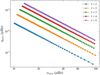 |
Fig. 1. Radiative damping rate as a function of the oscillation frequency νnℓm and the angular degree ℓ. Each circle corresponds to a given eigenmode. |
2.5. Apparent mode radial velocity
Owing to a high signal-to-noise ratio, the search for the solar gravity modes is usually performed through radial velocity measurements integrated over the full solar disk (e.g., Appourchaux et al. 2010). In order to be compared to the observed measurements, the theoretical mean mode energy has to be converted into mean mode radial velocity accounting for the line-of-sight projection and the limb-darkening effects (Dziembowski 1977a; Berthomieu & Provost 1990). Among other observational effects that need to be corrected, they are expected to be the predominant ones. Following the computation of Belkacem et al. (2009), we show in Appendix C that the mean apparent radial mode velocity for a (n, ℓ, m) harmonic is equal, in the slow rotator limit, to
 (19)
(19)
where  is identified as
 (20)
(20)
with rabs the radius in the atmosphere where the absorption line considered to measure the radial velocity is formed. The visibility coefficients  and
and  are provided in Eqs. (C.6) and (C.7). They depend on the limb-darkening law and on the angle between the stellar rotation axis and the line of sight.
We note that, contrary to the mode energy, it is not possible to express Eq. (20) using the WKB form of the eigenfunctions as it becomes questionable in the convective region and the atmosphere of stars. The estimate of Eq. (20) therefore requires the numerical computation of the mode eigenfunctions and their mode masses.
3. Applications to gravity modes in the Sun
In this section the excitation model is used to predict the apparent surface radial velocity of gravity modes generated by penetrative convection for a solar model. As in Belkacem et al. (2009), we choose to compare our results to the detection threshold of the GOLF instrument on board the SoHO spacecraft (e.g., Gabriel et al. 1995).
3.1. Solar model
We consider a calibrated solar model computed with the stellar evolution code CESTAM (Marques et al. 2013). The chemical composition follows the solar mixture, as given in Asplund et al. (2009), with initial helium and metal abundances Y0 = 0.25 and Z0 = 0.013. The OPAL 2005 equation of states and opacity tables as well as the NACRE nuclear reaction rates were used to build the model. The atmosphere was constructed following an Eddington gray approximation, and convection was modeled using the mixing-length theory with a parameter αMLT = 1.62. Microscopic diffusion, overshooting, and rotation were not taken into account. We note that the obtained solar structure, although imprecise from the point of view of seismic inversions, is sufficient for our purpose as the uncertainties related to the assumptions considered in the excitation model are dominant. For example, it is known that microscopic diffusion can slightly modify the stratification at the base of the convective zone (e.g., Christensen-Dalsgaard et al. 1993) and hence can affect the properties of the penetrating plumes. Nevertheless, this effect is expected to be much smaller than the uncertainties related, for instance, to the plume formation mechanism across the convection zone.
The adiabatic eigenfrequencies νnℓm = ωnℓm/2π, eigenfunctions, and mode masses needed to compute Eq. (19) were obtained via the oscillation code ADIPLS (Christensen-Dalsgaard 2008). The eigenfunctions were normalized such that  = 1 at the photosphere. Owing to the large drop in the density and pressure at the stellar surface, the reflective zero-boundary conditions are considered. We check that the period spacing between consecutive ℓ = 1 eigenmodes is very close to the asymptotic value, that is, ΔΠℓ = 1 ≈ 26 min. Moreover, the mode mass is nearly proportional to ℓ3 and
  (see, e.g., Fig. 6 in Belkacem et al. 2009). To be complete, the radiative damping rate occurring in Eq. (15) and computed according to the quasi-adiabatic expression provided in Eq. (A.60) is plotted in Fig. 1. In this figure, we first see that the damping rate is very similar to that computed numerically by Belkacem et al. (2009, see Fig. 9) who also accounted for the influence of the upper layers. This confirms our assumption that the work performed in the inner radiative cavity is the main contributor to the damping of the asymptotic gravity modes. Second, we also see in this figure that the damping timescale Tdamp ∼ 1/ηnℓm is more than six orders of magnitude higher than the oscillation timescale tdyn ∼ 1/ωnℓm. This justifies a posteriori the use of the global quasi-adiabatic approximation in this frequency range. Moreover, since n ≲ 103 in the considered frequency range, it is obvious that Δtcore ≈ ntdyn ≪ Tdamp, so that the hypothesis made in Eq. (12) appears a posteriori to be valid as well (i.e., the coupling induced by non-adiabatic effects between adjacent radial orders is negligible up to a timescale on the order of Tdamp).
3.2. GOLF apparent radial velocity with standard parameters
The internal structure of the solar model provides us with all the equilibrium quantities to compute the parameters of the excitation model and the mode apparent velocity in Eq. (19). The radius at the base of the convective zone and the local density are equal to rb ≈ 5.2 105 km and ρb ≈ 125 kg m−3. Based on the model of plumes of Rieutord & Zahn (1995), we find b ≈ 104 km and Vb ≈ 190 m s−1. The Péclet number at the base of the convective region is estimated to be about equal to VbH(rb)/Krad(rb)∼107, where H and Krad are the temperature scale height and the radiative diffusivity, respectively. The large Péclet number assumption used in Sect. 2.3 is thus justified for the Sun. Following Buldgen et al. (2020), the Brunt-Väisälä frequency just below rb is taken equal to Nt = 550 µHz. The Froude number at the top of the radiative zone is thus equal to Fd, 1 ≈ 10−3. Moreover, we use a reasonable value 𝒩 ≈ 1000, as previously estimated by Rieutord & Zahn (1995), which corresponds to 𝒜 ≈ 0.08, in qualitative agreement with previous numerical simulations (e.g., Stein & Nordlund 1998; Brummell et al. 2002). The convective turnover timescale at the base of the convective region is equal to about τconv ≈ 10 days according to the convection mixing length theory, which leads to νp ≈ 1/τconv ≈ 1 µHz. At this point, the considered values of the plume parameters are referred to as the standard values. We consider that the sodium NaD1 and NaD2 absorption lines used by the GOLF instrument to measure radial velocities at height h ≈ 300km above the photosphere (Bruls & Rutten 1992). We also use the limb-darkening law as formulated by Ulrich et al. (2000), and take for the angle between the stellar rotation axis and the line of sight Θ0 ≈ 83°. Moreover, we systematically focus on the azimuthal numbers |m|=ℓ in what follows as we find they are less attenuated by the visibility effects and we want to study the more optimistic case.
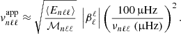
Using all these physical ingredients, we can compute the apparent radial velocity of the asymptotic gravity modes,  , between 10 µHz and 100 µHz. The result is plotted in Fig. 2 as a function of the mode eigenfrequencies and for typical degrees ℓ = 1−5. Both limiting cases of a Gaussian and exponential plume time evolution are considered and compared.
 |
Fig. 2. Apparent surface radial velocity of solar gravity modes as a function of the oscillation frequency νnℓm and the angular degree ℓ, for azimuthal numbers m = ℓ and for standard plume parameters. The results obtained with a Gaussian and an exponential plume time evolution (see Sect. 2.3) are represented by the diamonds and the plus signs, respectively, for each considered eigenmode. The thick dashed gray line corresponds to the 22-year GOLF detection threshold (see Sect. 3.3). The blue dash-dotted line represents the upper limit for the amplitude of the dipolar modes when accounting for the largest plausible variations in the plume parameters (i.e., with a factor of two increase in the inverse plume lifetime and radius; see Sect. 4.3). |
First, Fig. 2 shows in both cases that the apparent surface velocity of the gravity modes generated by penetrative convection is maximum for ℓ = 1 and sharply drops as a function of ℓ. At a given frequency, the difference of apparent velocity between the ℓ = 1 and ℓ = 5 modes is larger than about two orders of magnitude. In addition,  appears to depend linearly on the frequency in the exponential case, while it is almost independent of frequency in the Gaussian case. In order to disentangle the reasons for such trends from the different terms occurring in Eq. (19), we propose to rewrite Eq. (20) in a more simple way. Owing to the reflective boundary conditions, the Lagrangian perturbation of pressure vanishes at the solar surface, which leads to (e.g., Unno et al. 1989)
 (21)
(21)
where G is the gravitation constant, M⊙ and R⊙ are the solar mass and radius, and where we considered the normalization  . Therefore, over the considered frequency range, we have
  . Moreover, we can assume that
  does not significantly vary in the solar atmosphere, that is,
  . We checked the validity of this approximation using the numerical eigenfunctions. Since
  is approximately equal to or smaller than
  (see Table 1), Eq. (19) can thus be expressed at first approximation as
 (22)
(22)
Absolute values of the visibility factors of the GOLF instrument as a function of the angular degree ℓ.
For ℓ = 1−5, the Gaussian term in Eq. (15) remains close to unity since ℓ ≪ rb/b ∼ 50. As a consequence, since 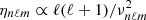 , we find according to Sect. 2.4 that
  in the Gaussian case and ⟨Enℓm⟩∝ℓ−2 in the exponential case. In addition, as the mode mass depends approximately on νnℓm and ℓ as
  , Eq. (22) leads in the Gaussian case to
 (23)
(23)
and in the exponential case to
 (24)
(24)
As shown in Table 1, the value of  smoothly varies with ℓ, and the trends predicted in Eqs. (23) and (24) are in qualitative agreement with Fig. 2. It thus appears that the simultaneous influence of the mode mass and the damping rate counterbalances the decrease in the mode driving with frequency (via the temporal correlation term). This explains the trends observed in Fig. 2.
Moreover, we clearly show in Fig. 2 that the value of  predicted assuming a Gaussian plume time evolution at a given ℓ is at least three orders of magnitude smaller than that assuming an exponential plume time evolution. This huge difference results from the much smaller temporal correlation between the plumes and the considered eigenmodes in case of a Gaussian time evolution, which is represented by the 𝒞nℓm term. In this case the spectral density of the plume kinetic energy is mostly carried by the frequencies lower than νp. As νnℓm ≫ νp, the coupling between the plumes and the eigenmodes is very small, and the excitation is very inefficient. In contrast, in the case of an exponential time evolution, the spectral density of the plume kinetic energy is distributed over higher frequencies, and the coupling between the plumes and the eigenmodes is maximum for frequencies around νnℓm (see the computation in Appendix A.3.3). As a result, the energy transfer from the plumes to the modes is much more efficient. Considering Eqs. (17) and (18) in Eqs. (15) and (19), the ratio of the mode apparent velocity in the Gaussian case to that in the exponential case scales as
  . Since
  in the quasi-adiabatic limit, this ratio is expected to decrease as 1/νnℓm, in agreement with Fig. 2. Our estimate therefore demonstrates that the amplitude of the asymptotic solar gravity modes generated by penetrative convection critically depends on the plume time evolution at the base of the convective zone. Our lack of knowledge on the plume dynamics in this region thus prevents us from quantitatively predicting the efficiency of this excitation process. In turn, if detected, solar gravity modes can be expected to put important constraints on penetrative convection at the top of the radiative zone (see discussion in Sect. 4.4).
Finally, we point out that over the considered frequency range the GOLF apparent radial velocity of the gravity modes computed with the present model and standard plume parameters is about one order of magnitude smaller than that predicted considering turbulent pressure as the driving mechanism. For the ℓ = 1 modes in the exponential case, for which the excitation is the most efficient, our predictions lie between  cm s−1 from νnℓm = 10 µHz to νnℓm = 100 µHz, while those of Belkacem et al. (2009) lie between
  m s−1 (see Sect. 4.2 for a more detailed comparison). These results therefore suggest that penetrative convection is less efficient than turbulent convection to generate asymptotic gravity modes in the Sun. Nevertheless, owing to a significant sensitivity of the predictions to the plume parameters (i.e., velocity, radius, lifetime), whose values are currently affected by uncertainties, we note that reasonable variations in these parameters are likely to reduce the gap between the two excitation mechanisms (see blue dash-dotted line in Fig. 2). This point is discussed further in Sect. 4.3.
3.3. Comparison with the GOLF detection threshold
Using a statistical approach, Appourchaux et al. (2010) could analytically express the threshold signal-to-noise ratio above which a peak in the power spectral density (PSD) of an observed time series can be considered as a relevant oscillating signal over a frequency interval Δf, with a false alarm probability pth that the measurement is due to pure noise. As shown in Appendix D, this threshold can be converted into a detection threshold for the root mean square oscillation velocity, denoted with vth, above which a signal would be detected with a certain confidence level. It reads
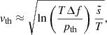 (25)
(25)
where T is the observation time and  is the mean noise level in the PSD over the range Δf.
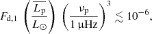
We consider a GOLF observation time equal to T = 22 yr. The mean noise level  is estimated from García et al. (2007, see Appendix D). We choose Δf = 10 µHz and pth = 0.01. Instead of a common rejection level of 10%, we adopt a rejection level of 1% since it allows the posterior probability that a peak is due to noise to reach lower values close to 10%, as already mentioned in Appourchaux et al. (2010). The resulting 22-year GOLF detection threshold is represented by a thick gray dashed line in Fig. 2. We see that the threshold velocity smoothly decreases from about 1 cm s−1 at νnℓm = 10 µHz to about 0.5 cm s−1 at νnℓm = 100 µHz. This trend results from the decrease in the solar granulation noise with frequency in the GOLF data. Its value is about five orders of magnitude higher than the apparent mode velocity throughout the considered frequency range when assuming a Gaussian plume time evolution. According to Eq. (25) the amplitude of gravity modes will be lower even if the observation time is equal to ten billion years. In the case of an exponential plume time evolution, the amplitude predicted with standard plume parameters is also at least one order of magnitude lower than the 22-year GOLF detection threshold over the considered frequency range. Based on our simple estimate of the GOLF mean noise level (see Eq. (D.2)), Eq. (25) requires an unreachable GOLF observation time T ∼ 2000 yr to detect the dipolar n = 6 gravity mode at νnℓm ≈ 90 µHz. In conclusion, using standard values for the plume parameters, our model indicates that the solar asymptotic gravity modes generated by penetrative convection remains far from being detected in an acceptable observation time by radial velocity measurements such as performed by the GOLF instrument. It is worth mentioning that the uncertainties on the predicted amplitude, which are inherent to uncertainties on the plume parameters, may nevertheless considerably reduce the observation time required for a reliable detection. This potential is also evaluated in Sect. 4.3.
4. Discussion
4.1. Comparison with the estimate of Andersen (1996)
Andersen (1996) first investigated the generation of solar gravity modes by penetrative convection using both numerical simulations and simple energy considerations. Including an ad hoc forcing term at the top of the radiative region that mimics the influence of penetrative plumes in a solar model, he numerically solved the wave equations and computed the transmission of the generated wave energy throughout the convective envelope, the structure of which was taken from the turbulent numerical simulations of Andersen (1994). He found that the wave transmission up to the surface is on the order of 0.05%. Using these results, he could estimate that the horizontal velocity of gravity modes near the solar surface ranges between 0.01−1 mm s−1 for ℓ = 6 and νnℓm = 50−100 µHz. When accounting for an appropriate GOLF visibility factor, that is  , this upper value turns out to be much larger than our predictions in the case of a Gaussian plume time evolution, but on the same order of magnitude in the exponential case. However, we note that this qualitative agreement is more likely to be fortuitous. In order to estimate the amplitude of gravity modes, Andersen (1996) assumed that the total mode energy is equal to the part of the convective kinetic energy transferred on average to progressive gravity waves in the numerical simulation of Andersen (1994), the upper and lower boundary conditions of which are open. As a consequence, this estimate actually did not properly account for the quasi-stationarity of the modes or for the damping processes. Therefore, although qualitatively comparable for the ℓ = 6 gravity modes, the physical origins of our predictions radically differ from those of Andersen (1996), and drawing conclusions from their comparison ultimately appears irrelevant.
4.2. Comparison with turbulence-induced gravity modes
Belkacem et al. (2009) modeled the generation of asymptotic gravity modes by considering the turbulent Reynolds stress as the driving mechanism. As mentioned at the end of Sect. 3.2, the surface mode velocity they predicted is one order of magnitude higher than our estimate in the exponential case when considering standard values for the plume parameters based on semi-analytical models and orders of magnitude. Nevertheless, for both excitation mechanisms, the dependence of the apparent radial velocities on ℓ and νnℓm turns out to be comparable (e.g., Belkacem et al. 2009, see Fig. 11). This similar dependence results on the one hand from the mode mass and the damping rate, which play the same role in both excitation processes, and on the other hand from a comparable temporal correlation between the driving source and the modes. Belkacem et al. (2009) assumed that the time coherence of the convective eddies is exponential; as a result, the temporal correlation between the modes and the eddies has a similar form to that between the modes and the plumes when assuming an exponential plume time profile (e.g., a dependence on about  ; see Eqs. (1)–(2) and Fig. 3 in Belkacem et al. 2009). Regarding the magnitude, as the velocity of the turbulent eddies that drive gravity modes is about equal to vMLT ≈ 60 m s−1 (according to the mixing length theory), which is about three times lower than the plume velocity at the base of the convective zone, penetrative convection could have been at first sight expected to generate gravity modes with higher amplitudes. However, while the excitation by penetrative convection occurs in a very thin shell at the base of the convective zone, convective eddies can drive gravity modes in a larger volume of the envelope. Moreover, as the eddy turnover frequencies are higher than νp in the upper layers of the convective region, the time correlation is larger for the excitation by turbulent convection than by penetrative plumes. The lower velocities of the convective eddies are thus compensated by a more extended excitation region and a better temporal correlation with the modes, leading to higher amplitudes in the exponential case.
In contrast, when assuming that the eddy-time coherence is Gaussian, as in Kumar et al. (1996), Belkacem et al. (2009) found the apparent radial velocities of gravity modes generated by turbulent eddies is on the order of 10−3 cm s−1. Although their predictions also depend on νnℓm and ℓ in a similar way to our predictions in the Gaussian case, their magnitude is much larger than ours. While the same arguments as in the previous paragraph hold true to explain the similarities in the dependence on νnℓm and ℓ, the temporal correlation with the modes in the Gaussian case is very sensitive to the timescales associated with the driving source. As the values of the turnover frequencies of the turbulent eddies driving the modes are larger than νp, the temporal correlation is expected to be much larger than for the excitation by plumes. This certainly explains the huge difference between the excitation by turbulent convection and penetrative convection in the Gaussian case.
4.3. Sensitivity of the mode amplitude to the plume parameters
As shown by Pinçon et al. (2016), the efficiency of the wave excitation by penetrative convection depends in a significant way on the plume parameters b, νp, and Vb, whose values are subject to uncertainties. For example, the plume model of Rieutord & Zahn (1995) is expected to provide an upper limit on Vb since it does not take into account the upward counterflow that can exchange momentum with the downward plumes and hence slow them down (e.g., Rempel 2004). In contrast, the plume radius b is likely to be underestimated since the model of Rieutord & Zahn (1995) does not account for the possible clustering of plumes, as observed for instance in numerical simulations (von Hardenberg et al. 2008). In addition, as already discussed in Pinçon et al. (2016), turbulence inside the penetration region could lead to values of νp that are substantially larger than the convective eddy turnover frequency predicted by the MLT.
To investigate the influence of these uncertainties on the mode amplitudes, we arbitrarily consider in this section the effect of a decrease in Vb of 30%, and an increase in νp and b by a factor of two, while keeping the filling factor 𝒜 constant (i.e., 𝒩 ≈ 250 when the value of b is two times larger). Neglecting the variations of the horizontal correlation term in Eq. (15) for ℓ = 1−5, Eqs. (15)–(19) show that, at given frequency and degree, 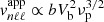 in the exponential case and
  in the Gaussian case. We see that a decrease in Vb of 30% leads to a decrease by a factor of two in
  , while an increase of b or νp by a factor of two results in an increase by a factor of between two or three. As the mode amplitudes are insignificantly low in the Gaussian case, such variations in the parameters, and even much larger variations, do not modify the large gap with the exponential case and the GOLF detection threshold; gravity modes thus remain undetectable in this case. In the exponential case, such variations in the parameters b and νp can in contrast affect the predictions about the detectability of the modes. Assuming an increase in νp by a factor of two, which results in an increase by a factor of about three in the amplitudes, the GOLF observation time required to detect a plume-induced dipolar gravity modes at νnℓm = 100 µHz is decreased by about one order of magnitude (i.e., to T ∼ 200 yr). Considering the largest plausible variations with a simultaneous increase in b by a factor of two, the observation time required to detect such a mode is reduced to T ∼ 50 yr. In this most favorable case considered here, the predicted amplitudes of the dipolar plume-induced gravity modes are plotted in Fig. 2 (blue dash-dotted line). This upper limit turns out to be close to the amplitudes of the turbulent-induced gravity modes predicted by Belkacem et al. (2009).
In conclusions, the time evolution of the plumes at the base of the convective zone represents the major source of uncertainties in our model. The error related to the uncertainties on the plumes parameters is insignificant compared to the effect of the assumption on the plume time evolution. In addition, while the plume-induced gravity modes remain undetectable in the Gaussian assumption whatever the values of the plume parameters, the uncertainties on these parameters can significantly modify the predictions of the detectability of few modes in the exponential assumption. In the most favorable plausible case, the GOLF observation time required to detect the plume-induced ℓ = 1 gravity modes around νnℓm ≈ 100 µHz is reduced to T ∼ 50 yr, with amplitudes close to those predicted considering turbulent pressure as the driving mechanism.
4.4. Can the amplitudes of gravity modes bring constraints on penetrative convection?
We see in Sect. 4.3 that our lack of knowledge on penetrative convection affects our predictions. In turn, we can wonder to what extent the measurement of the amplitudes of gravity modes in the Sun can provide us with constraints on penetrative convection and the properties at the base of the convective zone.
Our model shows either that the contribution from penetrative convection to the mode amplitude is undetectable for a Gaussian-like plume time evolution or that it behaves as a function of the frequency and the degree in a similar way to the contribution from turbulent convection for an exponential plume time profile. As both excitation mechanisms are subject to uncertainties (Belkacem et al. 2009), it can thus appears difficult at first sight to disentangle the two contributions and interpret the observed amplitudes in terms of structure without any independent information. Assuming that the plume time evolution is exponential, the measurement of the mode amplitude can nevertheless easily put upper limits on each excitation process, by ensuring that the predictions in each case remain lower than the observations. As the solar gravity modes have not been detected yet, we can similarly proceed by ensuring that the predictions remain lower than the current detection threshold. Imposing that  for νnℓm = 100 µHz and ℓ = 1 in the exponential case, we find, using Eqs. (15), (18), (19) and (25), that for 22-year GOLF observations
 (26)
(26)
where L⊙ is the solar luminosity.
Although the potential of the gravity mode amplitudes to probe penetrative convection is highlighted here, the present work suggests that the current theoretical uncertainties on the modeling of penetrative convection, and in particular on the plume time evolution, would limit their physical interpretation. The issue of disentangling the contributions of different sources to the excitation is especially brought to the fore. Theoretical efforts, by means of numerical simulations and semi-analytical models, and possible complementary observational constraints will be needed in the future to improve our modeling of this phenomenon and to elaborate relevant and robust seismic diagnoses to interpret the amplitude of gravity modes.
5. Conclusions
In this work our aim was to estimate the amplitude of the asymptotic solar gravity modes generated by penetrative convection in the frequency range between 10 µHz and 100 µHz. Following Pinçon et al. (2016), we considered the ram pressure of an ensemble of incoherent, uniformly distributed convective plumes penetrating into the top layers of the radiative zone as the driving mechanism. The forced oscillation equation was solved in the global quasi-adiabatic approximation using a two-timing method. As a result, we obtain an analytical expression of the mean mode energy, which is converted into apparent radial mode velocity through appropriate visibility factors. The standard plume modeling (i.e., plume radius, velocity, and lifetime) follows semi-analytical models, and their time evolution in the penetration region is assumed to be either Gaussian or exponential, by analogy with stochastic excitation by turbulent eddies. The apparent mode radial velocity is computed for a solar model in both cases and the result is compared to the 22-year GOLF detection threshold.
We find that the mean mode energy drastically depends on the assumption about the time evolution of the plumes inside the penetration region. On the one hand, in the limiting case of a Gaussian time evolution, asymptotic gravity modes turn out to be undetectable by means of radial velocity measurements such as those performed by the GOLF instrument. This is the consequence of a plume lifetime that is too long compared to the oscillation period. This result holds true despite a wide range of values considered for the parameters of the model. In the other limiting case of an exponential time evolution we find that penetrative convection can generate gravity modes in a much more efficient way than in the Gaussian case. In this case, the lower the angular degree or the higher the frequency, the larger the apparent mode radial velocity. Using standard values for the plume parameters, the apparent radial mode velocity appears to reach about 0.05 cm s−1 for ℓ = 1 and νnℓm ≈ 100 µHz. These predictions are one order of magnitude smaller than those predicted considering turbulent pressure as the driving mechanism, and remain well below the current 22-year GOLF detection threshold. Nevertheless, accounting for uncertainties in the plume parameters, we find in the most favorable plausible case that the predicted apparent mode radial velocity can be increased by a factor of six, that is, around 0.3 cm s−1 for ℓ = 1 and νnℓm ≈ 100 µHz. The observation time required to detect such a mode is reduced to about 50 yr with the GOLF instrument. These variations mainly result from an important sensitivity of the mode amplitude to the plume parameters, and, in contrast, from a limited sensitivity of the detection threshold to the observation time. Our findings thus indicate that, in the most favorable plausible case, penetrative convection can drive asymptotic gravity modes as efficiently as turbulent convection and with amplitudes close to the detection limit. We highlight that, if detected, the measurement of the gravity mode amplitudes is expected to bring constraints on penetrative convection, but that the current uncertainties on the modeling of penetrative convection, and in particular their temporal evolution, will certainly limit their physical interpretation.
The results of this work call for further studies, either observational or theoretical. First, our estimate of the excitation by penetrative plumes and the previous estimates of the excitation by turbulent pressure clearly suggest that we are likely to be very close to the detection in the asymptotic frequency range, and encourage us to carry on our efforts in observations and data analyses. While we mainly focused on the 22-year GOLF data, we note that a myriad of other data is available, for instance the observations by the GONG and BiSON ground-based telescope networks, and are an important source of information to be analyzed. Second, it will be interesting in the future to extend the theoretical predictions to a higher frequency range. A simple extrapolation of the available predictions toward slightly higher frequencies suggests that the amplitudes of the gravity modes in this domain are also likely to be close to the current detection limit. As already pointed out by Belkacem et al. (2011), predicting the amplitude of such low radial order gravity modes will require us to account consistently for the interplay between oscillations and convection, which is challenging since it will call for combining a proper non-local time-dependent treatment of convection with a fully non-adiabatic treatment of pulsations. Furthermore, new developments, based both on numerical simulations and semi-analytical models, are needed to improve our understanding of the behavior of downward convective plumes at the interface with the radiative region. Although it is still a challenge to accurately simulate stellar regimes, our hope is that the promising combination of such theoretical advancements with future measurements of the gravity mode amplitudes will bring constraints on the dynamics and the mixing at work at the base of the convective zone.
The Lagrangian variation of the mean molecular weight is usually neglected because the microscopic diffusion and nuclear timescales are supposed to be much longer than the oscillation timescale.
In this paper the local norm of a linear operator ℒ acting on a vector X(r) in the vicinity of a point r0 is defined as
![Mathematical equation: $$ \begin{aligned} \mathcal{N} _X(\boldsymbol{r}_0)=\max _{\boldsymbol{r}\in C_0} \left( \frac{\left|\mathcal{L} [X(\boldsymbol{r})]\right|}{ \left|X(\boldsymbol{r})\right| }\right), \end{aligned} $$](/articles/aa/full_html/2021/06/aa40003-20/aa40003-20-eq71.gif) (A.15)
(A.15)
where (|⋅|) is the modulus and C0 represents the volume of the sphere of center r0 with a radius equal to the local characteristic wavelength λ(r0) of the vector X, excluding the nodes where X(r) = 0.
The time Fourier transform of a function X(r, t) is defined as
![Mathematical equation: $ \mathcal{T}_{\mathrm{F}}[X]=\hat{X}(\boldsymbol{r},\omega)=\int_{-\infty}^{+\infty} X(\boldsymbol{r},t) \ e^{-i\omega t} {{\textrm{d}}}t . $](/articles/aa/full_html/2021/06/aa40003-20/aa40003-20-eq72.gif)
Acknowledgments
We thank the anonymous referee for his careful reading and relevant comments that greatly helped improving the manuscript. We sincerely acknowledge K. Belkacem and M.-A. Dupret for the very interesting discussions on the present subject and their sensible comments. During this work, C. P. was funded by a postdoctoral fellowship of Chargé de Recherche from F. R. S.-FNRS (Belgium). G. B. acknowledges fundings from the SNF AMBIZIONE grant No 185805 (Seismic inversions and modelling of transport processes in stars). C. P. warmly thanks M. Huet, V. Huet, A. Leguillon and C. Houdmond for their sincere friendship and their encouragements during the writing of this paper.
References
- Alvan, L., Brun, A. S., & Mathis, S. 2014, A&A, 565, A42 [NASA ADS] [CrossRef] [EDP Sciences] [Google Scholar]
- Andersen, B. N. 1994, Sol. Phys., 152, 241 [Google Scholar]
- Andersen, B. N. 1996, A&A, 312, 610 [NASA ADS] [Google Scholar]
- Appourchaux, T., Belkacem, K., Broomhall, A.-M., et al. 2010, A&ARv, 18, 197 [Google Scholar]
- Appourchaux, T., & Corbard, T. 2019, A&A, 624, A106 [NASA ADS] [CrossRef] [EDP Sciences] [Google Scholar]
- Appourchaux, T., & Pallé, P. L. 2013, in The History of the g-mode Quest, eds. K. Jain, S. C. Tripathy, F. Hill, J. W. Leibacher, & A. A. Pevtsov, ASP Conf. Ser., 478, 125 [Google Scholar]
- Appourchaux, T., Fröhlich, C., Andersen, B., et al. 2000, ApJ, 538, 401 [Google Scholar]
- Asplund, M., Grevesse, N., Sauval, A. J., & Scott, P. 2009, ARA&A, 47, 481 [NASA ADS] [CrossRef] [Google Scholar]
- Basu, S., & Antia, H. M. 2008, Phys. Rep., 457, 217 [Google Scholar]
- Belkacem, K. 2011, in Amplitudes of Solar Gravity Modes, eds. J. P. Rozelot, & C. Neiner, 832, 139 [Google Scholar]
- Belkacem, K., Samadi, R., Goupil, M. J., et al. 2009, A&A, 494, 191 [NASA ADS] [CrossRef] [EDP Sciences] [Google Scholar]
- Berthomieu, G., & Provost, J. 1990, A&A, 227, 563 [NASA ADS] [Google Scholar]
- Böning, V. G. A., Hu, H., & Gizon, L. 2019, A&A, 629, A26 [EDP Sciences] [Google Scholar]
- Bonventre, R., & Orebi Gann, G. D. 2018, Eur. Phys. J. C, 78, 435 [EDP Sciences] [Google Scholar]
- Brookes, J. R., Isaak, G. R., & van der Raay, H. B. 1976, Nature, 259, 92 [Google Scholar]
- Bruls, J. H. M. J., & Rutten, R. J. 1992, A&A, 265, 257 [NASA ADS] [Google Scholar]
- Brummell, N. H., Clune, T. L., & Toomre, J. 2002, ApJ, 570, 825 [Google Scholar]
- Buldgen, G. 2019, Bull. Soc. R. Sci. Liege, 88, 50 [Google Scholar]
- Buldgen, G., Eggenberger, P., Baturin, V. A., et al. 2020, A&A, 642, A36 [EDP Sciences] [Google Scholar]
- Chandrasekhar, S. 1964, ApJ, 139, 664 [Google Scholar]
- Christensen-Dalsgaard, J. 2008, Ap&SS, 316, 113 [Google Scholar]
- Christensen-Dalsgaard, J. 2021, Liv Rev: Sol. Phys., 18, 2 [Google Scholar]
- Christensen-Dalsgaard, J., Proffitt, C. R., & Thompson, M. J. 1993, ApJ, 403, L75 [NASA ADS] [CrossRef] [Google Scholar]
- Delache, P., & Scherrer, P. H. 1983, Nature, 306, 651 [Google Scholar]
- Dintrans, B., & Rieutord, M. 2001, MNRAS, 324, 635 [Google Scholar]
- Dintrans, B., Brandenburg, A., Nordlund, Å., & Stein, R. F. 2005, A&A, 438, 365 [NASA ADS] [CrossRef] [EDP Sciences] [Google Scholar]
- Dziembowski, W. 1977a, Acta Astron., 27, 95 [NASA ADS] [Google Scholar]
- Dziembowski, W. 1977b, Acta Astron., 27, 203 [NASA ADS] [Google Scholar]
- Dziembowski, W. A., Gough, D. O., Houdek, G., & Sienkiewicz, R. 2001, MNRAS, 328, 601 [Google Scholar]
- Edelmann, P. V. F., Ratnasingam, R. P., Pedersen, M. G., et al. 2019, ApJ, 876, 4 [Google Scholar]
- Eggenberger, P., Buldgen, G., & Salmon, S. J. A. J. 2019a, A&A, 626, L1 [NASA ADS] [CrossRef] [EDP Sciences] [Google Scholar]
- Eggenberger, P., Deheuvels, S., Miglio, A., et al. 2019b, A&A, 621, A66 [NASA ADS] [CrossRef] [EDP Sciences] [Google Scholar]
- Fossat, E., & Schmider, F. X. 2018, A&A, 612, L1 [NASA ADS] [CrossRef] [EDP Sciences] [Google Scholar]
- Fossat, E., Boumier, P., Corbard, T., et al. 2017, A&A, 604, A40 [NASA ADS] [CrossRef] [EDP Sciences] [Google Scholar]
- Gabriel, A. H., Grec, G., Charra, J., et al. 1995, Sol. Phys., 162, 61 [NASA ADS] [CrossRef] [Google Scholar]
- García, R. A., Turck-Chièze, S., Jiménez-Reyes, S. J., et al. 2007, Science, 316, 1591 [Google Scholar]
- Gehan, C., Mosser, B., Michel, E., Samadi, R., & Kallinger, T. 2018, A&A, 616, A24 [NASA ADS] [CrossRef] [EDP Sciences] [Google Scholar]
- Godart, M., Noels, A., Dupret, M.-A., & Lebreton, Y. 2009, MNRAS, 396, 1833 [Google Scholar]
- Gough, D. O. 1985, in Future Missions in Solar, Heliospheric & Space Plasma Physics, eds. E. Rolfe, & B. Battrick, ESA Spec. Pub., 235, 183 [Google Scholar]
- Kevorkian, J. 1961, PhD Thesis, California Institute of Technology, USA [Google Scholar]
- Kiraga, M., Stepien, K., & Jahn, K. 2005, Acta Astron., 55, 205 [NASA ADS] [Google Scholar]
- Kosovichev, A. G. 2011, in Advances in Global and Local Helioseismology: An Introductory Review, eds. J. P. Rozelot, & C. Neiner, 832, 3 [Google Scholar]
- Kumar, P., Quataert, E. J., & Bahcall, J. N. 1996, ApJ, 458, L83 [Google Scholar]
- Lecoanet, D., & Quataert, E. 2013, MNRAS, 430, 2363 [Google Scholar]
- Ledoux, P. 1951, ApJ, 114, 373 [Google Scholar]
- Lighthill, J. 1978, Waves in Fluids (Cambridge: Cambridge University Press) [Google Scholar]
- Lopes, I., & Turck-Chièze, S. 2014, ApJ, 792, L35 [Google Scholar]
- Marques, J. P., Goupil, M. J., Lebreton, Y., et al. 2013, A&A, 549, A74 [NASA ADS] [CrossRef] [EDP Sciences] [Google Scholar]
- Mussack, K., & Däppen, W. 2011, ApJ, 729, 96 [Google Scholar]
- Pieri, A. B., Falasca, F., von Hardenberg, J., & Provenzale, A. 2016, Phys. Lett. A, 380, 1363 [Google Scholar]
- Pinçon, C. 2017, Theses, PSL Research University, France [Google Scholar]
- Pinçon, C., Belkacem, K., & Goupil, M. J. 2016, A&A, 588, A122 [NASA ADS] [CrossRef] [EDP Sciences] [Google Scholar]
- Pinçon, C., Belkacem, K., Goupil, M. J., & Marques, J. P. 2017, A&A, 605, A31 [NASA ADS] [CrossRef] [EDP Sciences] [Google Scholar]
- Pratt, J., Baraffe, I., Goffrey, T., et al. 2017, A&A, 604, A125 [NASA ADS] [CrossRef] [EDP Sciences] [Google Scholar]
- Rempel, M. 2004, ApJ, 607, 1046 [Google Scholar]
- Rieutord, M., & Zahn, J.-P. 1995, A&A, 296, 127 [Google Scholar]
- Rogers, T. M., Glatzmaier, G. A., & Jones, C. A. 2006, ApJ, 653, 765 [Google Scholar]
- Rogers, T. M., Lin, D. N. C., McElwaine, J. N., & Lau, H. H. B. 2013, ApJ, 772, 21 [Google Scholar]
- Scherrer, P. H., & Gough, D. O. 2019, ApJ, 877, 42 [Google Scholar]
- Schunker, H., Schou, J., Gaulme, P., & Gizon, L. 2018, Sol. Phys., 293, 95 [Google Scholar]
- Severnyi, A. B., Kotov, V. A., & Tsap, T. T. 1976, Nature, 259, 87 [Google Scholar]
- Shibahashi, H. 1979, PASJ, 31, 87 [NASA ADS] [Google Scholar]
- Stein, R. F., & Nordlund, A. 1998, ApJ, 499, 914 [Google Scholar]
- Tassoul, M. 1980, ApJ, 43, 469 [Google Scholar]
- Thomson, D. J., Maclennan, C. G., & Lanzerotti, L. J. 1995, Nature, 376, 139 [NASA ADS] [CrossRef] [Google Scholar]
- Thompson, M. J., Christensen-Dalsgaard, J., Miesch, M. S., & Toomre, J. 2003, ARA&A, 41, 599 [NASA ADS] [CrossRef] [Google Scholar]
- Townsend, A. A. 1966, J. Fluid Mech., 24, 307 [Google Scholar]
- Turck-Chièze, S., García, R. A., Couvidat, S., et al. 2004, ApJ, 604, 455 [Google Scholar]
- Turner, J. S. 1986, J. Fluid Mech., 173, 431 [Google Scholar]
- Ulrich, R. K., Boumier, P., Robillot, J. M., et al. 2000, A&A, 364, 816 [Google Scholar]
- Unno, W., Osaki, Y., Ando, H., Saio, H., & Shibahashi, H. 1989, Nonradial Oscillations of Stars (Tokyo: University of Tokyo Press) [Google Scholar]
- von Hardenberg, J., Parodi, A., Passoni, G., Provenzale, A., & Spiegel, E. A. 2008, Phys. Lett. A, 372, 2223 [Google Scholar]
- Zahn, J.-P. 1991, A&A, 252, 179 [NASA ADS] [Google Scholar]
Appendix A: Energy spectrum of plume-induced gravity modes
In the following we derive the energy spectrum of asymptotic gravity modes generated by penetrative convection. The mathematical derivation largely uses and sometimes extends the analysis of stellar oscillations presented in Unno et al. (1989), and also uses the model of Pinçon et al. (2016).
A.1. Forced oscillation equations
Following the model of Pinçon et al. (2016), the linearized momentum, continuity, Poisson’s equations, and the equation of state1 read
 (A.1)
(A.1)
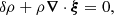 (A.2)
(A.2)
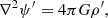 (A.3)
(A.3)
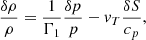 (A.4)
(A.4)
where p and g are respectively the equilibrium pressure and gravitational acceleration, ψ′ is the perturbation of the gravitational potential, Γ1 is the first adiabatic index, G is the gravitation constant, vT = −(∂lnρ/∂lnT)p, and all the other quantities are introduced in Sect. 2.1. In these four equations, X′ and δX denotes the Eulerian and Lagrangian perturbations of the quantity X, respectively. Using the usual solution of Poisson’s equation
 (A.5)
(A.5)
where V is the stellar volume beyond which the stellar density vanishes, as well as Eqs. (A.2) and (A.4), it is possible to rewrite Eq. (A.1) in the form of Eq. (1) in which
 (A.6)
(A.6)
with H = −(dr/dlnT) the temperature scale height and T the equilibrium temperature, and where ℒad is the adiabatic differential linear operator defined as (e.g., Chandrasekhar 1964; Unno et al. 1989, see Chap. 14.3 for details)
![Mathematical equation: $$ \begin{aligned}&\boldsymbol{\mathcal{L} }^\mathrm{ad}\left( \boldsymbol{\xi }\right)=\frac{\boldsymbol{\nabla } p}{\rho ^2} \boldsymbol{\nabla } \cdot \left(\rho \boldsymbol{\xi }\right) -\frac{1}{\rho } \boldsymbol{\nabla } \left( \boldsymbol{\xi }\cdot \boldsymbol{\nabla } p\right) -\frac{1}{\rho } \boldsymbol{\nabla } \left( \rho c^2\boldsymbol{\nabla }\cdot \boldsymbol{\xi } \right)\nonumber \\&\qquad \qquad + \boldsymbol{\nabla } \left( \int _{V} G \frac{\boldsymbol{\nabla }_{\boldsymbol{x}}\cdot \left[\rho (\boldsymbol{x}) \boldsymbol{\xi }(\boldsymbol{x}) \right] }{|\boldsymbol{r}-\boldsymbol{x}|} {\text{ d}}\boldsymbol{x}^3 \right) , \end{aligned} $$](/articles/aa/full_html/2021/06/aa40003-20/aa40003-20-eq79.gif) (A.7)
(A.7)
with c2 = Γ1p/ρ the squared sound speed. We note that H has been introduced in Eq. (A.6) for ℒnad to represent the same physical quantity as ℒad (i.e., a squared frequency). Equation (1) has to be completed by the energy equation that specifies the evolution of δS. Neglecting the contribution of the convective flux for asymptotic gravity modes (Belkacem et al. 2009) and the nuclear energy production rate in the considered layers, it reads
 (A.8)
(A.8)
where ℱR is the radiative flux.
A.2. Mode amplitude
A.2.1. Energy equation in the diffusion approximation
At this stage the oscillation equations are represented by Eqs. (1) and (A.8). Furthermore, we thus need to express the Lagrangian perturbation of the radiative flux. In the diffusion approximation the radiative flux is equal to
 (A.9)
(A.9)
where Krad is the radiative diffusivity, σSB is the Stefan-Boltzmann constant, and κ is the Rosseland mean opacity. Perturbing this equation and replacing δρ/ρ by −∇ ⋅ ξ, Eq. (A.8) can be rewritten
![Mathematical equation: $$ \begin{aligned}&\partial _t \left( \frac{\delta S}{c_p} \right) =-\frac{1}{\rho c_p T} \boldsymbol{\nabla }\cdot \left[-F_{\rm R}H\boldsymbol{\nabla }\left(\frac{\delta T}{T} \right) +\left(4\frac{\delta T}{T}+\boldsymbol{\nabla }\cdot \boldsymbol{\xi }-\frac{\delta \kappa }{\kappa } \right)\boldsymbol{F}_{\rm R}\right]\nonumber \\&\qquad \qquad +\frac{1}{\rho c_p T} \boldsymbol{\nabla }\cdot \left[\boldsymbol{\nabla } \left(\boldsymbol{F}_{\rm R}\cdot \boldsymbol{\xi }\right)-\boldsymbol{\xi }\left(\boldsymbol{\nabla }\cdot \boldsymbol{F}_{\rm R} \right)\right] , \end{aligned} $$](/articles/aa/full_html/2021/06/aa40003-20/aa40003-20-eq82.gif) (A.10)
(A.10)
where FR = FRer is the radial equilibrium radiative flux. We note that the right-hand side of Eq. (A.10) is equivalent to the right-hand side of Eq. (21.14) of Unno et al. (1989) with δεN = 0. Considering the equation of state T(S, ρ) and the opacity table κ(T, ρ) while using the continuity equation, it becomes
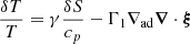 (A.11)
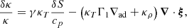 (A.12)
where γ = cp/cV, with cp and cV the specific heat capacities at constant pressure and volume, respectively; ∇ad is the adiabatic temperature gradient; κT = (∂lnκ/∂lnT)ρ; and κρ = (∂lnκ/∂lnρ)T. Using Eqs. (A.11) and (A.12) in Eq. (A.10), the evolution of the Lagrangian perturbation of entropy is ruled by
![Mathematical equation: $$ \begin{aligned} \partial _t \left( \frac{\delta S}{c_p} \right)=\frac{1}{t_{\rm R}} \left[ \mathcal{L} ^{\mathrm{nad}1}\left( \frac{\boldsymbol{\xi }}{H}\right)+\mathcal{L} ^{\mathrm{nad}2}\left( \frac{\delta S}{c_p}\right)\right] , \end{aligned} $$](/articles/aa/full_html/2021/06/aa40003-20/aa40003-20-eq85.gif) (A.13)
(A.13)
where we have introduced the local radiative thermal timescale
 (A.14)
and where ℒnad1 and ℒnad2 are two linear operators that involve derivatives with respect to the normalized variable r/H and whose expressions can be readily deduced from Eqs. (A.10)–(A.12).
A.2.2. Local scaling of the oscillation equations
Before going further, it is instructive to express locally the oscillation equations in a dimensionless form. In the following we focus on a mode with a characteristic angular frequency and a local wavelength denoted σ and λ(r, σ), respectively. The dynamical timescale is thus defined as tdyn ≡ σ−1. First, according to Eq. (4), the local norm of the ℒad operator2 is equal to σ2 for such a mode. Owing to the place of ℒnad in Eq. (1), it seems reasonable to assume that its norm also scales as σ2. This hypothesis is checked a posteriori in Sect. A.3.4. Equation (1) can thus be rewritten as
 (A.16)
where we have defined τ = t/tdyn and the differential operators  and
and  such that their norms remain on the order of unity. Second, regarding the energy equation, we first note that, owing to the incompressible character of the asymptotic low-frequency gravity modes (e.g., Dintrans & Rieutord 2001),
 (A.17)
where the big-𝒪 Bachmann-Landau notation is introduced. As ℒnad1 and ℒnad2 in Eq. (A.13) involve third-order and second-order derivatives at most with respect to r/H of ∇ ⋅ ξ and δS/cp, respectively, their norms thus at most scale as (H2/λ2) since λ ≲ H and Eq. (A.17) are met within the asymptotic limit. Equation (A.13) can hence be locally expressed as
![Mathematical equation: $$ \begin{aligned} \partial _\tau \left( \frac{\delta S}{c_p} \right)=\varepsilon _{\sigma } \left[ \tilde{\mathcal{L} }^{\mathrm{nad}1}\left( \frac{\boldsymbol{\xi }}{H}\right)+\tilde{\mathcal{L} }^{\mathrm{nad}2}\left( \frac{\delta S}{c_p}\right)\right] . \end{aligned} $$](/articles/aa/full_html/2021/06/aa40003-20/aa40003-20-eq91.gif) (A.18)
(A.18)
In this equation, we have defined
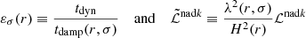 (A.19)
in such a way that the norms of  for k = 1, 2 also remain on the order of unity, and where we can identify the local damping timescale as
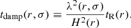 (A.20)
A.2.3. Globally quasi-adiabatic oscillations
At this point, we focus on a component (n, ℓ, m) with the amplitude anℓm(t) and the frequency ωnℓm, and fix σ = ωnℓm and εσ ≡ εnℓm. According to Eq. (A.18), δS locally scales as
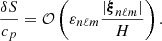 (A.21)
In a given frequency range around ωnℓm the damping timescale is expected to be much longer than the oscillation period almost everywhere in the star. As a result, εnℓm ≪ 1 and δS/cp ≪ |ξnℓm|/H. In the limit of εnℓm → 0, δS → 0 and the problem locally tends toward the adiabatic case. Nevertheless, there obviously exists a very thin near-surface layer where εnℓm ≫ 1 and the quasi-adiabatic approximation locally fails, so that the ordering in Eq. (A.21) is not met. Therefore, in order to reason from a global point of view, we define the global damping timescale as the inverse of the harmonic mean of the local damping timescale throughout the star weighted by the local mode energy, that is,
 (A.22)
where Tdamp has to be related to the local wavelength of ξnℓm through Eqs. (A.20) and (A.22), and where ℳnℓm is the mode mass defined in Eq. (6). In the following we thus assume that the oscillations are globally quasi-adiabatic, that is,
 (A.23)
For convenience, we also define the quantity
 (A.24)
The global quasi-adiabatic approximation expressed by Eq. (A.23) will greatly ease the derivation of the mode amplitude, as we show here.
Taking the derivative of Eq. (A.16) with respect to τ, injecting Eqs. (3) and (A.18) into the obtained expression, and computing the inner product with  , we obtain a differential equation ruling the mode amplitude anℓm(τ). We point out that, owing to the spherical symmetry of the star, the inner product with
  selects the angular degree ℓ and the azimuthal number m in the expansion of the perturbations onto the orthonormal basis of the spherical harmonics (see, e.g., the definitions of the differential operators). Therefore, the subscript ℓm is often dropped to simplify the notation in what follows. The amplitude equation finally reads, at first order in δn,
 (A.25)
where
![Mathematical equation: $$ \begin{aligned}&\tilde{\eta }_{n n^\prime }=-\frac{1}{2 \chi _{n\ell m}}\int _{V}\rho \boldsymbol{\xi }_{n\ell m}^\star \cdot \tilde{\boldsymbol{\mathcal{L} }}^\mathrm{nad}\left[H\varepsilon _{n^\prime \ell m}\tilde{\boldsymbol{\mathcal{L} }}^\mathrm{nad1}\left(\frac{\boldsymbol{\xi }_{n^\prime \ell m}}{H}\right)\right] {\text{ d}}V,\end{aligned} $$](/articles/aa/full_html/2021/06/aa40003-20/aa40003-20-eq102.gif) (A.26)
(A.26)
 (A.27)
The second-order term in Eq. (A.25) is related to the Lagrangian perturbation of entropy and results from the scaling in Eq. (A.21) and the global quasi-adiabatic hypothesis in Eq. (A.23). In addition, the product  stands for the damping rate (in terms of the τ variable). In contrast, the sum in the brackets on the left-hand side of Eq. (A.25) encapsulates coupling terms between the components n and n′ ≠ n. Such coupling terms result, by construction, from the expansion onto the eigenfunctions of the ℒad operator as they are not natural solutions of the non-adiabatic problem. When writing Eq. (A.25), we have implicitly assumed
  . As shown in Eq. (A.26), the integral in the numerator is at most on the order of χnℓm since the norms of the operators are on the order of unity. Moreover, this integral corresponds to the inner product between an oscillating radial function, with n radial nodes and a characteristic wavelength λn, and another oscillating radial function, with about n′ radial nodes and a characteristic wavelength λn′. For n′ ∼ n we therefore have
  , whereas for n′ ≫ n or n′≪n both oscillating functions are incoherent with each other and the inner product vanishes, that is,
  . This justifies
  .
.
A.2.4. Two-timing analysis
As shown by Eq. (A.25), the evolution of the mode amplitude is ruled by a fast dynamical timescale, T0 = τ = t/tdyn, and a slow damping timescale, T1 = δnτ = t/Tdamp. Using a two-timing perturbation method therefore seems judicious to solve analytically this equation (e.g., Kevorkian 1961). This method can provide us with a uniformly valid solution up to a timescale on the order of 𝒪(1/δn) in terms of the independent variable τ, or equivalently 𝒪(Tdamp) in terms of the dependent variable t.
Homogeneous equation. Taking advantage of the linearity of the problem, we search in a first step for a general solution of the homogeneous amplitude equation. For all n, we start from the two-timing perturbation ansatz, that is,
 (A.28)
keeping in mind that τ, T0, and T1 also depend on n through the scaling by 1/ωnℓm. Injecting Eq. (A.28) into Eq. (A.25) and using ∂τ = ∂T0 + δn∂T1 via the chain rule, the homogeneous equation reads at leading order in δn
 (A.29)
and at first order in δn
 (A.30)
The general solution of Eq. (A.29) then reads
 (A.31)
where αn(T1) and βn(T1) are two functions to be determined with the first-order equation. Using Eq. (A.31) in Eq. (A.30), it is straightforward to show (e.g., via the method of variation of parameters) that, if non-null, the terms in brackets will induce terms proportional to τe±iτ in the expression of  , up to a factor on the order of αn and βn. This will make
  on the order of
  up to a timescale on the order of 𝒪(1/δn) and, therefore, would break the perturbation ansatz in Eq. (A.28). Therefore, to obtain a uniformly valid expression up to such timescales, the terms in brackets have to vanish. This condition leads to
 (A.32)
with An and Bn two arbitrary constants. As a consequence, the amplitude  is ruled only by the coupling term on the right-hand side of Eq. (A.30), which depends on the leading-order amplitudes
  with n′ ≠ n. For n′ ≠ n, it is obvious that the amplitudes follow the same zeroth-order and first-order equations as in Eqs. (A.29) and (A.30); however, because of the considered scaling, Tk for k = 0 or 1 in these equations are replaced by
 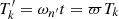 with ϖ = (ωn′/ωn). As a result, we get
 (A.33)
where An′ and Bn′ are two arbitrary constants. According to Eqs. (A.30)–(A.32) we thus find that  is ruled at leading order by
 (A.34)
Using again the method of variation of parameters, we can show that the amplitude  is equal to a series of terms as a function of n′ that are
  ). At this point, we assume that the magnitude of
  slowly varies with n′, so that it is
  for n′∼n; this will be checked a posteriori (see the resulting velocity amplitudes in Fig. 2). Provided
  for n ∼ n′ and
  otherwise, as justified in Appendix A.2.3, the main contribution to
  results from the terms of the series associated with n′ ∼ n; as a result,
  with Δωn = |ωn − ωn − 1|. Within the asymptotic limit, ωn/Δωn ∼ n ≫ 1 and thus
  in order of magnitude. This highlights afterward that, instead of δn, it is more appropriate to scale the non-adiabatic perturbation of the mode amplitude by
 (A.35)
in such a way that the perturbation ansatz becomes
 (A.36)
and the new first-order perturbation  . As a result, the relative error when considering
  up to a timescale on the order of Tdamp is on the order of
  . We check a posteriori at the end of Sect. 3.1 that
  in the considered asymptotic frequency range. Therefore, all the previous perturbation developments, fortunately, hold true and the coupling terms do not stand for secular terms. These terms thus have no effect on the two-timing solution provided by
  , and are just responsible for the relative error on the order of
  .
.
In summary, provided that the mode amplitude slowly varies with the radial order, the solution of the homogeneous equation as a function of the variable t, which is uniformly valid up to a timescale on the order of 𝒪(Tdamp), takes the form, according to Eqs. (A.31) and (A.32), of the adiabatic solution modulated by an exponential damping term, that is,
 (A.37)
where the relative error is on the order of  and the damping rate is equal to
 (A.38)
with δn and  defined in Appendix A.2.3.
Physically speaking, we note that the parameter  measures the coupling induced by the non-adiabatic effects between adjacent harmonics in the decomposition onto the eigenfunctions of the ℒad operator. To show this, it is possible to express this parameter in more sensible ways. On the one hand, the eigenfrequencies of the adiabatic asymptotic gravity modes follow at leading order (e.g., Shibahashi 1979; Tassoul 1980)
 (A.39)
where ΔΠℓ is the so-called period-spacing, rb is the radius of the base of the convective zone, and N is the Brunt-Väisälä frequency defined as
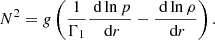 (A.40)
Therefore, for n ≫ 1 in the asymptotic regime, we have
 (A.41)
where kr is the local radial wavenumber. As the radial group velocity of gravity waves is about equal to ωn/kr (e.g., Unno et al. 1989), Eq. (A.41) shows that Δωn ∼ 1/Δtcore, where Δtcore is the time spent by a wave energy ray of frequency ωn to cross the radiative core. We thus obtain  . On the other hand, using ηn ∼ 1/Tdamp according to our scaling, we have
  . The hypothesis Eq. (12) is thus equivalent to assuming that the width of each oscillation peak around an adiabatic eigenfrequency is much smaller than the frequency spacing between two consecutive radial orders n and n + 1 in the power oscillation spectrum.
Forced amplitude. In a second step, we search for the solution of the forced amplitude equation that is uniformly valid up to timescales on the order of Tdamp and satisfies the initial value condition anℓm(−∞) = 0. Using the method of variation of parameters, it is straightforward to show that this solution is
 (A.42)
where An(t) is a function of time provided by Eq. (11) and Bn(t) = An(t)⋆. As a check, Eq. (A.42) leads to
 (A.43)
 (A.44)
Injecting Eqs. (A.43) and (A.44) in Eq. (A.25), we see that the secular term represented by 2ηnnan cancel out and that the relative residual is on the order of  at most, as shown in the previous paragraph.
A.3. Mean mode energy within the asymptotic limit
Within the asymptotic limit, it is possible to use, to good approximation, the leading-order WKB analytical expressions of the eigenfunctions in order to express the mean mode energy in a simple but sensible way.
A.3.1. General expression for the mean mode energy
Owing to the equipartition of the specific kinetic and potential energies in the case of gravity waves (e.g., Lighthill 1978), we define the mean total oscillation energy as
 (A.45)
where (⟨ ⋅ ⟩) is the (ensemble or time) mean operator and V represents the stellar volume.
To express Eq. (A.45) in a simple way, the same reasoning as done in Sects. 2.2.1 and 2.2.2 of Pinçon et al. (2016) can be used. While Pinçon et al. (2016) considered progressive wave packets propagating toward the center of the star and never returning back upward, it is in contrast necessary in the present case to consider the modal structure of the oscillations. The only difference is that, instead of considering that the lifetime of the wave packet at a certain point of the radiative zone is on the order of τp, as in Pinçon et al. (2016), we have to consider in the present case that the lifetime of the mode oscillation is on the order of Tdamp.
The reasoning is as follows. Owing to the linearity of the wave equations, the displacement field at any time can be represented as the superposition of all the waves induced by each individual plume. Each of these waves has a finite lifetime, which is on the order of the damping timescale Tdamp. Over the time interval [ − T/2, T/2], it thus appears obvious that the set of waves constituting ξ is generated by a finite number of plumes, denoted 𝒩T. In the limit of T ⋙ Tdamp, as the plume emerging rate is constant and equal to 𝒩/τp, with τp the characteristic plume lifetime, the number of penetrating plumes that contributes to ξ in the time interval [ − T/2, T/2] is equal at leading order to 𝒩T ∼ 𝒩νpT, with νp = 1/τp. Because of the incoherence of the convective plumes between each other, the wave velocity fields generated by different plumes negatively interfere. Assuming in addition that the excitation is a stationary process and that the plumes are all identical and uniformly distributed over the sphere, the time and volume integrals in Eq. (A.45) can be written as the mode energy associated with the displacement field ξ0(r, t; θ0, φ0) that is generated by one single plume penetrating at t0 = 0 in the solid angle dΩ0 = sin θ0dθ0dφ0 and with the velocity 𝒱p, 0, multiplied by the number of penetrating plumes over [ − T/2, T/2] (i.e., 𝒩T ∼ 𝒩νpT), and finally averaged over the plume angular position (θ0, φ0). Using the Parseval-Plancherel theorem in the time Fourier space, the mean mode energy can thus be expressed as
 (A.46)
where the symbol ( ) and ω respectively denotes the time Fourier transform and the temporal angular frequency3. Equation (A.46) can actually be retrieved through Eqs. (5) and (12) of Pinçon et al. (2016), but integrated over the volume of the star in the present case.
Furthermore, the mode displacement field ξ0 is expanded onto the eigenfunctions of the ℒad operator, similarly to Eq. (3), except that the instantaneous amplitude is induced only by the plume of velocity 𝒱p, 0, and thus depends on (θ0, φ0); it is denoted anℓm(t; θ0, φ0). Injecting such an expansion in Eq. (A.46) and using the orthogonality property of the adiabatic eigenfunctions, the mean total mode energy can be decomposed as
 (A.47)
where ⟨Enℓm⟩ is the mean oscillation energy of the harmonic (n, ℓ, m),
 (A.48)
with 𝒱nℓm the root mean square mode amplitude that reads
 (A.49)
To analytically express Eq. (A.49), it is thus sufficient to compute the amplitude from Eqs. (10) and (11) considering the model of plume velocity in Sect. 2.3.
A.3.2. Asymptotic form with our plume model
According to Sect. 2.3, we assume that the mode driving takes place in the nearly adiabatically stratified penetration region of length Lp where the plumes are braked by buoyancy. Based on the asymptotic analysis of gravity modes by Shibahashi (1979), the WKB expressions of the radial eigenfunctions of frequency ωnℓm, angular degree ℓ, and azimuthal number m in the penetration region are provided by Eq. (B.24) of Pinçon et al. (2016), which corresponds to an evanescent wave up to a constant Ac. In contrast, in the radiative zone, it is provided by the sum of Eqs. (B.25) and (B.26), which corresponds to the sum of a progressive and a regressive wave up to a complex constant Ar. The constants Ar and Ac have to be chosen in such a way to ensure the continuity of the radial and horizontal displacements at rb. This is met if |Ar/Ac|≈(Nt/ωnℓm)1/2 and |arg(Ar)| ≈ ωnℓ/Nt ≪ 1, in agreement with the more general computations of Lecoanet & Quataert (2013) or Pinçon et al. (2016).
First, using the WKB expressions of the eigenfunctions described above, Eqs. (10), (11), (A.27) and (13), the mean square mode velocity in Eq. (A.49) can be rewritten, after some algebraic manipulations and the computation of the Fourier transform of the mode amplitude, as
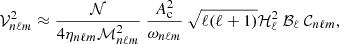 (A.50)
where ℋℓ and ℬℓ represent the radial and horizontal correlations between the plumes and the modes, whose expressions are provided by Eqs. (32)–(34) of Pinçon et al. (2016). The term 𝒞nℓm represents the temporal correlation that reads
 (A.51)
where we recall that f(t) is the plume time evolution profile. We note that the constant Ac at the numerator of Eq. (A.50) results from the inner product between the plume ram pressure and the eigenmode in the penetration region where the driving is assumed to be maximum (i.e., the volume integral in Eq. (A.27) is reduced to this region). Second, using again the asymptotic expression of the adiabatic eigenfunctions, and considering only the contribution from the radiative core where most of the mode energy is contained, the mode mass is equal at leading order to
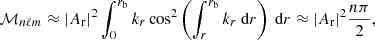 (A.52)
where we have used the quantization condition 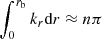 (see, e.g., Godart et al. 2009, for a similar computation). Finally, using Eqs. (A.50) and (A.52), the mean mode energy in Eq. (A.48) becomes
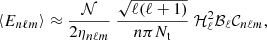 (A.53)
where we have used the continuity condition |Ac/Ar|2 = ωnℓm/Nt. Before going further, it is also instructive to express in a simple way the global damping timescale in Eq. (A.22) using the asymptotic form of the eigenfunctions. As explained in Sect. 2.2.2, we assume that the contribution from the upper layers to the integral in Eq. (A.22) is negligible compared to the contribution from the radiative cavity, as suggested by the numerical computations of Belkacem et al. (2009). Similarly to Eq. (A.52), in the asymptotic regime, ρ|ξnℓm|2 locally scales as |Ar|2/λnℓm, so that the global damping timescale can be reduced to the expression
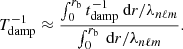 (A.54)
A.3.3. Temporal correlation 𝒞nℓm
The temporal correlation between the oscillation modes and the plumes in Eq. (A.51) depends on the time evolution of the plume in the driving zone. Using both the convolution and Cauchy’s residue theorems, we find in the exponential limiting case for f = fE
![Mathematical equation: $$ \begin{aligned} \mathcal{C} _{n\ell m}^\mathrm{E}=\frac{8\nu _{\rm p}^2 \ \omega _{n\ell m}\ (2\nu _{\rm p}+\eta _{n\ell m})}{\left[(2\nu _{\rm p}+\eta _{n\ell m})^2+\omega _{n\ell m}^2\right]^2} , \end{aligned} $$](/articles/aa/full_html/2021/06/aa40003-20/aa40003-20-eq166.gif) (A.55)
(A.55)
and in the Gaussian limiting case for f = fG
![Mathematical equation: $$ \begin{aligned} \mathcal{C} _{n\ell m}^\mathrm{G}=\pi \mathcal{I} _{m}\left\{ \ \zeta e^{+\zeta ^2}\left[ \mathrm{erf}(\zeta )-1\right]\ \right\} , \end{aligned} $$](/articles/aa/full_html/2021/06/aa40003-20/aa40003-20-eq167.gif) (A.56)
(A.56)
where ζ = (ηnℓm − iωnℓm)/2νp, ℐm() denotes the imaginary part, and erf() is the error function. When ηnℓm ≪ νp ≪ ωnℓm, we have to a good approximation
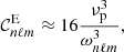 (A.57)
which results from the contribution from the resonant frequencies such as ω ∼ ωnℓm to the integral in Eq. (A.51), and
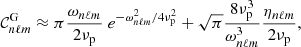 (A.58)
where the first term results from the contribution from the high frequencies such as ω ∼ ωnℓm to the integral in Eq. (A.51), while the second term results from the contribution from the low frequencies such as ω ≲ νp.
A.3.4. Damping rate
The expression of the damping rate ηnℓm is provided by Eq. (A.38). This expression is actually equivalent to the expression of the damping rate found by Godart et al. (2009) within the quasi-adiabatic and asymptotic limits. Using our notation, Eqs. (14) and (15) of Godart et al. (2009) can be rewritten in the form (see also Sect. 5.4.2 of Pinçon 2017)
![Mathematical equation: $$ \begin{aligned} \eta _{n\ell m}\approx \frac{[\ell (\ell +1)]^{3/2}}{2\omega _{n\ell m}^3} \frac{1}{n\pi } \int _0^{r_{\rm b}} \frac{H^2}{t_{\rm R}} N_T^2N \frac{{\text{ d}}r}{r^3} , \end{aligned} $$](/articles/aa/full_html/2021/06/aa40003-20/aa40003-20-eq170.gif) (A.59)
(A.59)
where H is the temperature scale height and NT is the part of the Brunt-Väisälä frequency related to the temperature gradient alone. According to Eqs. (A.39) and (A.41), Eq. (A.59) can be formulated as
 (A.60)
where we used  to write the inequality. Equation (A.60) shows that
  . Moreover, the local damping timescale was defined as tdamp ∼ (λ/H)2tR ∼ (krH)−2tR. Therefore, according to Eq. (A.54), ηnℓm turns out to be 𝒪(1/Tdamp). In addition, the comparison with the expression given by Eqs. (A.22), (A.26) and (A.38) confirms a posteriori the scaling of the norm of the ℒnad operator as
  and that of the ℒnad1 operators as H2/λ2, as assumed in Appendix A.2.2.
A.3.5. Simplified analytical expression
For small angular degrees, that is ℓ ≲ rb/b ∼ 50 for the Sun, which is sufficient for the present study, a very good analytical expression of ℬℓ is provided by Eq. (37) of Pinçon et al. (2016). Moreover, within the large Péclet number regime, the length of the penetration zone is expected to be much smaller than the characteristic decay length of the mode toward the surface. We recall that the mode is evanescent in this region and that its decay length is equal to  (e.g., Shibahashi 1979). As a consequence, the eigenfunctions slowly vary in the penetration region and the radial gradient of the plume ram pressure contained in ℋℓ can be seen as a Dirac function, so that we have in a good approximation
  . Pinçon et al. (2016) numerically demonstrated the validity of this simplification. Using both simplifications for ℬℓ and ℋℓ, Eq. (A.53) can be analytically expressed by Eq. (15).
Appendix B: Non-adiabatic mode displacement basis
According to Chandrasekhar (1964) or Unno et al. (1989), the eigenfunctions of the ℒad operator in Eq. (1) form, at each time, a complete basis of the displacement field over the stellar volume V (i.e., beyond which the stellar density vanishes, the so-called zero-boundary conditions) when the oscillations are adiabatic. In this section we show that this holds true in the non-adiabatic case.
To show this, limiting ourselves to non-rotating stars, it is actually sufficient to demonstrate the hermicity of the ℒad operator. To do so, we adapt the demonstration done in the adiabatic case by Unno et al. (1989, see Chaps. 14.2 and 14.3) to the non-adiabatic case. We consider two trial displacement fields, ξ and  , that are solutions of the non-adiabatic oscillation equations and that are expanded onto the spherical harmonics basis. First, computing the dot product of Eq. (1) with
  , where the superscript star (⋆) denotes the complex conjugate, using the continuity equation in Eq. (A.2), and integrating over the stellar volume, we obtain
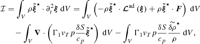 (B.1)
(B.1)
where F represents a given forcing term. Second, computing the dot product of Eq. (A.1) with  , and then proceeding as in Eq. (14.18) of Unno et al. (1989), i.e., expressing the left-hand side of the obtained expression in a flux-conservative form, using Eqs. (A.2) and (A.3), the hydrostatic equilibrium equation, as well as the equation of state in Eq. (A.4) rewritten as
 (B.2)
(B.2)
with N2 the square Brunt-Väisälä frequency provided in Eq. (A.40) and ξr the radial displacement, we obtain after some algebraic manipulations
 (B.3)
(B.3)
Owing to the zero-boundary conditions, the second integrals in Eqs. (B.1) and (B.3) vanish in virtue of the Green-Ostrogradsky theorem. Therefore, equating Eq. (B.1) with Eq. (B.3) and replacing  by Eq. (A.4), we find
![Mathematical equation: $$ \begin{aligned}&\int _{V} \rho \tilde{\boldsymbol{\xi }}^\star \cdot \boldsymbol{\mathcal{L} }^\mathrm{ad}\left(\boldsymbol{\xi } \right) {\text{ d}}V=\int _{V} \left( \frac{\tilde{p}^{\prime \star } p^\prime }{\rho c^2}+N^2\rho \tilde{\xi }_r^\star \xi _r-\frac{\boldsymbol{\nabla }\tilde{\psi }^{\prime \star }\cdot \boldsymbol{\nabla }\psi ^\prime }{4\pi G}\right){\text{ d}}V\nonumber \\&\qquad \quad -\sum _{\ell ,m}\frac{(\ell +1)}{4\pi G} \left[r\psi ^\prime _{\ell m}(r)\tilde{\psi }^{\prime \star }_{\ell m}(r)\right]_{r=R_V} \nonumber \\&\qquad \quad +\int _{V}\left(\Gamma _1{v}_T^2 p \frac{\widetilde{\delta S}^\star \delta S}{c_p^2}-{v}_T\left[p^\prime \frac{\widetilde{\delta S}^\star }{c_p}+\frac{\delta S}{c_p} \tilde{p}^{\prime \star }\right]\right){\text{ d}}V, \end{aligned} $$](/articles/aa/full_html/2021/06/aa40003-20/aa40003-20-eq184.gif) (B.4)
(B.4)
where ψℓm are the radial functions of the perturbation of the gravitational potential according to the expansion on the orthonormal spherical harmonics, and RV is the radius of the sphere of volume V. The first integral and the sum on the right-hand side of Eq. (B.4) correspond to the expression found by Unno et al. (1989) within the adiabatic hypothesis, the last term of which results from the zero-boundary conditions at r = RV, i.e., (dψℓm/dr) = − (ℓ+1)ψℓm/r according to Poisson’s equation with a null density. In contrast, the last integral on the right-hand side of Eq. (B.4) results from the non-adiabatic effects. Despite this difference, Eq. (B.4) remains symmetric with respect to  and ξ:
 (B.5)
(B.5)
Therefore, ℒad is Hermitian in the non-adiabatic case as well. According to the spectral theorem, the set of the eigenfunctions of ℒad also forms a basis of the displacement field over V in the non-adiabatic case. From Eq. (B.5) and the eigenvalue relation in Eq. (4), it is straightforward to demonstrate that these eigenfunctions are orthogonal.
Appendix C: Mean mode radial velocity
In this section we briefly summarize the computation of the mean apparent surface velocity following Appendix C in Belkacem et al. (2009).
First, we recall that in the slow rotation limit, which is valid for the considered frequency range in the Sun, the eigenfrequencies are slightly shifted as a function of ℓ and m around the value predicted in the non-rotating case (e.g., Ledoux 1951). The oscillation power spectrum of the solar gravity modes is thus composed of a forest of peaks, each of them associated with a tuple (n, ℓ, m). It is thus necessary to compute the mean apparent radial velocity for all these components. However, for the sake of simplicity, the computation is made to a first approximation by neglecting the effect of rotation on the spatial shape of the mode. Therefore, we assume the total mode displacement field ξ can still be expanded onto the eigenfunctions computed in the non-rotating case, that is,
 (C.1)
(C.1)
where  is an instantaneous amplitude, ξnℓm is normalized by the value of the radial displacement at the photosphere, and (r, θ, φ) is the spherical coordinate system in the observer’s frame such that the polar axis (i.e., θ = 0) corresponds to the direction of the stellar rotation axis and the origin (i.e., r = 0) corresponds to the stellar center. Under this approximation, the velocity component associated with the tuple (n, ℓ, m) is thus merely equal to
 (C.2)
(C.2)
Second, we define a spherical coordinate system (r, Θ, Φ) in the observer’s frame whose origin (i.e., r = 0) corresponds to the star center and the polar axis (i.e., Θ = 0) is directed toward the observer. Given the large distance from the observer, the direction of the line of sight can be considered equal to the unit vector n parallel to the polar axis. Moreover, owing to the small amplitudes of the oscillations near the stellar surface, the shell in which the considered absorption line forms remains undeformed at first order. Within this framework, each infinitesimal surface element d2Sabs of the absorption shell emits a number proportional to d2Nλ = h(µ) µ d2Sabs of photons at wavelength λ and per unit of time toward the observer, where µ = cos Θ, h(µ) is the limb-darkening function,  , and rabs is the radius of the considered shell. The mean radial velocity is therefore defined as the average of the radial velocity over the disk weighted by the number of photons received by the observer from each point of its surface (e.g. Dziembowski 1977a):
![Mathematical equation: $$ \begin{aligned} {v}_{n\ell m}^\mathrm{rad}=\dfrac{\int _0^1\int _0^{2\pi } \left[\boldsymbol{v}_{n\ell m}(r_{\rm abs},\Theta ,\Phi ,t)\cdot \boldsymbol{n}\right]h(\mu )\mu r_{\rm abs}^2{\text{ d}}\mu {\text{ d}}\Phi }{\int _0^1 \int _0^{2\pi }h(\mu )\mu r_{\rm abs}^2{\text{ d}}\mu {\text{ d}}\Phi } . \end{aligned} $$](/articles/aa/full_html/2021/06/aa40003-20/aa40003-20-eq191.gif) (C.3)
(C.3)
To go a step further, the mean apparent velocity is defined as the statistical or, equivalently for an ergodic process, time average quantity:
 (C.4)
(C.4)
Using Eqs. (C.2) and (C.3) and following all the derivation steps in Appendix C of Belkacem et al. (2009), it is straightforward to show that Eq. (C.4) is equal to
 (C.5)
(C.5)
with
 (C.6)
(C.6)
 (C.7)
(C.7)
where Θ0 is the angle between the rotation axis and the line of sight,  is the associated Legendre polynomial, and
  , uℓ, and vℓ are defined by
 (C.8)
(C.8)
 (C.9)
(C.9)
![Mathematical equation: $$ \begin{aligned}&{v}_\ell = \ell \int _{0}^1 \mu \tilde{h}(\mu )\left[P_{\ell -1}(\mu ) -\mu P_\ell (\mu )\right]{\text{ d}}\mu , \end{aligned} $$](/articles/aa/full_html/2021/06/aa40003-20/aa40003-20-eq200.gif) (C.10)
(C.10)
in which the  function must be replaced by the properly normalized limb darkening function, that is,
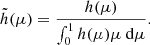 (C.11)
Finally, according to Eq. (C.1) and the orthogonality of the eigenfunctions, it is straightforward to show that the mean square amplitude is provided by
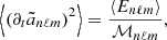 (C.12)
where ⟨Enℓm⟩ is the mean mode energy for the tuple (n, ℓ, m) given in Eq. (A.48) and ℳnℓm is the mode mass in Eq. (6). Therefore, the apparent velocity in Eq. (C.5) can be rewritten as in Eqs. (19) and (20).
Appendix D: GOLF detection threshold
According to Appourchaux et al. (2000), the threshold signal-to-noise ratio above which a peak over a frequency interval Δf in the power spectral density (PSD) can be considered a statistically relevant signal is equal to
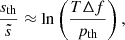 (D.1)
(D.1)
where  is the mean noise level over Δf and pth is the false alarm probability that the measurement is due to pure noise. We note that the frequency interval Δf in Eq. (D.1) must be small enough for the PSD to remain about constant over this range, but large enough for the number of frequency bins inside to be high enough. The mean noise level between 10 µHz and 100 µHz can be estimated in a simple way, for example, through the analysis of the 10-year GOLF data of García et al. (2007, see Fig. S1.):
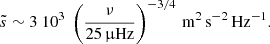 (D.2)
(D.2)
The value of the PSD at the level of detection (i.e., sth) can then be converted into a threshold value vth for the root mean square velocity by integrating the PSD over one frequency bin of width 1/T and computing the square root of the result, leading to Eq. (25). We note that the expression of the mean noise level provided in Eq. (D.2) is sufficient for our purpose since the threshold velocity depends on  only to the power 1/2, and thus is little impacted by the error made with our simple estimate of the magnitude and the frequency exponent in this expression.
All Tables
Absolute values of the visibility factors of the GOLF instrument as a function of the angular degree ℓ.
All Figures
|
Fig. 1. Radiative damping rate as a function of the oscillation frequency νnℓm and the angular degree ℓ. Each circle corresponds to a given eigenmode. |
| In the text | |
|
Fig. 2. Apparent surface radial velocity of solar gravity modes as a function of the oscillation frequency νnℓm and the angular degree ℓ, for azimuthal numbers m = ℓ and for standard plume parameters. The results obtained with a Gaussian and an exponential plume time evolution (see Sect. 2.3) are represented by the diamonds and the plus signs, respectively, for each considered eigenmode. The thick dashed gray line corresponds to the 22-year GOLF detection threshold (see Sect. 3.3). The blue dash-dotted line represents the upper limit for the amplitude of the dipolar modes when accounting for the largest plausible variations in the plume parameters (i.e., with a factor of two increase in the inverse plume lifetime and radius; see Sect. 4.3). |
| In the text | |
Current usage metrics show cumulative count of Article Views (full-text article views including HTML views, PDF and ePub downloads, according to the available data) and Abstracts Views on Vision4Press platform.
Data correspond to usage on the plateform after 2015. The current usage metrics is available 48-96 hours after online publication and is updated daily on week days.
Initial download of the metrics may take a while.