| Issue |
A&A
Volume 650, June 2021
Parker Solar Probe: Ushering a new frontier in space exploration
|
|
|---|---|---|
| Article Number | A31 | |
| Number of page(s) | 14 | |
| Section | The Sun and the Heliosphere | |
| DOI | https://doi.org/10.1051/0004-6361/202039490 | |
| Published online | 02 June 2021 | |
Coronal mass ejections observed by heliospheric imagers at 0.2 and 1 au
The events on April 1 and 2, 2019
1
George Mason University, 4400 University Drive,
Faixfax,
VA
22030,
USA
e-mail: cbraga@gmu.edu
2
The Johns Hopkins University Applied Physics Laboratory,
Laurel,
MD
20723,
USA
Received:
21
September
2020
Accepted:
7
November
2020
Context. We study two coronal mass ejections (CMEs) observed between April 1 to 2, 2019 by both the inner Wide-Field Imager for Parker Solar Probe (WISPR-I) onboard the Parker Solar Probe (PSP) spacecraft (located between about 46 and 38 solar radii during this period) and the inner heliospheric imager (HI-1) onboard the Solar Terrestrial Relations Observatory Ahead (STEREO-A) spacecraft, orbiting the Sun at about 0.96 au. This is the first study of CME observations from two viewpoints in similar directions but at considerably different solar distances.
Aims. Our objective is to derive CME kinematics from WISPR-I observations and to compare them with results from HI-1. This allows us to understand how the PSP observations affect the CME kinematics, especially due to its proximity to the Sun.
Methods. We estimated the CME positions, speeds, accelerations, propagation directions, and longitudinal deflections using imaging observations from two spacecrafts and a set of analytical expressions that consider the CME as a point structure and take the rapid change in spacecraft position into account. We derived the kinematics using each viewpoint independently and both viewpoints as a constraint.
Results. We found that both CMEs are slow (<400 km s−1), propagating eastward of the Sun-Earth line (westward of PSP and STEREO-A). The second CME seems to accelerate between ~0.1 and ~0.2 au and deflect westward with an angular speed consistent with the solar rotation speed. We found some discrepancies in the CME solar distance (up to 0.05 au, particularly for CME #1), latitude (up to ~10°), and longitude (up to 24°) when comparing results from different fit cases (different observations or set of free parameters).
Conclusions. Discrepancies in longitude are likely due to the feature that is tracked visually, rather than instrumental biases or fit assumptions. For similar reasons, the CME #1 solar distance, as derived from WISPR-I observations, is larger than the HI-1 result, regardless of the fit parameters considered. Error estimates for CME kinematics do not show any clear trend associated with the observing instrument. The source region location and the lack of any clear in situ counterparts (both at near-Earth and at PSP) support our estimate of the propagation direction for both events.
Key words: Sun: coronal mass ejections (CMEs) / Sun: corona / solar wind
© ESO 2021
1 Introduction
Remote sensing of coronal mass ejections (CMEs) from space-borne instruments has been done from locations close to 1 au for over four decades (Tousey 1973; MacQueen et al. 1974, 1980; Sheeley et al. 1980). Since 1996, observations from the Large-Angle and Spectrometric COronagraph (LASCO; Brueckner et al. 1995) onboard the Solar and Heliospheric Observatory (SOHO; Domingo et al. 1995) have recorded thousands of CMEs. In 2006, imaging observations from observatories far from the Sun-Earth line began with the launch of the twin Solar Terrestial Relations Observatory (STEREO; Kaiser et al. 2007) spacecraft. In the STEREO era, the coronagraphic and heliospheric observations have been undertaken by the Sun Earth Coronal Connection and Heliospheric Investigation (SECCHI; Howard et al. 2008) instrument suite, which is a suite with two white light coronagraphs, two heliospheric imagers, and one extreme ultraviolet disk imager. All observations mentioned above were performed from ~1 au locations.
In 2018, the Parker Solar Probe (PSP; Fox et al. 2016) mission was launched to become the first man-made object to enter a star’s atmosphere. The spacecraft reached positions lower than 0.3 au and observed the solar corona through remote sensing from this region for the first time (Howard et al. 2019). It has a highly elliptical heliocentric orbit and is mainly Sun-pointed with aphelia between Venus and Earth. The spacecraft perihelion distance was lowered gradually, beginning with approximately 35 solar radii at the start of the mission (2018) reaching to less than 10 solar radii at the end of the 7-yr mission prime phase (Fox et al. 2016; Howard et al. 2019).
In addition to three in situ payloads, PSP includes an imaging telescope, the Wide-Field Imager for Solar Probe (WISPR; Vourlidas et al. 2016). WISPR comprises two heliospheric imagers mounted on the spacecraft ram side, which allow for observations of the solar corona ahead of it.
Several methodologies exist for deriving the kinematics of CMEs from heliospheric imager observations. Most of them were developed for observations from STEREO, such as fixed-ϕ (Sheeley et al. 1999; Kahler & Webb 2007; Rouillard et al. 2008) and the harmonic mean (Lugaz et al. 2009), to name a few. Recently, Liewer et al. (2019) used synthetic images to introduce a method to derive the CME kinematics in the WISPR field of view (FOV).
Howard et al. (2019) describe the first CME observations from WISPR involving no kinematics. Wood et al. (2020) reconstructed the November 5, 2018 CME morphology considering a flux rope structure and using observations from LASCO/SOHO coronagraphs and WISPR. The authors also derived the CME kinematics, but only on LASCO coronagraphs. Hess et al. (2020) calculated the kinematics of a CME observed on November 1, 2018 during the first PSP encounter using observations from both WISPR-I and LASCO.
In this paper, we study two CMEs observed by WISPR during its second perihelion on April 1 and 2, 2019. Hereafter, we refer to them as CME #1 and #2. In this period, PSP was approaching its second perihelion, which occurred on April 4. Located approximately five times further away from the Sun along the same radial, STEREO-A/SECCHI also observed these events and provides us with a second viewpoint.
The objective of this study is to investigate, for the first time, the CME kinematics using multi-viewpoint observations with heliospheric imagers at a similar angular distance from the CME, but at different solar distances. We aim to understand if the speed and direction of the propagation derived using the spacecraft at different distances are similar or if they change significantly because of some error source.
The paper is organized as follows. In Sect. 2, we briefly describe the available observations. The methodology to calculate the CME position, which was conceived especially for WISPR, is explained in Sect. 3. The results and a discussion are included in Sect. 4. We also discuss in situ observations of these CMEs using measurements from PSP and from the Earth’s vicinity in Sect. 5. Finally, we summarize our findings in Sect. 6.
2 Observations
In this study, we use observations from two heliospheric imagers, STEREO-A/HI-1 and PSP/WISPR-I. Both spacecrafts are located at a similar angular distance from the Sun-Earth line: STEREO-A is at ~ 97° eastward from the Sun-Earth line, while the PSP location ranges from 106° to 80° between April 1 and 3, 2019, when the CMEs are within both FOVs. As for the latitude, both spacecrafts are slightly below the solar equatorial plane (1−3° for PSP and 2−3° for STEREO-A) and close to the ecliptic plane (the PSP latitude ranges from − 0.3° to 1.3° and that of STEREO-A is at − 0.1°). The fundamental difference in the STEREO-A - PSP configuration is their heliocentric distance: ~ 0.96 au for the former and ~0.20 au for the latter. We show the positions and FOVs of both imagers in Fig. 1.
The WISPR 95° FOV is split across two telescopes: WISPR-I (inner; 13.5° to 53° elongation) and WISPR-O (outer; 50.5° to 108.5° elongation) (Vourlidas et al. 2016). For both CMEs studied here, observations from WISPR-O are excluded since the CMEs are outside of their FOVs. HI-1 has a 20° FOV centered at a 14° elongation along the ecliptic plane.
We inspected the SECCHI/COR2 coronagraph observations from April 1 to 2, 2019. Per our assessment, only two CMEs are observed and their timing is consistent with the CMEs studied here. Since the two CMEs are not simultaneous and as we observe no other CMEs in the period, we can unambiguously link HI-1 and WISPR-I observations to each CME.
The CME #1 and #2 observations in the HI-1 and WISPR-I FOVs are shown in Figs. 2 and 3, respectively. In all images, the Sun is located outside the left edge of the FOV. The WISPR-I images are running difference images produced from calibrated data, but without background removal (Level-2). We used HI-1 running difference images produced by rdif_hi.pro, an IDL procedure that is available in SolarSoft (Freeland & Handy 1998). The procedure reduces the star field in the running difference images. The normal running difference method results in bright and dark features that can compromise the visualization of the CME front.
In WISPR-I, we followed the CME #1 and #2 fronts for approximately 6 and 5 h, respectively. The WISPR-I cadence was approximately 20 min. In HI-1, we followed the fronts for 11 and 13 h, respectively. The HI-1 cadence was 40 min.
3 Calculating the CME position
The PSP heliocentric longitude and distance change rapidly compared to previous missions, such as STEREO. While a one-degree change in longitude takes days on STEREO, it occurs in less than a day for PSP, which is particularly close to perihelion. Many methodologies applied on heliospheric imagers from STEREO rely on assumptions about the spacecraft position variation during the typical course of CME observations. For example, the CME position angle, that is to say the counterclockwise angle relative to solar north, remains constant. Therefore, it is customary to select a fixed position angle and track the feature along this line, thus building the so-called J-maps. However, as Liewer et al. (2019) show using synthetic coronagraph images, radially moving structures, with a constant velocity, can change position angle depending on where they are located relative to the orbit plane. Therefore, a J-map of such a structure may not increase monotonically over time, as has been the case of J-maps built with STEREO observations. Thus, they cannot be directly applied to WISPR observations.
We used the methodology developed for PSP observations by Liewer et al. (2019) as a starting point. It considers the CME as a point-like feature and the geometry shown in Fig. 4 is used to determine the three-dimensional position as a function of time. From each available observation, we extracted the angles βobs and γobs in a camera FOV. The angle βobs is out of the orbit plane and γobs resembles the elongation angle typically used on J-maps built from HI-1 and HI-2 observations. Both angles have a vertex on the observing spacecraft.
For each time t in a set of consecutive images, we selected a pixel with the CME feature of interest, normally the outermost point in a front-like structure. This pixel corresponds to the center of each small black square in Figs. 2 and 3. We did not select the outermost part of CME #2 because its identification is not clear in the later images. We chose a parcel that was easy to track in the entire image set. This approach follows Liewer et al. (2019), who tracked a relatively central point rather than the outermost CME feature. From the pixel coordinates, we calculated βobs and γobs using the routine wispr_camera_coords.pro available on SolarSoft (Freeland & Handy 1998) under the WISPR branch. This calculation accounts for the spacecraft location and attitude, as well as the camera projection and distortion effects. Since the spacecraft ismoving, the transformation is time-dependent. Due to optical and projection effects and the changing scene, the spatial scaleassociated with each pixel depends on the FOV position.
We also need to have the position of the spacecraft (r1[t], ϕ1[t], σ1[t]) at each time-instance t in the orbit plane coordinates (Fig. 4). We define this heliocentric coordinate system with x pointing toward the spacecraft and y being located in the orbit plane toward the spacecraft ram direction. We note that ϕ1 is the angle that formed in the orbit plane with the x-axis and σ1 is the angle between the orbit plane and spacecraft position. Since the coordinate system here is pointing to the spacecraft at any t, we have ϕ1 [t] = 0 and σ1 [t] = 0.
We consider that the tracked feature is a point-like structure at spherical coordinates (r2 [t], ϕ2[t], σ2) where r2 [t] is the radial distance to the center of the Sun as a function of time t, ϕ2 is the longitude, and σ2 is the latitude given in the spacecraft orbit coordinates system (see Fig. 4 and Appendix A). This structure has radial velocity v0 at initial time-instance t0 and acceleration a. Thus, we can write:
![\begin{equation*} r_2[t]=r_2[t_0] + v_0 [t-t_0]+a [t-t_0]^2/2\end{equation*}](/articles/aa/full_html/2021/06/aa39490-20/aa39490-20-eq1.png) (1)
(1)
where r2[t0] is the CME position at t0. In contrast to Liewer et al. (2019), we do not consider the longitudinal angle ϕ2 to be fixed in time:
![\begin{equation*} \phi_{2}[t]=\phi_{2}[t_{0}] + \dot{\phi_{2}} [t-t_{0}]\end{equation*}](/articles/aa/full_html/2021/06/aa39490-20/aa39490-20-eq2.png) (2)
(2)
where  is the ϕ2 rate of change over time, that is to say the CME longitudinal deflection. Positive values show an increasing angle between theSun-CME and Sun-spacecraft directions. This corresponds to a westward deflection for both PSP and STEREO-A.
Following Liewer et al. (2019), we related the coordinates of the CME front with the projected angular coordinates (β, γ) in the image plane:
![\begin{equation*} \textrm{tan}\,(\beta[t]) = \frac{\textrm{tan}\,(\sigma_{2})\ \textrm{sin}\,(\gamma[t])}{\textrm{sin}\,(\phi_2[t]-\phi_1[t])}\end{equation*}](/articles/aa/full_html/2021/06/aa39490-20/aa39490-20-eq4.png) (3)
(3)
![\begin{equation*} \textrm{cotan}\,(\gamma[t]) = \frac{r_{1}[t]-r_{2}[t]\ \textrm{cos}\,(\sigma_{2})\ \textrm{cos}\,(\phi_{2}[t]-\phi_{1}[t])}{r_{2}[t]\ \textrm{cos}\,(\sigma_{2})\ \textrm{sin}\,(\phi_{2}[t]-\phi_{1}[t])}.\end{equation*}](/articles/aa/full_html/2021/06/aa39490-20/aa39490-20-eq5.png) (4)
(4)
The parameters that are to be derived by the fit are r2[t0], v0, a, ϕ2 [t0],  , and σ2. Spacecraft coordinates (r1 [t], ϕ1[t], σ1[t]) = (r1[t], 0, 0) are known. We used an extensive range for all six parameters (r2[t0], v0, a, ϕ2 [t0],
  , and σ2) in Eqs. (3) and (4) and derived βder[t] and γder[t]. The subscript der is used here to distinguish these two angles from those extracted from observations (βobs[t] and γobs [t]). Then, we chose the set of parameters that result in minimum residual σ:
![\begin{equation*} \sigma = \sum_{t=1}^{n}(|\beta_{\textrm{obs}}[t]-\beta_{\textrm{der}}[t]|)/n+(|\gamma_{\textrm{obs}}[t]-\gamma_{\textrm{der}}[t]|)/n,\end{equation*}](/articles/aa/full_html/2021/06/aa39490-20/aa39490-20-eq8.png) (5)
(5)
where n is the number of measurements. In the end, we obtained the CME position as a function of time in the spacecraft orbit coordinates ((r2 [t], ϕ2[t], σ2)).
To reduce the number of free parameters, we also considered some special cases of CME propagating with: (i) a constant speed (a = 0) and a fixed longitude ( ), (ii) a constant speed (a = 0), and (iii) a constant longitude (
 ). Case (i) has four free parameters and corresponds to the geometric analysis done in Liewer et al. (2019). The remaining cases have 5 free parameters.
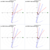 |
Fig. 1 Position of PSP (red circle) and STEREO-A (blue circle) in the ecliptic plane during the first CME (upper row) and second CME (lower row). The gray region represents CME #1 (upper row) and CME #2 (lower row) using positions calculated in Sects. 4.1 and 4.2 (Tables 2 and 4) and widths fromSect. 4.6. The Sun and Earth’s positions are represented by the orange and green circles, respectively.Left panels (a and c): first observation of each CME in WISPR-I FOV, and right: last observation on HI-1. The approximate FOV of HI-1 and WISPR-I are represented by the red and blue lines, respectively. The dashed line represents the spacecraft position in an arbitrary future point in its orbit. |
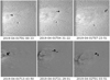 |
Fig. 2 Coronal mass ejection observed on April 1, 2019 by the WISPR-I (upper row) imager onboard PSP and HI-1 onboard STEREO-A (lower row). Here, we display only three observations for each instrument, one close to the first observation (left column), another close to the center of the observation period (center column), and another close to the last observation (right column). All images shown here are running differences, and they are cropped to highlight the CME region. The six black squares in each frame represent the CME front point selected in each visual inspection (see details in Sect. 3). |
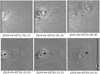 |
Fig. 3 Coronal mass ejections observed on April 2, 2019 by the WISPR-I (upper row) imager onboard PSP and HI-1 onboard STEREO-A (lower row). Here we display only three observations for each instrument, one close to the first observation (left column), another close to the center of the observation period (center column), and another close to the last observation (right column). All images shown here are running differences, and they are cropped to evidence the CME region. The six black squares in each frame represent the CME front point selected in each visual inspection (see details in Sect. 3). |
3.1 The residual of the fit and error estimation for each parameter
We extracted six time profiles of βobs and γobs by tracking the CME front six times. For each tracking attempt and fit case, we derived a set of CME kinematics parameters (ϕ2 [t0], σ2, v0, a, r2 (t0), and  ). For each fit case, we adopted the median of each parameter as our result and the standard deviation as an estimate of error. We followed the same procedure for all results reported here.
We show βobs, γobs, βder, and γder for CME #2 in Fig. 5 for a fit case using a constant speed and no deflection. Overall, median values of βder and γder (black lines) follow the observation (βobs, γobs, red lines) both in WISPR-I and HI-1 observations. The highest discrepancy |βobs − βder| is ~ 1° in the first WISPR-I measurement. The error bars for observed and derived angles have similar sizes, suggesting that the model reproduces the observations reasonably well.
One difference between the two instruments is in the angular range: βobs [tn] − βobs[t1] and γobs [tn] − γobs[t1] are both higher for WISPR-I (left panels in Fig. 5). This can be explained by the wider WISPR-I FOV (40°) when compared to HI-1 (20°). Another reason can be the difference in the spacecraft-CME distance, which is significantly smaller for PSP as the spacecraft is closer to the Sun and, therefore, to the CME.
We can also notice that the error bars in HI-1 observations (red bars in Fig. 5, right panels) clearly increase with time. At the last time-instance, they are approximately two times higher than in the first one. As the error bars result from visual inspections performed multiple times, and the CME is typically observed more clearly in the earlier measurements, βobs and γobs change less from one visual inspection to another. On the other hand, this trend is not clear on the WISPR-I observations used here. One possible explanation is that this is not a function of the spacecraft or instrument, as the results suggest, but rather of the particularities of the CME front, which can differ from one event to another.
For both CMEs and regardless of the set of free parameters used, we fit residuals σ <0.1° using observations from HI-1 and σ < 0.5° from WISPR-I. This difference can probably be explained by the different ranges of β and γ, which are proportionally higher in WISPR-I.
3.2 Multiple spacecraft fit
In the fit done in Sect. 3, we calculated the CME kinematics independently for each imager. Thus, the CME front position r2 can be different when comparing HI-1 and WISPR-I at a specific time. As there is no overlap with other CMEs, we investigate the value of a fit that forces the CME front position as a function of time r2 (t) to be the same for both heliospheric imagers.
We used all measurements available: either when the CME is visible in one FOV only or both. It is important to note that  is no longer a free parameter. Hence we have onlyfive free parameters: r2[t0], v, a, ϕ2, and σ2. The first three parameters are identical in spacecraft-specific coordinates (Fig. 4), regardless of the spacecraft considered; r2 [t] is constrained for both spacecraft. As in Sect. 3, here r2[t] is described by a second order fit (Eq. (1)). The longitude and latitude parameters (ϕ2 and σ2) are given in the spacecraft coordinate system, and we converted them from one spacecraft to the other, as described in Appendix A.
We used an extensive range for all five parameters (r2[t0], v0, a, ϕ2 [t0], and σ2) in Eqs. (3) and (4) and derived βder[t] and γder[t]. We calculated the residual of the fit σ using the following equation:
![\begin{align*} \sigma =&\, \sum_{t=1}^{m}(|\beta_{\textrm{obs}}^{\textrm{WISPR}}[t]-\beta_{\textrm{der}}^{\textrm{WISPR}}[t]|/m+|\gamma_{\textrm{obs}}^{\textrm{WISPR}}[t]-\gamma_{\textrm{der}}^{\textrm{WISPR}}[t]|/m)\ \nonumber\\ &+\sum_{t=1}^{n}(|\beta_{\textrm{obs}}^{\textrm{HI}}[t]-\beta_{\textrm{der}}^{\textrm{HI}}[t]|/n+|\gamma_{\textrm{obs}}^{\textrm{HI}}[t]-\gamma_{\textrm{der}}^{\textrm{HI}}[t]|/n),\end{align*}](/articles/aa/full_html/2021/06/aa39490-20/aa39490-20-eq13.png) (6)
(6)
where  ,
,  ,
,  , and
, and  are the angular values in each spacecraft FOV calculated using Eqs. (3) and (4), n and m are the number of measurements in WISPR-I and HI-1, respectively. It is important to notice that this equation is the sum of the residuals associated with each spacecraft.
One advantage of this methodology is that it increases the number of measurements available for the fit. This allowed us to derive the CME kinematics over a longer period, when compared to single telescope measurements. We expect reduced fit errors as more measurements are available and the number of free parameters remains the same.
On the other hand, this method can lead to inconsistencies if the specific feature tracked by βobs and γobs is not the same in both instruments. This can occur, for example, when we observe many CMEs in close timing. In this case, the association of the CME projection from one heliospheric imager to the other is ambiguous.
Hereafter, we refer to the fit introduced in this section as the multiple spacecraft fit (MSF). The cases which have observationsof one spacecraft are referred to as single spacecraft fits (SSFs).
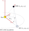 |
Fig. 4 CME front position (r2[t], ϕ2, σ2) determination using spacecraft observations (PSP or STEREO-A) from coordinates (r1, ϕ1, 0). We determined the CME kinematics by extracting the angles β and γ, knowing the spacecraft position, and assuming some constraints for the CME (such as a fixed angle or constant speed). Because of space constraints, we display ϕ2 − ϕ1 as ϕ21. |
4 Results and discussion
4.1 CME #1
CME #1 was observed and tracked for over 6 h in WISPR-I FOV and over 10 h in HI-1 FOV. The results for the SSFs and MSF are summarized in Tables 1 and 2, respectively. We illustrate the propagation direction and positions calculated using MSF in Figs. 1a and b.
In all cases, the results revealed a slow CME with speeds in the 200−300 km s−1 range, propagating 5− 8° above the ecliptic plane, and between 47° and 79° eastward of the Sun-Earth line (HCI longitudes ranging from 36° to 69°). For the SSF cases with acceleration a as a free parameter (Table 1, third column), we derived positive accelerations in both telescopes. However, this is a marginal result since the accelerations are of the same order as their errors. The MSF (Table 2) resulted in a slightly stronger indication of acceleration (0.556 ± 0.351 m s−2).
The CME front positions r2[t] derived using SSFs are shown in Fig. 6. The three upper panels show the results under three different sets of free parameters. The bottom panel compares all three fits. For each instrument, r2 [t] differences between the three cases are smaller than the error bars. So, the determination of the CME front distance is not significantly affected by the set of free parameters used, particularly acceleration and deflection that are not free parameters in all fits. We also found that the MSF r2 agrees with those results from SSF, particularly in the first WISPR-I and last HI-1 measurements.
To better evaluate the differences between WISPR-I and HI-1 SSFs, we extrapolated the WISPR-I r2 20 h ahead to compare it against HI-1 r2[t]. In all cases, the extrapolated WISPR r2 is ~ 0.05 au further away than the HI-1 r2. This suggests that there is an r2 discrepancy because of the specific feature tracked in HI-1 and WISPR-I rather than the assumptions for the fit, such as a constant speed or propagation direction. In other words, the WISPR-I feature may be a more distinct feature than the one in HI-1. There could be several reasons for this discrepancy. One reason may be that HI-1 is located further from WISPR-I and it observes the event later than WISPR-I. Other possible reasons are the CME evolution and Thompson scattering effects.
In the case that considers  as a free parameter, the resulting deflections are marginal (
 for WISPR-I and
  for HI-1). These
  errors are unsurprising as the total deflection
  (see Eq. (2)) is smaller than the longitude error. For WISPR-I,
  while the longitude error is 10°. For HI-1,
  while the longitude error is 24°. More robustdeflection estimates require a fit using longer periods.
To check whether these results were plausible, we searched for the source region of CME #1. Given the low speed and solar minimum phase, it was unsurprising to see that there were no obvious low corona signatures associated with this CME. This event was, in other words, a “stealth” CME (Robbrecht et al. 2009). In our experience, however, a careful inspection of extreme ultraviolet (EUV) images at different wavelengths and viewpoints can usually reveal the source regions, via the identification of tell-tale signs, such as widespread heating fronts or distant brightenings and slow rising loop systems. In this case, we identified the source region as an extended filament channel in the northwestern quadrant of the AIA (Atmospheric Imaging Assembly from the Solar Dynamics Observatory - SDO) image (Fig. 7). Because of the slow evolution of the eruption, it is difficult to pinpoint the exact time, but the rise started on March 29, 2019. On April 1, 2019, we detected diffuse brightentings along the channel in STEREO-A Extreme UltraViolet Imager (EUVI) images extending from 20− 40° longitude, corresponding to 38°−58° HCI longitudes. The close agreement between CME #1 and source longitudes gives us confidence as to our measurement technique.
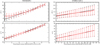 |
Fig. 5 Comparison of the observed and calculated β and γ parameters as a function of time for the CME #2 using observations from WISPR-I (left panels) and HI-1 (right panels). The lines represent the median values, and the error bars correspond to the standard deviation calculated by repeating the fit with multiple sets of observations. The red lines indicate observations, and the black lines represent values calculated by the fit. |
Kinematics parameters derived for CME #1 considering three different cases of free parameters (shown in columns).
4.2 CME #2
CME #2 was observed for approximately 16 h when combining observations from WISPR-I and HI-1. Results from the three SSF cases (( , a = 0), (
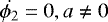 ), and (
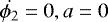 )) are shown in Table 3. For this CME, we added another variation of the fit using both instruments, but only in the 4-h period of overlapping observations. These results are shown in Table 3 in rows indicated by “both”. MSF results are shown in Table 4 and illustrated in Fig. 1 (panels “c” and “d”).
We found speeds of ~300 km s−1 with differences among the SSF cases, mostly below 50 km s−1. Regardless of the SSF, the HI-1 speed is higher than the WISPR-I speed. The difference ranges from 20 to 60 km s−1. Since the HI-1 observations occurred after the WISPR-I observations, we interpret this as a possible positive acceleration. The MSF also suggests acceleration, with speeds increasing at 157 km s−1 between the first and last observations, which were approximately 17 h apart.
Moreover, we derived significant accelerations for WISPR-I SSF (6.667 ± 2.714 m s−2) and MSF (2.778 ± 1.152 m s−2). We believe the differences in the acceleration magnitude can be explained by timing: The last time-instance tf used on MSF was ~18 h later than in the WISPR-I SSF.
For all fit cases, the propagation direction is above the ecliptic plane (~ 10°) and eastward from Earth (westward from STEREO-A). The HEE longitudes are − 21° to − 61°, depending on the SSF fit. It is interesting to note that the latitude and longitude errors (4° and 1°, respectively) are clearly lower in the fit with simultaneous observations (rows labeled “both” in Table 3) and in the MSF (Table 4).
Regardless of the fit, the CME latitude and longitude derived from WISPR-I observations are higher than those derived from HI-1 (Table 3). A likely reason for this discrepancy is the specific feature tracked. Although we tried to identify the same feature on both instruments, the association is subjective since the CME projection in each image is considerably different, particularly because of the different distances from the observing spacecraft, as we have discussed for CME #1.
The longitudinal deflection fit indicates that CME #2 is deflecting westward. We found  to be equal to 0.4 − 0.8° h−1 with errors of 0.2−0.3° h−1. This deflection magnitude is similar to the solar rotation speed (~ 0.5° h−1) and indicates that the CME is corotating with the Sun.
We compare the CME position r2[t] in WISPR-Iand HI-1 in Fig. 8. In the period with simultaneous observations, r2 [t] from WISPR-I is similar to r2[t] from HI-1 only in the SSF in which acceleration was a free parameter (Fig. 8, third panel from top). This suggests that the error of this fit is quite small as r2 is calculatedindependently for each spacecraft. In the remaining cases, the results are considerably different. The position of HI-1 is further away from the Sun ~0.02 au (red and green curves), which is similar or higher than the error bars. When we compare all SSFs in each instrument FOV (bottom panel in Fig. 8), the maximum difference in the position is ~ 0.02 au for WISPR-I and ~0.05 for HI-1.
The kinematics of CME #2 using WISPR-I observations are also reported in Liewer et al. (2020). The authors used a methodology based on Liewer et al. (2019), which considers the same geometrical determination of the CME front shown in Fig. 4 and resembles the SSF case without acceleration or deflection. One major difference with our study is that we tracked the CME outermost point in the front, while Liewer et al. (2020) tracked the lower dark “eye” of the skull-like flux rope, which is located closer to the Sun in a more central CME region. Thus, differences in the results are expected, as different features within the same CME may exhibit different motion patterns.
Liewer et al. (2020) found the CME position to be ~0.06 au on April 2, 2019 at 12:09 UT. The position we derived for the same time is further away from the Sun (see Fig. 6). This difference is consistent with the points tracked, since we were following a CME feature that is further away from the Sun.
The HCI longitude ranges from 56° to 95°, which encompasses the result from Liewer et al. (2020) (= 67 ± 1°). The same HCI longitude was found by Liewer et al. (2020) for the source region of this CME, identified to be AR12737, at its eruption time (March 31, 2019 at approximately 13 UTC). The same holds for the speeds. Our results (260 km s−1 to 381 km s−1) encompass the Liewer et al. (2020) result (333 ± 1 km s−1).
One major difference between our results and Liewer et al. (2020) is the error range that each parameter has. Regarding the speed, the errors found here range from 17 to 33 km s−1, considering only the results from the WISPR-I observations, and from 13 to 82 km s−1, considering both spacecrafts. As for the longitude, our errors range from 1° to 14°, while in Liewer et al. (2020) the longitudinal error is 1°. We believe that the way we calculated this error explains this difference. We have six time-series of (βobs[t], γobs[t]), which were derived from six independent trackings. In each time-series, we calculated the kinematics using our fit method. We then derived the error as 1-σ between the six sets of kinematic parameters. Liewer et al. (2020) derived β and γ measurements from three independent trackings and then calculated the mean value for each time. Using the mean time-series mean as input, the CME kinematic parameters (speed, position, longitude, and latitude) were found using Levenberg-Marquardt least-squares. The uncertainty considered is a 1-σ error from the fit procedure. Overall, our results are consistent with those from Liewer et al. (2020).
Kinematics parameters derived for CME #1 using the fit with observations from both spacecrafts.
 |
Fig. 6 CME #1 position r2[t] derived by SSFs. The continuous lines show the median values, and the error bars indicate the minimum and maximum values. Each color represents a fit with a different set of free parameters, which is indicated in each panel. All plots shown in the three upper panels are repeated in the bottom one to help compare the fits. The results from MSF are not shown. |
 |
Fig. 7 CME #1 source region in AIA 304 Å (left) and EUVI-A 195 Å/304 Å composite (right). |
CME #2 derived kinematics considering three different cases of free parameters (shown in columns).
CME #2 kinematics derived with the observations from both spacecrafts.
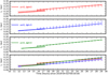 |
Fig. 8 CME #2 position r2[t] derived by SSFs. The continuous lines show the median values, and the error bars indicate the minimum and maximum values. Each color represents a fit with a different set of free parameters, which is indicated in each panel. All plots shown in the three upper panels are repeated in the bottom panel to help compare the fits. The results from MSF are not shown. |
4.3 How the errors compare between WISPR-I and HI-1
The SSF results from WISPR-I have lower errors for CME #1, but higher errors for CME #2. This trend is the same for all parameters studied here: distance, speed, acceleration, latitude, longitude, and deflection. The only exception is the CME #2 speed in one SSF case.
We calculated the errors from the multiple, visual identification of the CME front, that is, from the different βobs[t] and γobs[t] used in each fit. As the CME front identification is somehow subjective, we believe that the differences between the WISPR-I and HI-1 results are due to the feature selection.
4.4 Comparing the fit with multiple and single spacecraft observations
In this section, we compare MSFs (Tables 2 and 4) with SSFs (Tables 1 and 3). For the latter, we chose the case that uses the acceleration as a free parameter, but does not consider deflection (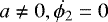 ), as this case has the same free parameters as the MSF.
For both CMEs, the discrepancies in distance r2 and speed at t0 are smaller than the errors. On the other hand, discrepancies exceed the errors for longitudes, CME #2 acceleration, and HI-1 latitudes. We also noticed that when we compared HI-1 and WISPR-I SSFs, the same parameters had discrepancies that exceed the errors bars. Thus, MSF particularities, such as the position constraint from one spacecraft to the other, are unlikely to be the major explanation for the discrepancies, as we also observed them when we compare SSFs from different instruments.
Regarding errors, the MSF errors have lower values for many parameters: the longitude (1− 3° when compared to4−10° from SSFs), r2[tf] (~ 0.01 au rather than ~ 0.05 au), and the speed at t0 (10−40 km s−1 when compared to13−82 km s−1). There is no clear trend for latitude or acceleration.
The lower errors of the MSF kinematic parameters possibly result from the higher number of measurements available: 38 for CME #1 and 37 for CME #2. It is important to notice that MSF measurements correspond to the sum of those available on the HI-1 and WISPR-I SSFs (m + n on Eq. (6)).
4.5 The Thomson sphere and its effect on the longitude
The tangent to the Sun of an observer’s line of sight (LOS) for a particular elongation lies on the Thomson sphere (TS; Vourlidas & Howard 2006). The tangent point marks the location where the Thomson scattered emission from the free CME electrons in the corona is maximum along that LOS. This diameter of the sphere is equal to the Sun-observer distance. Features contribute progressively less to the LOS emission as their angular distance from the TS increases (see details in Vourlidas & Howard 2006).
Because of PSP’s proximity to the Sun, the TS diameter for the WISPR observations is about four times smaller than for STEREO-A/HI-1. Since the two telescopes were approximately radially aligned when they observed the two CMEs, WISPR would be more sensitive to material closer to the spacecraft and hence would image the eastward flanks of the CME, that is to say relative to Earth. Also, the WISPR LOS is much narrower than the HI-1 LOS and hence more sensitive to small-scale structures. Thus, we expect the CME propagation direction derived from WISPR observations to be eastward of the HI-1 estimates. The longitudinal differences between WISPR and HI-1 for CME #1 (all three cases of free parameters, Table 1) are in agreement with this expectation. The opposite trend for CME #2 (Table 3).
Errors in the longitudinal fits are in opposite directions in the two CMEs studied here. This suggests that the TS effect is not the dominant source of longitude discrepancies for CME #2. With the derived kinematics, though, it is not possible to state which is the primary reason for the CME #1 discrepancy. The TS effect could be a source. It is possible that the specific features tracked in each instrument may lie behind the differences in the derived longitude for CME #2 and perhaps for CME #1.
4.6 CME widths
The CME width is necessary for determining whether a CME intersects at a location where in situ measurements are available. As a first order approximation, we considered the CME angular extent in latitude to be equal to the longitudinal one. As the latitude errors are lower (≤ 3°) than the longitudinal ones (≤24°), we estimated the latitudinal angular extent. To do so, we tracked the lowermost and utmost CME features as observed by WISPR-I, which correspond to the southern and northernmost CME portions. Here we repeated the same methodology used to calculate the CME front (Sect. 3) with the same set of WISPR-I images.
The angular extent we found here using WISPR-I observations are 13° for CME #1 and 16° for CME #2. To estimate the uncertainty of these angles, we repeated the fit using different sets of free parameters (Sect. 3) and six sets of CME features identified from visual inspection in both the utmost and lowest CME features. We found a standard deviation of 3°.
We measured a ~20° width for both CMEs in the HI-1 observations, which is a few degrees wider than WISPR-I measurements. We could not account for the difference so the CME is likely expanding or the longer HI1 LOS reveals a fainter structure around the CME.
We realized that the CME #2 studied here is included in the HELiospheric Cataloguing, Analysis, and Techniques Service (HELCATS) project1. According to this catalog, the CME #2 angular width is 20°, which is similar to our results.
4.7 Exposure time
The exposure time is an important difference between the HI-1 and WISPR-I observations. It is 25.6s for WISPR-I versus 20 min for HI-1, which translates to a radial motion of 0.5 solar radii (or 8 HI-1 pixels) for the derived speeds. This distance is much smaller thanthe position discrepancies (Figs. 6 and 8), which are approximately one order of magnitude larger (~5 solar radii).
The CME motion during the HI-1 exposure results in a positional uncertainty of 2° in longitude and less than 1° in latitude. These error estimates are based on the viewing angle, position, speed, and propagation direction, and they are smaller than the error estimates in Tables 1 and 3.
Hence, the difference in exposure times is unlikely to significantly affect the derivation of positions in the two CMEs. However, the differentexposure times could have important effects for fast CMEs. For example, CMEs with speeds above 1200 km s−1 travel more than 2 solar radii within an HI-1 exposure, which translates to over 30 HI-1 pixels.
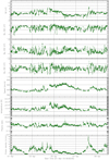 |
Fig. 9 Interplanetary magnetic field magnitude, orthogonal components, and solar wind parameters (proton density, proton speed, temperature) as well as the plasma beta parameter observed near Earth. |
5 In situ observation
We now check whether any of the CMEs were observed in situ, either in the Earth’s vicinity (Sect. 5.1) or by PSP (Sect. 5.2). The objective is to see if the in situ measurements are consistent with the kinematics we derived in Sects. 4.1 and 4.2, particularly the propagation directions.
5.1 Near Earth in situ observation
The interplanetary in situ magnetic field and solar wind parameters observed close to the Earth are shown in Fig. 9. The panels, from top to bottom, show: (i) the magnetic field intensity; (ii–iv) its orthogonal components (given in geocentric earth-ecliptic coordinates – GSE); (v) the solar wind proton bulk speed; (vi) the proton temperature; (vii) the plasma beta parameter, which is the ratio between the plasma and magnetic pressures; and (viii) the proton density. The data shown here were merged by King & Papitashvili (2005) from two spacecrafts located close to Earth: Advanced Composition Explorer (ACE; Stone et al. 1998), particularly from the magnetic field instrument (MAG; Smith et al. 1998)and the Solar Wind Electron, Proton, and Alpha Monitor (SWEPAM; McComas et al. 1998), as well as Wind’s Magnetic Field Instrument (MFI; Lepping et al. 1995) and Solar Wind Experiment (SWE; Ogilvie et al. 1995).
The observed interplanetary signatures are inconsistent with the expected signatures from a typical CME: (i) the peak magnetic field intensities do not exceed 9 nT. This is among the lowest values observed (see, e.g., Richardson & Cane 2010); (ii) the interplanetary magnetic field does not have a clear rotation; (iii) the plasma beta parameter is higher than 1 in almost any period after the peaks in the magnetic field intensity; (iv) the magnetic field variance does not decrease in the period with an enhanced magnetic field. Normally higher fluctuations are observed in the period ahead of interplanetary CMEs.
We can interpret these signatures as one of the following possibilities: (i) a disturbance possibly associated with the CME but not the flux rope itself, such as the sheath region; (ii) a flux rope portion far from its center, which does not produce a clear field rotation in the magnetic field components observed by a spacecraft crossing the structure; or (iii) a streaming interaction region, which is an interplanetary structure formed by the interaction of a slow wind stream followed by a fast one (see, e.g., Richardson 2018, and references therein). These regions are associated with increased interplanetary magnetic fields.
This is in agreement with the CME propagation directions, which show both CMEs located eastward from the Sun-Earth line (Tables 1–4). The CME longitudinal angle with the Sun-Earth line ranges from 47 ± 24° to 79 ± 7° for #1 and from 21 ± 10° to 61 ± 8° for #2, depending on the fit used. For both CMEs, the result for all fits indicate that the propagation direction of the CME longitude is eastward from the Earth (gray region in Fig. 1). Since the longitudinal width of the CMEs is rather small (< 20°), it is unlikely they intercepted Earth.
5.2 PSP in situ observation
The CME #1 front was in an appropriate solar distance to reach PSP (r2 ~ 0.2 au) in the first hours of April 2, 2019 (Figs. 1b and 6), when the spacecraft HCI longitude was ~ 20°. When the CME #1 HCI longitude is between 36 ± 7° and 69 ± 9°, depending on the fit method considered, it is clearly westward from PSP and we do not expect it in situ.
Performing a similar analysis, we found that CME #2 is also westward from PSP. This CME solar distance was equal to PSP’s in the first hours of April 3, 2019 (Figs. 1d and 8). At this time, the CME HCI longitude was between 56 ± 8° and 95 ± 10° and PSP’s was ~40°.
We also calculated the moment that PSP and each CME became longitudinally aligned. We used the longitude from MSF as the central longitude and the longitudinal width calculated in Sect. 4.6. This took place at April 3, 2019 12:00 UT for CME #1 and at April 4, 2019 18:00 UT for CME #2. We estimated an error of approximately 3 h in the arrival time considering the width error (approximately 3°). Therefore, PSP is likely to have crossed the wakes of both CMEs.
We show the PSP in situ measurements in Fig. 10. From top to bottom, the panels show the magnetic field intensity, itsorthogonal components (radial, tangential, and normal), the solar wind proton speed, and density. Each panel shows 1-min medians. In the two bottom panels, we use level 3 solar wind bulk parameters (density and speed) from the Solar Probe Cup (SPC), which is part of the Solar Wind Electrons Alphas and Protons (SWEAP) instrument suite (Kasper et al. 2016; Case et al. 2020)onboard PSP. SPC is a Faraday Cup that looks directly to the Sun and measures ion and electron fluxes and flow angles as a function of energy. The measurements from this instrument are not obscured by the PSP heat shield. The magnetic field data shown in the four upper panels are level 2 from FIELDS instrument (Bale et al. 2016). The magnetic field, its orthogonal components, and the solar wind density were normalized by the square of the PSP distance. For all parameters, we used the position of PSP on April 1, 2019 at 0:00 UT as a reference point in the normalization.
The in situ measurements shown in Fig. 10 are studied in Rouillard et al. (2020). They interpreted the region with a lowerdensity observed from April 3 to 7, 2019, except for a brief period on April 6, 2019 when PSP was leaving the streamer belt flows.
The interplanetary magnetic field lacks typical signatures of in situ measurements of CMEs, such as a higher magnetic field with rotation and low plasma density (see, e.g., Zurbuchen & Richardson 2006; Richardson & Cane 2010). Thus, the PSP in situ measurements indicate that PSP crosses behind the CMEs and agree with our results about the CME propagation direction. Whether these observations reveal any information about the post-CME flow will require a more detailed study.
 |
Fig. 10 Magnetic field magnitude, orthogonal components (radial, tangential, and normal), and solar wind proton parameters (proton speed and density) observed in situ on PSP from April 1 to 10, 2019. The magnetic field and solar wind protondensity were normalized by the square of PSP’s solar distance. |
6 Final remarks
We derived the kinematics of CMEs #1 and #2 (April 1 and 2, 2019) using observations from two vantage points. The novelty here is that the observations were along similar angular distances from the CME, but from very different heliocentric distances (0.96 for HI-1, 0.19 au for WISPR).
We introduced a new method to derive the CME propagation using observations from both viewpoints as constraints. This is based on the position determination introduced by Liewer et al. (2019), which is suitable for the fast changes in the PSP longitude. This methodology adds CME acceleration and deflection as free parameters, along with speed, position, longitude, and latitude. Considering the HI-1 and WISPR-I observations (both combined independently) and by performing a fit, we determined the CMEs kinematics in solar distances between ~ 0.1 and ~ 0.2 au.
Our findings are summarized as follows:
- 1.
Both CMEs are slow (200−274 km s−1 for #1 and 260−432 km s−1 for #2) and propagate northward from the ecliptic plane (5−8° for #1 and 6−19° for #2).
- 2.
For CME #2, the speed is higher on HI-1 FOV than on WISPR-I FOV. Depending on the SSF, the differences range from 20 to 60 km s−1 and they are higher than or equal to the speed errors estimated here. Since HI-1 observes the CME further from the Sun (start at ~0.1 au), CME #2 may be accelerating. This agrees with SSFs that had acceleration as a free parameter, which also resulted in positive values for this parameter. The MSF acceleration is also positive, with the speed increasing from 275 to 432 km s−1 while the CME propagates from 0.08 to 0.22 au. For CME #1, we also found acceleration, but the magnitude is the same order as the error, so it is a marginal result.
- 3.
Both CMEs propagate eastward from Earth and westward from PSP and STEREO-A. Depending on the fit case considered, their angular distance with Earth is between 47° and 79° for CME #1, and between 21° and 61° for CME #2. The longitudinal differences remain whether we compare cases of SSFs with different free parameters or SSFs from different instruments. Thus, the discrepancies in the longitude are unlikely to be due to the instrument or the set of free parameters. We understand that the difference in the CME longitude from one method to the other is a combination of the error from tracking different CME front features on HI-1 and WISPR-I.
- 4.
To assess the errors in our kinematic results, we visually tracked and fitted the CME front several times. We then used the spread in the resulting kinematic parameters to derive the error estimates of up to ~0.05 au in radial distance, ~10° in latitude, and ~24° in longitude. These errors cannot fully explain the discrepancies in the position and direction of propagation found when comparing the results from HI-1 and WISPR-I. The most likely explanation is that we are not tracking the same feature in both telescopes.
- 5.
Fits with WISPR-I observations result in lower errors for CME #1 but higher errors for CME #2 when compared to those from HI-1. Thus, we do not see any clear trend of smaller fit errors in any instrument or spacecraft.
- 6.
We allowed CME longitudinal deflection as a free parameter in the fit. For CME #2, we found significant westward deflections for both WISPR-I and HI-1 SSFs. The longitudinal deflection magnitude is consistent with the solar rotation, and we believe that this is an indication that CME #2 is corotating with the Sun up to ~0.2 au. The deflection estimates for CME #1 are smaller than their errors.
- 7.
Thomson scattering considerations suggest that WISPR-I estimates should be based eastward of HI-1 estimates if Thomson scattering effects were important. We found this trend for CME #1 (April 1), but not for CME #2 (April 2). For the latter, the longitudes derived using the WISPR-I observations are more than 13° westward compared to HI-1 observations. A plausible explanation for this difference is that the specific features tracked are different in each instrument’s FOV and this affects the derived longitudes more than the Thomson scattering.
- 8.
The MSF has lower errors for the position, speed, and longitude. One possible explanation is the higher number of measurements available when compared to the SSF. For the remaining parameters, there is no clear trend.
- 9.
The positions and speeds derived using the MSF agree with those derived using SSFs. Acceleration, longitude, and latitude have discrepancies between corresponding HI-1 and WISPR-I SSFs and also when we compared MSF with a SSF.
- 10.
We inspected in situ measurements from PSP and the near-Earth spacecraft and found no clear signatures of interplanetary counterparts of any CME studied here. This finding supports the CME propagation directions from both MSF and SSFs.
In future studies, we plan to apply the methodology discussed here to other CMEs observed both by PSP and STEREO-A. In particular, this study can be applied to events with in situ measurements close to the Sun by PSP.
Acknowledgements
C.R.B. acknowledges the support from the NASA STEREO/SECCHI (NNG17PP27I) program. A.V. is supported by the WISPR Phase-E funding and NASA 80NSSC19K1261 grant. Parker Solar Probe was designed, built, and is now operated by the Johns Hopkins Applied Physics Laboratory as part of NASA’s Living with a Star (LWS) program (contract NNN06AA01C). Support from the LWS management and technical team has played a critical role in the success of the Parker Solar Probe mission. The Wide-Field Imager for Parker Solar Probe (WISPR) instrument was designed, built, and is now operated by the US Naval Research Laboratory in collaboration with Johns Hopkins University/Applied Physics Laboratory, California Institute of Technology/Jet Propulsion Laboratory, University of Gottingen, Germany, Centre Spatiale de Liege, Belgium and University of Toulouse/Research Institute in Astrophysics and Planetology. WISPR data are available for download at https://wispr.nrl.navy.mil/. We acknowledge the NASA Parker Solar Probe Mission and the SWEAP team led by J. Kasper for use of data. SWEAP data are available at http://sweap.cfa.harvard.edu/. The FIELDS experiment on the Parker Solar Probe spacecraft was designed and developed under NASA contract NNN06AA01C. FIEDLS data can be downloaded at https://fields.ssl.berkeley.edu/. The Sun Earth Connection Coronal and Heliospheric Investigation (SECCHI) was produced by an international consortium of the Naval Research Laboratory (USA), Lockheed Martin Solar and Astrophysics Lab (USA), NASA Goddard Space Flight Center (USA), Rutherford Appleton Laboratory (UK), University of Birmingham (UK), Max Planck Institute for Solar System Research (Germany), Centre Spatiale de Liége (Belgium), Institut d’Optique Theorique et Appliquée (France), and Institut d’Astrophysique Spatiale (France). STEREO/SECCHI data are available for download at https://secchi.nrl.navy.mil/. We acknowledge use of NASA/GSFC’s Space Physics Data Facility’s CDAWeb service, and OMNI data. This data is available for download at https://omniweb.sci.gsfc.nasa.gov/html/ow_data.htm. This research has made use of the Solar Wind Experiment (SWE) and Magnetic Field Investigations (MFI) instrument’s data onboard WIND. We thank to the Wind team and the NASA/GSFC’s Space Physics Data Facility’s CDAWeb service to make the data available. Wind data are available from https://cdaweb.sci.gsfc.nasa.gov. We thank P. C. Liewer and J. Qiu for useful discussions.
Appendix A Coordinate conversion from and to spacecraft orbit
Examples of coordinate systems commonly adopted by the heliophysics community are the Heliocentric Earth EQuatorial (HEEQ; Hapgood 1992), the Heliocentric Earth Inertial (HCI; Burlaga 1984), and Carrington, which are based on the solar equatorial plane, as well as the Heliospheric Earth Ecliptic (HEE; Hapgood 1992), based on the ecliptic plane. For a complete explanation about all of these coordinate systems, readers are referred to Thompson (2006).
The coordinate system used here to derive the CME position (Fig. 4) is not frequently used. It is heliocentric, and its x and y axes are in the spacecraft orbit. Neither PSP nor STEREO orbits lie in or are parallel to the solar equatorial or the ecliptic plane.
We call the coordinate system used in Fig. 4 the heliocentric spacecraft orbital (HSO). Its x points from the Sun to the spacecraft position, z is perpendicular to the orbit plane, and y lies in the orbit plane and forms the orthogonal right-handed coordinate system. In the case of STEREO-Aand PSP, whose orbits are both counterclockwise from an observed located in the north, the y corresponds to a future position in the orbit. It is important to notice that this coordinate system is spacecraft specific and all axes change as the spacecraft orbits the Sun. For PSP, the x and y axes change tents of degrees in a matter of days, particularly close to the perihelium.
In order to compare the CME position for PSP and STEREO-A, we need to convert them to a common coordinate system, such as HEEQ or HEE. Both the x axes follow the Earth’s position around the Sun and they are not inertial for a given CME. Instead, we used the HCI coordinates, which do not follow the solar rotation nor the Earth’s rotation around the Sun. The HCI x-axis is the solar ascending node on the ecliptic of J2000.0, the z axis is perpendicular to the solar equatorial plane, and y is also in the solar equatorial plane and forms the right-handed coordinate system.
A given position vector r can be written in both HSO (o) and HCI (i) coordinate systems:
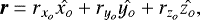 (A.1)
(A.1)
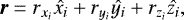 (A.2)
(A.2)
where  , and
, and  are unit vectors in the HSO coordinate system and
  , and
, and  are in the HCI.
By multiplying Eq. (A.1) by  ,
,  , and
, and  , we get:
 (A.3)
(A.3)
 (A.4)
(A.4)
 (A.5)
(A.5)
which can be written in the following matrix form:
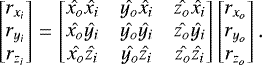 (A.6)
(A.6)
By definition, 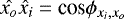 where
where  is the angle between the unit vectors. It is important to notice that
  depends only on the two coordinate systems used and is identical for any vector used. The same conclusion can be derived for any elements from this matrix. This matrix transforms any vector from o coordinates to i coordinates and hereafter we refer to it as To2i. Thus, we can rewrite Eq. (A.6) as:
 (A.7)
(A.7)
Multiplying by the inverse matrix of To2i on both the right- and left-hand side results in the following:
 (A.8)
(A.8)
Hereafter, we refer to  as Ti2o.
We need to find the CME position in HCI coordinates Ri and we have Ro. To do so, we need to know the transformation matrices To2i. It is important to notice that since the HSO coordinate system is rotating to follow the spacecraft position and changes as a function of time, the transformation matrices To2i and Ti2o need to be calculated for each time instance and for each spacecraft.
We can calculate the elements of the first row of To2i ( ) by using
  , where
  is the unit vector pointing from the Sun to the spacecraft location, that is, the x axis in the HCO coordinate system. Thus, we can write:
 (A.10)
The HCI coordinates of a ( ), which correspond to the unit vector pointing from the Sun to the spacecraft, are known and can be derived by using get_sunspice_coords.pro from SolarSoft.
Similarly, the terms in the second and third rows of To2i can be determined by having  and
and  . HCI components of
  can be derived by the cross product of
  at two different measurements and
  is found by
  .
.
By doing so, we have determined the transformation matrix To2i. Thus, we can convert the CME position vector from HSO coordinates, which are spacecraft and time specific, to HCI coordinates, which are inertial and can be easily converted to many other coordinate systems using convert_sunspice_coord.pro from SolarSoft.
References
- Bale, S. D., Goetz, K., Harvey, P. R., et al. 2016, Space Sci. Rev., 204, 49 [Google Scholar]
- Brueckner, G. E., Howard, R. A., Koomen, M. J., et al. 1995, Sol. Phys., 162, 357 [NASA ADS] [CrossRef] [Google Scholar]
- Burlaga, L. F. 1984, Space Sci. Rev., 39, 255 [Google Scholar]
- Case, A. W., Kasper, J. C., Stevens, M. L., et al. 2020, ApJS, 246, 43 [Google Scholar]
- Domingo, V., Fleck, B., & Poland, A. I. 1995, Space Sci. Rev., 72, 81 [Google Scholar]
- Fox, N. J., Velli, M. C., Bale, S. D., et al. 2016, Space Sci. Rev., 204, 7 [NASA ADS] [CrossRef] [Google Scholar]
- Freeland, S. L., & Handy, B. N. 1998, Sol. Phys., 182, 497 [NASA ADS] [CrossRef] [Google Scholar]
- Hapgood, M. A. 1992, Planet. Space Sci., 40, 711 [Google Scholar]
- Hess, P., Rouillard, A. P., Kouloumvakos, A., et al. 2020, ApJS, 246, 25 [Google Scholar]
- Howard, R. A., Moses, J. D., Vourlidas, A., et al. 2008, Space Sci. Rev., 136, 67 [NASA ADS] [CrossRef] [Google Scholar]
- Howard, R. A., Vourlidas, A., Bothmer, V., et al. 2019, Nature, 576, 232 [Google Scholar]
- Kahler, S. W., & Webb, D. F. 2007, J. Geophys. Res. Space Phys., 112, A9 [Google Scholar]
- Kaiser, M. L., Kucera, T. A., Davila, J. M., et al. 2007, Space Sci. Rev., 136, 5 [Google Scholar]
- Kasper, J. C., Abiad, R., Austin, G., et al. 2016, Space Sci. Rev., 204, 131 [NASA ADS] [CrossRef] [Google Scholar]
- King, J. H., & Papitashvili, N. E. 2005, J. Geophys. Res. Space Phys., 110, A02104 [Google Scholar]
- Lepping, R. P., Acũna, M. H., Burlaga, L. F., et al. 1995, Space Sci. Rev., 71, 207 [Google Scholar]
- Liewer, P., Vourlidas, A., Thernisien, A., et al. 2019, Sol. Phys., 294, 93 [Google Scholar]
- Liewer, P. C., Qiu, J., Hall, J. R., Vourlidas, A., & Howard, R. A. 2020, Sol. Phys., 295, 140 [Google Scholar]
- Lugaz, N., Vourlidas, A., & Roussev, I. I. 2009, Ann. Geophys., 27, 3479 [Google Scholar]
- MacQueen, R. M., Eddy, J. A., Gosling, J. T., et al. 1974, ApJ, 187, L85 [Google Scholar]
- MacQueen, R. M., Csoeke-Poeckh, A., Hildner, E., et al. 1980, Sol. Phys., 65, 91 [Google Scholar]
- McComas, D. J., Bame, S. J., Barker, P., et al. 1998, Space Sci. Rev., 86, 563 [Google Scholar]
- Ogilvie, K. W., Chornay, D. J., Fritzenreiter, R. J., et al. 1995, Space Sci. Rev., 71, 55 [NASA ADS] [CrossRef] [Google Scholar]
- Richardson, I. G. 2018, Liv. Rev. Sol. Phys., 15, 1 [Google Scholar]
- Richardson, I. G., & Cane, H. V. 2010, Sol. Phys., 264, 189 [Google Scholar]
- Robbrecht, E., Patsourakos, S., & Vourlidas, A. 2009, ApJ, 701, 283 [Google Scholar]
- Rouillard, A. P., Davies, J. A., Forsyth, R. J., et al. 2008, Geophys. Res. Lett., 35, 10 [Google Scholar]
- Rouillard, A. P., Kouloumvakos, A., Vourlidas, A., et al. 2020, ApJS, 246, 37 [Google Scholar]
- Sheeley, N. R., J., Michels, D. J., Howard, R. A., & Koomen, M. J. 1980, ApJ, 237, L99 [Google Scholar]
- Sheeley, N. R., Walters, J. H., Wang, Y.-M., & Howard, R. A. 1999, J. Geophys. Res. Space Phys., 104, 24739 [Google Scholar]
- Smith, C. W., L’Heureux, J., Ness, N. F., et al. 1998, Space Sci. Rev., 86, 613 [Google Scholar]
- Stone, E. C., Frandsen, A. M., Mewaldt, R. A., et al. 1998, Space Sci. Rev., 86, 1 [Google Scholar]
- Thompson, W. T. 2006, A&A, 449, 791 [NASA ADS] [CrossRef] [EDP Sciences] [Google Scholar]
- Tousey, R. 1973, Space Res. Conf., 2, 713 [Google Scholar]
- Vourlidas, A., & Howard, R. A. 2006, ApJ, 642, 1216 [Google Scholar]
- Vourlidas, A., Howard, R. A., Plunkett, S. P., et al. 2016, Space Sci. Rev., 204, 83 [NASA ADS] [CrossRef] [Google Scholar]
- Wood, B. E., Hess, P., Howard, R. A., Stenborg, G., & Wang, Y.-M. 2020, ApJS, 246, 28 [Google Scholar]
- Zurbuchen, T. H., & Richardson, I. G. 2006, Space Sci. Rev., 123, 31 [Google Scholar]
All Tables
Kinematics parameters derived for CME #1 considering three different cases of free parameters (shown in columns).
Kinematics parameters derived for CME #1 using the fit with observations from both spacecrafts.
CME #2 derived kinematics considering three different cases of free parameters (shown in columns).
All Figures
|
Fig. 1 Position of PSP (red circle) and STEREO-A (blue circle) in the ecliptic plane during the first CME (upper row) and second CME (lower row). The gray region represents CME #1 (upper row) and CME #2 (lower row) using positions calculated in Sects. 4.1 and 4.2 (Tables 2 and 4) and widths fromSect. 4.6. The Sun and Earth’s positions are represented by the orange and green circles, respectively.Left panels (a and c): first observation of each CME in WISPR-I FOV, and right: last observation on HI-1. The approximate FOV of HI-1 and WISPR-I are represented by the red and blue lines, respectively. The dashed line represents the spacecraft position in an arbitrary future point in its orbit. |
| In the text | |
|
Fig. 2 Coronal mass ejection observed on April 1, 2019 by the WISPR-I (upper row) imager onboard PSP and HI-1 onboard STEREO-A (lower row). Here, we display only three observations for each instrument, one close to the first observation (left column), another close to the center of the observation period (center column), and another close to the last observation (right column). All images shown here are running differences, and they are cropped to highlight the CME region. The six black squares in each frame represent the CME front point selected in each visual inspection (see details in Sect. 3). |
| In the text | |
|
Fig. 3 Coronal mass ejections observed on April 2, 2019 by the WISPR-I (upper row) imager onboard PSP and HI-1 onboard STEREO-A (lower row). Here we display only three observations for each instrument, one close to the first observation (left column), another close to the center of the observation period (center column), and another close to the last observation (right column). All images shown here are running differences, and they are cropped to evidence the CME region. The six black squares in each frame represent the CME front point selected in each visual inspection (see details in Sect. 3). |
| In the text | |
|
Fig. 4 CME front position (r2[t], ϕ2, σ2) determination using spacecraft observations (PSP or STEREO-A) from coordinates (r1, ϕ1, 0). We determined the CME kinematics by extracting the angles β and γ, knowing the spacecraft position, and assuming some constraints for the CME (such as a fixed angle or constant speed). Because of space constraints, we display ϕ2 − ϕ1 as ϕ21. |
| In the text | |
|
Fig. 5 Comparison of the observed and calculated β and γ parameters as a function of time for the CME #2 using observations from WISPR-I (left panels) and HI-1 (right panels). The lines represent the median values, and the error bars correspond to the standard deviation calculated by repeating the fit with multiple sets of observations. The red lines indicate observations, and the black lines represent values calculated by the fit. |
| In the text | |
|
Fig. 6 CME #1 position r2[t] derived by SSFs. The continuous lines show the median values, and the error bars indicate the minimum and maximum values. Each color represents a fit with a different set of free parameters, which is indicated in each panel. All plots shown in the three upper panels are repeated in the bottom one to help compare the fits. The results from MSF are not shown. |
| In the text | |
|
Fig. 7 CME #1 source region in AIA 304 Å (left) and EUVI-A 195 Å/304 Å composite (right). |
| In the text | |
|
Fig. 8 CME #2 position r2[t] derived by SSFs. The continuous lines show the median values, and the error bars indicate the minimum and maximum values. Each color represents a fit with a different set of free parameters, which is indicated in each panel. All plots shown in the three upper panels are repeated in the bottom panel to help compare the fits. The results from MSF are not shown. |
| In the text | |
|
Fig. 9 Interplanetary magnetic field magnitude, orthogonal components, and solar wind parameters (proton density, proton speed, temperature) as well as the plasma beta parameter observed near Earth. |
| In the text | |
|
Fig. 10 Magnetic field magnitude, orthogonal components (radial, tangential, and normal), and solar wind proton parameters (proton speed and density) observed in situ on PSP from April 1 to 10, 2019. The magnetic field and solar wind protondensity were normalized by the square of PSP’s solar distance. |
| In the text | |
Current usage metrics show cumulative count of Article Views (full-text article views including HTML views, PDF and ePub downloads, according to the available data) and Abstracts Views on Vision4Press platform.
Data correspond to usage on the plateform after 2015. The current usage metrics is available 48-96 hours after online publication and is updated daily on week days.
Initial download of the metrics may take a while.