| Issue |
A&A
Volume 650, June 2021
|
|
|---|---|---|
| Article Number | A88 | |
| Number of page(s) | 7 | |
| Section | The Sun and the Heliosphere | |
| DOI | https://doi.org/10.1051/0004-6361/202038082 | |
| Published online | 10 June 2021 | |
Energy partition in a confined flare with an extreme-ultraviolet late phase⋆
1
Key Laboratory of Dark Matter and Space Astronomy, Purple Mountain Observatory, CAS, Nanjing 210023, PR China
e-mail: This email address is being protected from spambots. You need JavaScript enabled to view it.
2
Key Laboratory of Planetary Sciences, Shanghai Astronomical Observatory, Shanghai 200030, PR China
3
CAS Key Laboratory of Solar Activity, National Astronomical Observatories, CAS, Beijing 100101, PR China
4
School of Astronomy and Space Science, Nanjing University, Nanjing 210023, PR China
5
State Key Laboratory of Lunar and Planetary Sciences, Macau University of Science and Technology, Macau, PR China
Received:
3
April
2020
Accepted:
8
April
2021
Abstract
Aims. In this paper, we reanalyze the M1.2 confined flare with a large extreme-ultraviolet (EUV) late phase on 2011 September 9, with a focus on its energy partition.
Methods. The flare was observed by the Atmospheric Imaging Assembly (AIA) on board the Solar Dynamics Observatory (SDO). The three-dimensional (3D) magnetic fields of the active region 11283 prior to the flare were obtained using nonlinear force free field modeling and the vector magnetograms observed by the Helioseismic and Magnetic Imager (HMI) on board the SDO. Properties of the nonthermal electrons injected into the chromosphere were obtained from the hard X-ray observations of the Ramaty Hight Energy Solar Spectroscopic Imager (RHESSI). Soft X-ray fluxes of the flare were recorded by the GOES spacecraft. Irradiance in 1−70 Å and 70−370 Å were measured by the EUV Variability Experiment (EVE) on board the SDO. We calculated various energy components of the flare.
Results. The radiation (∼5.4 × 1030 erg) in 1−70 Å is nearly eleven times larger than the radiation in 70−370 Å, and is nearly 180 times larger than the radiation in 1−8 Å. The peak thermal energy of the post-flare loops is estimated to be (1.7−1.8) × 1030 erg based on a simplified schematic cartoon. Based on previous results of the enthalpy-based thermal evolution of loops (EBTEL) simulation, the energy inputs in the main flaring loops and late-phase loops are (1.5−3.8) × 1029 erg and 7.7 × 1029 erg, respectively. The nonthermal energy ((1.7−2.2) × 1030 erg) of the flare-accelerated electrons is comparable to the peak thermal energy and is sufficient to provide the energy input of the main flaring loops and late-phase loops. The magnetic free energy (9.1 × 1031 erg) before flare is large enough to provide the heating requirement and radiation, indicating that the magnetic free energy is sufficient to power the flare.
Key words: Sun: magnetic fields / Sun: flares / Sun: filaments, prominences / Sun: UV radiation / Sun: X-rays, gamma rays
Movie associated to Fig. 1 is available at https://www.aanda.org
© ESO 2021
1. Introduction
Solar flares and coronal mass ejections (CMEs) are the most powerful activities in the solar atmosphere and have a potential influence on space weather (Forbes et al. 2006; Fletcher et al. 2011; Reames 2015; Patsourakos et al. 2020). A total amount of 1029–1032 erg magnetic free energy is impulsively released and converted into various kinds of energy, including the thermal energy of the directly heated plasma, kinetic energy of the bulk outflows, nonthermal energies of accelerated electrons and ions, and kinetic energy of a CME (e.g., Priest & Forbes 2002; Stoiser et al. 2007; Schrijver et al. 2008; Jing et al. 2009; Emslie et al. 2012). According to their association with CMEs, flares can be classified into eruptive events and confined events (Moore et al. 2001). Confined flares are produced via loop-loop interaction (Motorina et al. 2020) or triggered by failed filament eruptions (Ji et al. 2003; Song et al. 2014; Yan et al. 2020). The strong strapping field overlying the active region (AR) core plays a dominant role in constraining the eruptions (Wang & Zhang 2007; Myers et al. 2015; Sun et al. 2015; Amari et al. 2018; Baumgartner et al. 2018).
Energy partition in flares is an important issue, which has been extensively explored (e.g., Saint-Hilaire & Benz 2002; Emslie et al. 2004, 2005, 2012; Chamberlin et al. 2012; Feng et al. 2013; Hannah & Kontar 2013; Milligan et al. 2014; Warmuth & Mann 2016a,b, 2020; Motorina et al. 2020). Stoiser et al. (2007) studied 18 microflares observed by the Ramaty Hight Energy Solar Spectroscopic Imager (RHESSI; Lin et al. 2002). The average thermal and nonthermal energies are 7 × 1027 erg and 2 × 1029 erg, respectively. Inglis & Christe (2014) investigated the energetics of ten microflares. It is concluded that multi-thermal plasma is a relevant consideration for microflares. For large eruptive flares, the energies contained in flares and CMEs are roughly comparable (Emslie et al. 2005; Reeves et al. 2010; Feng et al. 2013). The global energetics of nearly 400 flares and CMEs during 2010−2013 were studied in a comprehensive way (Aschwanden et al. 2015, 2017). It is found that the nonthermal energy exceeds the thermal energy in 85% of the whole events, which is consistent with the collisional thick-target model (Brown 1971). So far, few works have been dedicated to the energy partition in confined flares. For instance, Thalmann et al. (2015) studied the X1.6 flare on 2014 October 22 and calculated the nonthermal energy in electrons and magnetic free energy in AR 12192. The nonthermal energy accounts for 10% of the magnetic free energy. Zhang et al. (2019) investigated the energy partition in two M1.1 circular-ribbon flares (CRFs) in AR 12434 on 2015 October 15 and 16. The peak thermal energy, nonthermal energy of flare-accelerated electrons, total radiative loss of hot plasma, and radiative output in 1−8 Å and 1−70 Å of the flares are calculated. It is revealed that the two confined flares have similar energetics and the total heating requirement of flare loops could adequately be supplied by nonthermal electrons. Recently, Cai et al. (2021) studied the energetics of four confined CRFs in detail. The ratio of nonthermal energy in flare-accelerated electrons to the magnetic free energy lies in the range 0.70−0.76, which is much higher than that of eruptive flares. Hence, this ratio is proposed to be an essential factor for discriminating confined flares from eruptive flares.
Typically, the complete evolution of soft X-ray (SXR) flux of a flare is characterized by a slow rise in the preflare phase, a sharp rise in the impulsive phase, and a gradual decay phase (Zhang et al. 2001). Shortly after the launch of Solar Dynamics Observatory (SDO; Pesnell et al. 2012), an extra peak in the extreme-ultraviolet (EUV) “warm” coronal lines (e.g., Fe XVI 335 Å, ∼2.5 MK) was observed by the EUV Variability Experiment (EVE; Woods et al. 2012) on board the SDO and was termed “EUV late phase” (Woods et al. 2011). The time lag between the main phase and late phase ranges from a few tens of minutes to several hours. The emission of late phase is found to originate from a set of coronal loops higher and longer than the main flaring loops (Woods et al. 2011; Dai et al. 2013; Liu et al. 2013; Sun et al. 2013; Li et al. 2014; Masson et al. 2017; Wang et al. 2020). In most cases, the peak of late phase is lower than the main-phase peak (Woods et al. 2011). Nevertheless, some of the events show a stronger late-phase peak than the main-phase peak, which is known as the “extreme EUV late phase” (Liu et al. 2015; Dai et al. 2018; Zhou et al. 2019). The flares with a late phase could be associated with circular ribbons, two ribbons, or complex multiple ribbons (Chen et al. 2020).
Although a great number of case studies have been carried out, the nature of the EUV late phase is still under debate. One explanation is additional heating during the gradual phase (Dai et al. 2013; Liu et al. 2015; Kuhar et al. 2017) and the other is prolonged cooling time for the higher and longer late-phase loops given that the conductive cooling timescale increases with the loop length (Cargill 1994; Liu et al. 2013; Masson et al. 2017). Combining observations and numerical simulations using the enthalpy-based thermal evolution of loops (EBTEL; Klimchuk et al. 2008; Cargill et al. 2012a,b) code, Sun et al. (2013) concluded that the second peak comes from the long cooling of large post-reconnection loops and additional heating may also be required. That means both mechanisms may be at work (Li et al. 2014). Dai & Ding (2018) investigated the effects of these two processes on the emission characteristics in late-phase loops. It is shown that although both processes can generate an EUV late phase that is consistent with observations, the hydrodynamic and thermodynamic evolutions in late-phase loops are quite different for the two different processes.
In September 2011, a series of flares occurred in AR 11283. Using a nonlinear force-free field (NLFFF) extrapolation prior to the filament eruption as the initial condition in a model, Jiang et al. (2013) performed a three-dimensional (3D) magnetohydrodynamic (MHD) simulation of the eruption on September 6. The simulation reproduces the realistic initiation process nicely. Prasad et al. (2020) also carried out MHD simulation of the magnetic null-point reconnections and coronal dimmings during the X2.1 flare on September 6. Zhang et al. (2015) studied the M6.7 flare on September 8. The flare was triggered by the partial eruption of the major part of a sigmoidal filament, while the ejection of a runaway part caused a small and weak CME. Dai et al. (2018) analyzed an M1.2 confined flare with an extremely large EUV late phase on September 9. Using the EBTEL code, the authors modeled the EUV emissions of a late-phase loop, obtaining a peak heating rate of 1.1 erg cm−3 s−1. Energy partition in a confined flare with an EUV late phase has not been studied until now.
In this paper, we reanalyze the M1.2 flare on 2011 September 9, with a focus on the energy partition building on the work of Dai et al. (2018). The rest of the paper is organized as follows. In Sect. 2, we describe the observations and data analysis. The calculations of different energy components are elucidated in Sect. 3. We compare our findings with previous works in Sect. 4 and we give a brief summary in Sect. 5.
2. Observations and data analysis
We used multiwavelength observations from SDO, GOES, and RHESSI. The Atmospheric Imaging Assembly (AIA; Lemen et al. 2012) on board the SDO takes full-disk images in two UV (1600 and 1700 Å) and seven EUV (94, 131, 171, 193, 211, 304, and 335 Å) wavelengths. The photospheric line-of-sight (LOS) and vector magnetograms were observed by the Helioseismic and Magnetic Imager (HMI; Scherrer et al. 2012) on board the SDO. The AIA and HMI level_1 data are calibrated using the standard Solar Software (SSW) programs aia_prep.pro and hmi_prep.pro, respectively. The irradiance from a broad band ranging from 1−70 Å was directly measured by the EUV SpectroPhotometer (ESP) on board EVE. The Multiple EUV Grating Spectrographs (MEGS)-A on board EVE, covering the 6−37 nm range, records a complete spectrum with a time cadence of 10 s and a spectra resolution of 1 Å. The standard SSW program eve_integrate_line.pro was employed to integrate irradiance over 70−370 Å using the EVS spectral data from MEGS-A. SXR light curves of the flare in 0.5−4 Å and 1−8 Å were recorded by the GOES spacecraft. The isothermal temperature (Te) and emission measure (EM) of the SXR-emitting plasma are derived from the ratio of GOES fluxes (White et al. 2005).
To derive the background-subtracted HXR spectra observed by RHESSI, the pulse pileup correction, energy gain correction, and isotropic albedo photo correction are conducted. To obtain the properties of flare-accelerated electrons, we fit the HXR spectra by the combination of an isothermal component determined by the isothermal temperature and EM and a nonthermal component created by the thick-target bremsstrahlung of energetic electrons with a low-energy cutoff (Warmuth & Mann 2016a; Xia et al. 2021). The spectral fitting is conducted using the OSPEX1 software built in SSW. The observational parameters are summarized in Table 1.
Description of the observational parameters.
3. Energy partition
3.1. Overview of the event
As described in Dai et al. (2018), the confined M1.2 flare in AR 11283 (N16W56) underwent two-stage energy release in the impulsive phase. The first stage, peaking at ∼12:42:30 UT, resulted from magnetic reconnection at the null point and the surrounding quasi-sepatratrix layer (QSL; Demoulin et al. 1996) after the underlying flux rope rose up. The second stage, peaking at ∼12:47:30 UT, resulted from magnetic reconnection between the two legs of the field lines stretched by the flux rope that underwent a failed eruption. The first stage is markedly more impulsive than the second one.
In Fig. 1, the AIA 131 Å image observed at 12:49:09 UT is shown in panel a. The flare region composed of very hot plasma is enclosed by the white dashed box. A closeup of the flare region is shown in panel b. The AIA 335 Å images observed at 12:49:15 UT and 13:37:27 UT, representing the main phase and EUV late phase, are displayed in the bottom panels. The short, compact main flaring loops and long, dispersed late-phase loops are indicated by the arrows. Dai et al. (2018) proposed that the reconnections during the first and second stages are responsible for the EUV emissions of the late-phase loops and main flaring loops, respectively. However, the observations seem not to be in agreement with this point since the bright main flaring loops are clearly heated in both stages. Hence, we propose that the first-stage release is responsible for the heating of main flaring loops and late-phase loops, while the second-stage release is uniquely responsible for the heating of main flaring loops. In other words, the main flaring loops are heated twice, while the late-phase loops are heated once (see Fig. 5e of Dai et al. 2018).
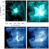 |
Fig. 1. a: AIA 131 Å image at 12:49:09 UT. The white dashed box delineates the flare region. The arrow points to the M1.2 flare. b: closeup of the flare region. c and d: AIA 335 Å images at 12:49:15 UT and 13:37:27 UT. The arrows point to the short main flaring loops and long late-phase loops. The whole evolution of the event observed in 131 Å and 335 Å is shown in a movie (flare.mp4) that is available online. |
In Fig. 2, SXR light curves in 0.5−4.0 Å and 1−8 Å are plotted with cyan and magenta lines in panel a. The SXR fluxes increase rapidly from ∼12:39 UT to the peak at 12:49:19 UT, before declining gradually to ∼14:30 UT. Hence, the lifetime of the flare reaches ∼110 min. The time derivative of the 1−8 Å flux during 12:30−13:00 UT is plotted with a black line in Fig. 2b. The HXR light curve at 12−25 keV from RHESSI observation is superposed with an orange line in Fig. 2b. Two peaks at ∼12:42:30 UT and ∼12:47:30 UT signify the two-stage energy release (see also Fig. 5f of Dai et al. 2018). The 131 Å and 335 Å intensities within the white dashed box of Fig. 1b are accumulated. The time evolutions of their total emissions are displayed in Figs. 2d and e (see also Fig. 1 of Dai et al. 2018). The 131 Å light curve shows a good correlation with the 1−8 Å light curve. The peak time of EUV late phase in 335 Å is ∼13:37:30 UT, which has a delay of ∼48 min relative to the SXR peak time. In the following, we focus on different energy contents of the flare.
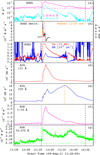 |
Fig. 2. a: SXR light curves of the flare in 0.5−4 Å and 1−8 Å. The magenta dashed line represents the background intensity. b: time derivative of the flux in 1−8 Å (black line) and HXR light curve at 12−25 keV (orange line). The red dashed lines denote the peak times of two-stage energy release. c: time evolution of the flare temperature (Te) and the emission measure (EM) derived from GOES observations. d and e: time evolution of the integral intensity of the flare in 131 Å and 335 Å. The orange dashed line denotes the peak time of EUV late phase. f and g: light curves of the flare in 1−70 and 70−370 Å. The magenta and green dashed lines represent the background intensities, respectively. |
3.2. Radiated energy
First, we calculate the radiated energy in GOES 1−8 Å. We note that the GOES XRS fluxes have been corrected by a factor of ∼1.5 (Woods et al. 2017). In Fig. 2a, the flux that comes well before the flare impulsive phase is considered as the background radiation (magenta dashed line). The background-subtracted light curve (f1−8) is plotted in Fig. 3a. The radiated energy is calculated by integrating f1−8 during 12:39−14:30 UT after multiplying a factor of c0 = 107 × 2πd2 = 1.406 × 1030 m2, where d = 1.496 × 10¹¹ m represents the average distance between the Sun and Earth (Zhang et al. 2019). The radiated energy in 1−8 Å is estimated to be ∼3.1 × 1028 erg and is listed in the first column of Table 2.
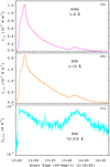 |
Fig. 3. Background-subtracted light curves of the flare in 1−8 Å, 1−70 Å, and 70−370 Å. |
Energy components (in units of 1030 erg) for the M1.2 flare.
Secondly, we calculate the radiated energy in EVE 1−70 Å. The 1−70 Å light curve of the flare is plotted in Fig. 2f. As in 1−8 Å, the flux well before the flare impulsive phase is considered as the background radiation (magenta dashed line). The background-subtracted light curve (f1−70) is plotted in Fig. 3b. The radiated energy is calculated by integrating f1−70 during 12:39−14:30 UT after multiplying c0. The radiated energy in 1−70 Å is estimated to be ∼5.4 × 1030 erg, which is ∼180 times larger than that in 1−8 Å.
Finally, we calculate the radiated energy in EVE 70−370 Å. The 70−370 Å light curve of the flare is plotted in Fig. 2g. Likewise, the flux well before the flare impulsive phase is considered as the background radiation (green dashed line). The background-subtracted light curve (f70−370) is plotted in Fig. 3c. The radiated energy is calculated by integrating f70−370 during 12:39−14:30 UT after multiplying c0. The calculated radiated energy (4.7 × 1029 erg) in 70−370 Å is one order of magnitude lower than the radiative output in 1−70 Å. Hence, the total radiated energy in 1−370 Å reaches ∼5.9 × 1030 erg.
3.3. Radiative loss from the SXR-emitting plasma
As described in Feng et al. (2013), the total optically thin radiative loss from the SXR-emitting plasma is calculated based on EM and Te derived from GOES observations, which are drawn with blue and red lines in Fig. 2c.
 (1)
(1)
where Λ(Te) denotes the radiative loss function (Cox & Tucker 1969), which is shown in Fig. 8 of Zhang et al. (2019). The start and end times for the integral are set to be 12:39 UT and 14:00 UT, since the signals after 14:00 UT are chaotic and unconvincing. The value of Trad is estimated to be ∼1.1 × 1030 erg and is listed in the sixth column of Table 2. Trad is ∼36 times larger than the radiation in 1−8 Å, which is in line with previous results for confined flares (Zhang et al. 2019; Cai et al. 2021).
3.4. Peak thermal energy of the SXR-emitting plasma
The thermal energy of the SXR-emitting plasma is calculated as:
 (2)
(2)
where  is the electron number density, kB = 1.38 × 10⁻¹⁶ erg K−1 is the Boltzmann constant, V is the total volume of the hot plasma, and f ≈ 1 represents the volumetric filling factor (Stoiser et al. 2007; Emslie et al. 2012).
Despite the large size of flare region in Fig. 1b, we note that a significant proportion of the flare region is not filled with hot plasma in 3D, which is indicated in Fig. 7c of Dai et al. (2018). Therefore, the volume of the SXR-emitting plasma is given as the total volume of magnetic flux tubes rooted in the three flare ribbons (R1, R2, and R3) in the chromosphere. In Fig. 4, the left panel shows the AIA 1600 Å image at 12:42:41 UT. Two parallel ribbons (R1 and R2) and one short ribbon (R3) very close to R2 are obviously demonstrated. Three representative points (green lines) on R1 are selected. In panels b–d, the intensity distributions across the ribbon are displayed with blue lines and the results of Gaussian fitting are displayed with red lines. The full width at half maximum (FWHM) of the Gauss function lies in the range from 1 5 to 2″. The mean value (1
 8) is taken to be the width of flare ribbons. The area of R1 can be expressed as AR1 = lR1 × w, where lR1 = 115″ and
  denote the length and width of R1. Likewise, the area of R2 is expressed as AR2 = lR2 × w, where lR2 = 130″ and
  denote the length and width of R2.
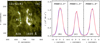 |
Fig. 4. a: AIA 1600 Å image at 12:42:41 UT. R1, R2, and R3 signify the three flare ribbons. Three representative points (green lines) are selected. b–d: intensity distributions across the ribbon (blue lines) and results of Gaussian fitting (red lines). The values of FWHM are labeled. |
As mentioned above, the post-flare loops are composed of two groups: the short main flaring loops and long late-phase loops. The former is rooted in R2 and R3, and the latter is rooted in R1 and R2. In Fig. 5, we draw a simplified schematic cartoon to illustrate the magnetic connections from top view and side view. Both the main flaring loops (magenta lines) and late-phase loops (cyan lines) are assumed to have a semi-circular shape. The footpoint area of main flaring loops is taken to be equal to AR2 and the footpoint area of late-phase loops is taken to be equal to AR1. The calculated values of AR1 and AR2 are listed in the second column of Table 3. The total length (2L) of the main flaring loops and late-phase loops are taken to be 10−25 Mm and ∼110 Mm based on the stereoscopic measurement (Dai et al. 2018), which are listed in the third column of Table 3. Accordingly, the volume of main flaring loops is calculated to be 2L × AR2 = (1.2−3.0) × 1027 cm3. The volume of late-phase loops is calculated to be 2L × AR1 = 1.2 × 1028 cm3. The total volume of post-flare loops consisting of the main-flaring loops and late-phase loops has a range (1.3−1.5) × 1028 cm3. According to Eq. (2), the peak thermal energy of the flare is calculated to be (1.7−1.8) × 1030 erg and is listed in the sixth column of Table 2. The heating requirement of hot plasma, including the peak thermal energy and radiative loss, is (2.8−2.9) × 1030 erg.
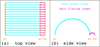 |
Fig. 5. Schematic cartoon showing the top view (a) and side view (b) of the main flaring loops (magenta lines) and late-phase loops (cyan lines), respectively. |
Physical parameters of the main flaring loops and late-phase loops, including the footpoint area, total loop length, volume, and energy input.
3.5. Energy input in main flaring loops and EUV late-phase loops
Using the EBTEL code and observed parameters, Dai et al. (2018) performed a zero-dimensional (0D) numerical simulation to study the thermodynamic evolution of a typical EUV late-phase loop. The imposed heating rate as a function of time is expressed as:
 (3)
(3)
where H0 denotes the amplitude of heating rate and τ = 23 s denotes the Gaussian heating duration. The best-fit value of H0 (1.1 erg cm−3 s−1) is larger than previously reported values (Sun et al. 2013; Li et al. 2014; Zhou et al. 2019). The energy input in the flare loops is expressed as Ein = V × ∫H(t)dt erg. Assuming that the heating durations and amplitudes of heating rate are the same for each of the late-phase loops, the energy input in late-phase loops reaches ∼7.7 × 1029 erg. For the main flaring loops (as mentioned in Sect. 3.1), both of the two-stage energy release processes contribute to the heating. Hence, the heating duration of the main flaring loops is double compared with the late-phase loops. Assuming that the amplitude of heating rate is equal to H0, the energy input in the main flaring loops is estimated to be (1.5−3.8) × 1029 erg. Based on the EBTEL simulation, the energy input in the post-flare loops amounts to (9.2−11.5) × 1029 erg.
3.6. Nonthermal energy in flare-accelerated electrons
Under the thick-target assumption (Fletcher et al. 2013), HXR emissions at the footpoints are produced by collisional bremsstrahlung during the passage of flare-accelerated nonthermal electrons through a dense target, where the electrons are stopped by Coulomb collisions and lose energy in the chromosphere. The localized plasma can be heated up to ∼10 MK accompanied by chromospheric evaporation and condensation (Tian et al. 2014; Li et al. 2015; Zhang et al. 2016a,b; Zhou et al. 2020). The distribution of injected nonthermal electrons above a low-energy cutoff (Ec) is assumed to be in the form of single power law with a spectral index of δ,  , where A0 is a normalized parameter of the total electron flux (in units of 1035 electrons s−1). In Fig. 6, three characteristic HXR spectra made from detector 9 of RHESSI during the first stage of energy release are displayed. In each panel, the fitted thermal component is drawn with a red line, while the nonthermal component is drawn with a blue line. It is obvious that the isothermal temperatures from RHESSI are close to those derived from GOES.
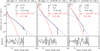 |
Fig. 6. Three characteristic HXR spectra with an integration time of 20 s (black lines) and the fitted thermal (red lines) and nonthermal (blue lines) components. Te and EM of the thermal component are labeled. The low-energy cutoff (Ec), spectral index (δ) of nonthermal electrons, and |

The delivered energy by nonthermal electrons above Ec is calculated by integrating the injected power during 12:40−12:46 UT,
 (4)
(4)
where Ant is the electron injection area, EH is set to be 30 MeV (Warmuth & Mann 2016a). The nonthermal energy in flare-accelerated electrons during the first stage is estimated to be ∼1.74 × 1030 erg.
Considering that the HXR observation from RHESSI was unavailable during the second stage of energy release around 12:47:30 UT, it is impossible to calculate the nonthermal energy of electrons from RHESSI during the second stage. In Fig. 2b, the second peak of GOES derivative accounts for ∼1/4 of the first peak, implying that energy input during the second stage accounts for ∼1/4 of the first stage. In this way, the nonthermal energy in the flare-accelerated electrons during the second stage is crudely estimated to be 0.44 × 1030 erg. Therefore, the total nonthermal energy in electrons lies in the range of (1.7−2.2) × 1030 erg. It is clear that the nonthermal energy input by flare-accelerated electrons is slightly larger than the peak thermal energy and is adequate to provide the energy input of main flaring loops and late-phase loops, which is consistent with the collisional thick-target model.
3.7. Magnetic free energy
As mentioned in Sect. 1, the energies in flares and CMEs come from the pre-stored free energy in the non-potential magnetic fields prior to eruption (Aschwanden et al. 2014). The magnetic energy is defined as  . The free energy of the non-potential field is defined as
  , where
  and
and  signify the magnetic energies in the non-potential and potential field (Guo et al. 2008). Figure 7 shows the HMI LOS magnetogram at 12:20:07 UT, featuring a strong positive polarity (P2) surrounded by negative polarities (N1). A weak and disperse positive polarity (P1) is located to the east of N1. The 3D magnetic topology of AR 11283 at 12:20 UT is obtained by using the NLFFF extrapolation (see Fig. 7 of Dai et al. 2018). The magnetic free energy before the flare is calculated to be 9.1 × 1031 erg, which is on the same order of magnitude as the X3.4 flare on 2006 December 13 (Guo et al. 2008). It is clear that the magnetic free energy is ≥40 times higher than the nonthermal energy in electrons. Therefore, the free energy is sufficient to account for the plasma heating, the acceleration of nonthermal particles, and radiations.
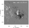 |
Fig. 7. HMI LOS magnetogram at 12:20:07 UT. P1 and P2 denote the positive polarities. N1 denotes the negative polarities surrounding P2. |
4. Discussion
Thus far, complete investigations of energy partition in eruptive flares are abundant (Emslie et al. 2004, 2005, 2012; Warmuth & Mann 2016a,b; Aschwanden et al. 2017). However, the energy partition in confined flares is rarely explored. Zhang et al. (2019) calculated the energy components of two M1.1 confined flares in AR 12434, finding that the two flares bear some similarity in morphology, evolution, and energy partition. In addition, the nonthermal energy in electrons is sufficient to supply the total heating requirement. In this paper, the M1.2 flare in AR 11283 has a much longer lifetime (∼110 min) owing to the extremely large EUV late phase. The radiated energy in 1−70 Å and total radiative loss are four to six times larger than the M1.1 CRFs. The peak thermal energy is comparable with that of CRFs. The nonthermal energy in electrons account for ∼50% that of CRFs.
The separate radiated energies in the main phase and late phase may change from case to case. For the M1.0 confined flare on 2010 November 5, the radiation in EVE 6−37 nm in the late phase is significantly larger than that in the main phase (Liu et al. 2015). On the contrary, for the X1.3 eruptive flare on 2014 April 25, the radiation in the main phase is twelve times larger than that in the late phase (Zhou et al. 2019). For the M1.2 flare considered in our study, there is no distinct demarcation point between the main phase and late phase.
Motorina et al. (2020) studied a flare as a result of loop-loop interaction on 2013 November 5. One loop is tenuous and hot, while the other is dense and cool. The released magnetic energy is converted to the nonthermal energy of accelerated electrons with a high efficiency and further converted to the thermal energy of the plasma. Meanwhile, the energy is deposited equally in the two flaring loops. In our study, the main flaring loops are short (10−25 Mm) and the late-phase loops are long (∼110 Mm). The ratio of energy input in the main flaring loops to that in late-phase loops is ≤1/2 (see Table 3).
It should be emphasized that our calculation of energy components has its limitations. The estimation of volume of the SXR-emitting plasma is based on a simplified schematic cartoon considering that the true morphology of the evolving post-flare loops is unknown. The calculation of nonthermal energy in flare-accelerated electrons carries a large uncertainty since there was no HXR observation during the second stage of energy release. In addition, the nonthermal energy in flare-accelerated ions is not considered. The energy transported to the upper chromosphere by Alfvén wave is not easy to quantify (Fletcher & Hudson 2008; Reep & Russell 2016). Subsequent case studies are needed to get a better understanding of the complete energy partition in confined flares.
5. Summary
In this paper, we reanalyze the M1.2 confined flare with a large EUV late phase observed by SDO, GOES, and RHESSI on 2011 September 9, with a focus on its energy partition. We calculate various energy components of the flare, including the magnetic free energy, peak thermal energy, nonthermal energy of flare-accelerated electrons, total radiative loss of hot plasma, and radiative outputs in 1−8 Å, 1−70 Å, and 70−370 Å. The main results are summarized below:
-
The radiation (∼5.4 × 1030 erg) in 1−70 Å is nearly eleven times larger than the radiation in 70−370 Å, and is nearly 180 times larger than the radiation in 1−8 Å.
-
The peak thermal energy of the post-flare loops is estimated to be (1.7−1.8) × 1030 erg based on a simplified schematic cartoon. Based on previous results of EBTEL simulation, the energy inputs in the main flaring loops and late-phase loops are (1.5−3.8) × 1029 erg and 7.7 × 1029 erg, respectively.
-
The nonthermal energy ((1.7−2.2) × 1030 erg) of the flare-accelerated electrons is comparable to the peak thermal energy and is sufficient to provide the energy input of the main flaring loops and late-phase loops. The magnetic free energy (9.1 × 1031 erg) before flare is large enough to provide the heating requirement and radiation, corroborating the magnetic origin of confined flares.
Movie
Movie 1 associated with Fig. 1 (flare) Access Supplementary Material
Acknowledgments
The authors thank the referee for valuable and constructive suggestions. SDO is a mission of NASA’s Living With a Star Program. AIA and HMI data are courtesy of the NASA/SDO science teams. This work is funded by the B-type Strategic Priority Program of the Chinese Academy of Sciences, Grant No. XDB41000000, NSFC grants (No. 11773079, 11790302, 11373023, 11673048), CAS Key Laboratory of Solar Activity, National Astronomical Observatories (KLSA202006), the Youth Innovation Promotion Association CAS, the Strategic Priority Research Program on Space Science, CAS (XDA15052200, XDA15320301), and the Science and Technology Development Fund of Macau (275/2017/A). Y.D. is also sponsored by the Open Research Project of National Center for Space Weather, China Meteorological Administration.
References
- Amari, T., Canou, A., Aly, J.-J., et al. 2018, Nature, 554, 211 [NASA ADS] [CrossRef] [Google Scholar]
- Aschwanden, M. J., Xu, Y., & Jing, J. 2014, ApJ, 797, 50 [NASA ADS] [CrossRef] [Google Scholar]
- Aschwanden, M. J., Boerner, P., Ryan, D., et al. 2015, ApJ, 802, 53 [NASA ADS] [CrossRef] [Google Scholar]
- Aschwanden, M. J., Caspi, A., Cohen, C. M. S., et al. 2017, ApJ, 836, 17 [NASA ADS] [CrossRef] [Google Scholar]
- Baumgartner, C., Thalmann, J. K., & Veronig, A. M. 2018, ApJ, 853, 105 [Google Scholar]
- Brown, J. C. 1971, Sol. Phys., 18, 489 [NASA ADS] [CrossRef] [Google Scholar]
- Cai, Z. M., Zhang, Q. M., Ning, Z. J., et al. 2021, Sol. Phys., 296, 61 [Google Scholar]
- Cargill, P. J. 1994, ApJ, 422, 381 [Google Scholar]
- Cargill, P. J., Bradshaw, S. J., & Klimchuk, J. A. 2012a, ApJ, 752, 161 [NASA ADS] [CrossRef] [Google Scholar]
- Cargill, P. J., Bradshaw, S. J., & Klimchuk, J. A. 2012b, ApJ, 758, 5 [NASA ADS] [CrossRef] [Google Scholar]
- Chamberlin, P. C., Milligan, R. O., & Woods, T. N. 2012, Sol. Phys., 279, 23 [NASA ADS] [CrossRef] [Google Scholar]
- Chen, J., Liu, R., Liu, K., et al. 2020, ApJ, 890, 158 [Google Scholar]
- Cox, D. P., & Tucker, W. H. 1969, ApJ, 157, 1157 [NASA ADS] [CrossRef] [Google Scholar]
- Dai, Y., & Ding, M. 2018, ApJ, 857, 99 [Google Scholar]
- Dai, Y., Ding, M. D., & Guo, Y. 2013, ApJ, 773, L21 [NASA ADS] [CrossRef] [Google Scholar]
- Dai, Y., Ding, M., Zong, W., et al. 2018, ApJ, 863, 124 [CrossRef] [Google Scholar]
- Demoulin, P., Henoux, J. C., Priest, E. R., & Mandrini, C. H. 1996, A&A, 308, 643 [NASA ADS] [Google Scholar]
- Emslie, A. G., Kucharek, H., Dennis, B. R., et al. 2004, J. Geophys. Res.: Space Phys., 109, A10104 [Google Scholar]
- Emslie, A. G., Dennis, B. R., Holman, G. D., et al. 2005, J. Geophys. Res.: Space Phys., 110, A11103 [Google Scholar]
- Emslie, A. G., Dennis, B. R., Shih, A. Y., et al. 2012, ApJ, 759, 71 [NASA ADS] [CrossRef] [Google Scholar]
- Feng, L., Wiegelmann, T., Su, Y., et al. 2013, ApJ, 765, 37 [NASA ADS] [CrossRef] [Google Scholar]
- Fletcher, L., & Hudson, H. S. 2008, ApJ, 675, 1645 [NASA ADS] [CrossRef] [Google Scholar]
- Fletcher, L., Dennis, B. R., Hudson, H. S., et al. 2011, Space Sci. Rev., 159, 19 [NASA ADS] [CrossRef] [Google Scholar]
- Fletcher, L., Hannah, I. G., Hudson, H. S., et al. 2013, ApJ, 771, 104 [NASA ADS] [CrossRef] [Google Scholar]
- Forbes, T. G., Linker, J. A., Chen, J., et al. 2006, Space Sci. Rev., 123, 251 [NASA ADS] [CrossRef] [Google Scholar]
- Guo, Y., Ding, M. D., Wiegelmann, T., et al. 2008, ApJ, 679, 1629 [NASA ADS] [CrossRef] [Google Scholar]
- Hannah, I. G., & Kontar, E. P. 2013, A&A, 553, A10 [NASA ADS] [CrossRef] [EDP Sciences] [Google Scholar]
- Inglis, A. R., & Christe, S. 2014, ApJ, 789, 116 [CrossRef] [Google Scholar]
- Ji, H., Wang, H., Schmahl, E. J., et al. 2003, ApJ, 595, L135 [NASA ADS] [CrossRef] [Google Scholar]
- Jiang, C., Feng, X., Wu, S. T., et al. 2013, ApJ, 771, L30 [NASA ADS] [CrossRef] [Google Scholar]
- Jing, J., Chen, P. F., Wiegelmann, T., et al. 2009, ApJ, 696, 84 [NASA ADS] [CrossRef] [Google Scholar]
- Klimchuk, J. A., Patsourakos, S., & Cargill, P. J. 2008, ApJ, 682, 1351 [Google Scholar]
- Kuhar, M., Krucker, S., Hannah, I. G., et al. 2017, ApJ, 835, 6 [Google Scholar]
- Lemen, J. R., Title, A. M., Akin, D. J., et al. 2012, Sol. Phys., 275, 17 [Google Scholar]
- Li, Y., Ding, M. D., Guo, Y., et al. 2014, ApJ, 793, 85 [NASA ADS] [CrossRef] [Google Scholar]
- Li, D., Ning, Z. J., & Zhang, Q. M. 2015, ApJ, 813, 59 [NASA ADS] [CrossRef] [Google Scholar]
- Lin, R. P., Dennis, B. R., Hurford, G. J., et al. 2002, Sol. Phys., 210, 3 [Google Scholar]
- Liu, K., Zhang, J., Wang, Y., et al. 2013, ApJ, 768, 150 [NASA ADS] [CrossRef] [Google Scholar]
- Liu, K., Wang, Y., Zhang, J., et al. 2015, ApJ, 802, 35 [CrossRef] [Google Scholar]
- Masson, S., Pariat, É., Valori, G., et al. 2017, A&A, 604, A76 [EDP Sciences] [Google Scholar]
- Myers, C. E., Yamada, M., Ji, H., et al. 2015, Nature, 528, 526 [NASA ADS] [CrossRef] [Google Scholar]
- Milligan, R. O., Kerr, G. S., Dennis, B. R., et al. 2014, ApJ, 793, 70 [NASA ADS] [CrossRef] [Google Scholar]
- Moore, R. L., Sterling, A. C., Hudson, H. S., et al. 2001, ApJ, 552, 833 [Google Scholar]
- Motorina, G. G., Fleishman, G. D., & Kontar, E. P. 2020, ApJ, 890, 75 [Google Scholar]
- Patsourakos, S., Vourlidas, A., Török, T., et al. 2020, Space Sci. Rev., 216, 131 [Google Scholar]
- Pesnell, W. D., Thompson, B. J., & Chamberlin, P. C. 2012, Sol. Phys., 275, 3 [Google Scholar]
- Prasad, A., Dissauer, K., Hu, Q., et al. 2020, ApJ, 903, 129 [Google Scholar]
- Priest, E. R., & Forbes, T. G. 2002, A&ARv, 10, 313 [NASA ADS] [CrossRef] [Google Scholar]
- Reames, D. V. 2015, Space Sci. Rev., 194, 303 [Google Scholar]
- Reep, J. W., & Russell, A. J. B. 2016, ApJ, 818, L20 [NASA ADS] [CrossRef] [Google Scholar]
- Reeves, K. K., Linker, J. A., Mikić, Z., et al. 2010, ApJ, 721, 1547 [NASA ADS] [CrossRef] [Google Scholar]
- Saint-Hilaire, P., & Benz, A. O. 2002, Sol. Phys., 210, 287 [NASA ADS] [CrossRef] [Google Scholar]
- Scherrer, P. H., Schou, J., Bush, R. I., et al. 2012, Sol. Phys., 275, 207 [Google Scholar]
- Schrijver, C. J., DeRosa, M. L., Metcalf, T., et al. 2008, ApJ, 675, 1637 [Google Scholar]
- Song, H. Q., Zhang, J., Cheng, X., et al. 2014, ApJ, 784, 48 [NASA ADS] [CrossRef] [Google Scholar]
- Stoiser, S., Veronig, A. M., Aurass, H., et al. 2007, Sol. Phys., 246, 339 [NASA ADS] [CrossRef] [Google Scholar]
- Sun, X., Hoeksema, J. T., Liu, Y., et al. 2013, ApJ, 778, 139 [NASA ADS] [CrossRef] [Google Scholar]
- Sun, X., Bobra, M. G., Hoeksema, J. T., et al. 2015, ApJ, 804, L28 [Google Scholar]
- Thalmann, J. K., Su, Y., Temmer, M., et al. 2015, ApJ, 801, L23 [NASA ADS] [CrossRef] [Google Scholar]
- Tian, H., Li, G., Reeves, K. K., et al. 2014, ApJ, 797, L14 [NASA ADS] [CrossRef] [Google Scholar]
- Wang, Y., & Zhang, J. 2007, ApJ, 665, 1428 [NASA ADS] [CrossRef] [Google Scholar]
- Wang, Y., Ji, H., Warmuth, A., et al. 2020, ApJ, 905, 126 [Google Scholar]
- Warmuth, A., & Mann, G. 2016a, A&A, 588, A115 [NASA ADS] [CrossRef] [EDP Sciences] [Google Scholar]
- Warmuth, A., & Mann, G. 2016b, A&A, 588, A116 [NASA ADS] [CrossRef] [EDP Sciences] [Google Scholar]
- Warmuth, A., & Mann, G. 2020, A&A, 644, A172 [EDP Sciences] [Google Scholar]
- White, S. M., Thomas, R. J., & Schwartz, R. A. 2005, Sol. Phys., 227, 231 [NASA ADS] [CrossRef] [Google Scholar]
- Woods, T. N., Hock, R., Eparvier, F., et al. 2011, ApJ, 739, 59 [Google Scholar]
- Woods, T. N., Eparvier, F. G., Hock, R., et al. 2012, Sol. Phys., 275, 115 [Google Scholar]
- Woods, T. N., Caspi, A., Chamberlin, P. C., et al. 2017, ApJ, 835, 122 [Google Scholar]
- Xia, F., Su, Y., Wang, W., et al. 2021, ApJ, 908, 111 [Google Scholar]
- Yan, X., Xue, Z., Cheng, X., et al. 2020, ApJ, 889, 106 [NASA ADS] [CrossRef] [Google Scholar]
- Zhang, J., Dere, K. P., Howard, R. A., et al. 2001, ApJ, 559, 452 [Google Scholar]
- Zhang, Q. M., Ning, Z. J., Guo, Y., et al. 2015, ApJ, 805, 4 [NASA ADS] [CrossRef] [Google Scholar]
- Zhang, Q. M., Li, D., Ning, Z. J., et al. 2016a, ApJ, 827, 27 [NASA ADS] [CrossRef] [Google Scholar]
- Zhang, Q. M., Li, D., & Ning, Z. J. 2016b, ApJ, 832, 65 [NASA ADS] [CrossRef] [Google Scholar]
- Zhang, Q. M., Cheng, J. X., Feng, L., et al. 2019, ApJ, 883, 124 [Google Scholar]
- Zhou, Z., Cheng, X., Liu, L., et al. 2019, ApJ, 878, 46 [Google Scholar]
- Zhou, Y.-A., Li, Y., Ding, M. D., et al. 2020, ApJ, 904, 95 [Google Scholar]
All Tables
Physical parameters of the main flaring loops and late-phase loops, including the footpoint area, total loop length, volume, and energy input.
All Figures
|
Fig. 1. a: AIA 131 Å image at 12:49:09 UT. The white dashed box delineates the flare region. The arrow points to the M1.2 flare. b: closeup of the flare region. c and d: AIA 335 Å images at 12:49:15 UT and 13:37:27 UT. The arrows point to the short main flaring loops and long late-phase loops. The whole evolution of the event observed in 131 Å and 335 Å is shown in a movie (flare.mp4) that is available online. |
| In the text | |
|
Fig. 2. a: SXR light curves of the flare in 0.5−4 Å and 1−8 Å. The magenta dashed line represents the background intensity. b: time derivative of the flux in 1−8 Å (black line) and HXR light curve at 12−25 keV (orange line). The red dashed lines denote the peak times of two-stage energy release. c: time evolution of the flare temperature (Te) and the emission measure (EM) derived from GOES observations. d and e: time evolution of the integral intensity of the flare in 131 Å and 335 Å. The orange dashed line denotes the peak time of EUV late phase. f and g: light curves of the flare in 1−70 and 70−370 Å. The magenta and green dashed lines represent the background intensities, respectively. |
| In the text | |
|
Fig. 3. Background-subtracted light curves of the flare in 1−8 Å, 1−70 Å, and 70−370 Å. |
| In the text | |
|
Fig. 4. a: AIA 1600 Å image at 12:42:41 UT. R1, R2, and R3 signify the three flare ribbons. Three representative points (green lines) are selected. b–d: intensity distributions across the ribbon (blue lines) and results of Gaussian fitting (red lines). The values of FWHM are labeled. |
| In the text | |
|
Fig. 5. Schematic cartoon showing the top view (a) and side view (b) of the main flaring loops (magenta lines) and late-phase loops (cyan lines), respectively. |
| In the text | |
|
Fig. 6. Three characteristic HXR spectra with an integration time of 20 s (black lines) and the fitted thermal (red lines) and nonthermal (blue lines) components. Te and EM of the thermal component are labeled. The low-energy cutoff (Ec), spectral index (δ) of nonthermal electrons, and |
| In the text | |
|
Fig. 7. HMI LOS magnetogram at 12:20:07 UT. P1 and P2 denote the positive polarities. N1 denotes the negative polarities surrounding P2. |
| In the text | |
Current usage metrics show cumulative count of Article Views (full-text article views including HTML views, PDF and ePub downloads, according to the available data) and Abstracts Views on Vision4Press platform.
Data correspond to usage on the plateform after 2015. The current usage metrics is available 48-96 hours after online publication and is updated daily on week days.
Initial download of the metrics may take a while.