| Issue |
A&A
Volume 649, May 2021
|
|
|---|---|---|
| Article Number | A131 | |
| Number of page(s) | 12 | |
| Section | Planets and planetary systems | |
| DOI | https://doi.org/10.1051/0004-6361/202140359 | |
| Published online | 27 May 2021 | |
A transmission spectrum of the planet candidate WD 1856+534 b and a lower limit to its mass★
1
Instituto de Astrofísica de Canarias,
38205
La Laguna,
Tenerife,
Spain
e-mail: This email address is being protected from spambots. You need JavaScript enabled to view it.
2
Departamento de Astrofísica, Universidad de La Laguna,
38206
La Laguna,
Tenerife,
Spain
3
Gran Telescopio Canarias (GTC),
38712,
Breña Baja,
La Palma,
Spain
4
Department of Physics, The University of Warwick,
Coventry
CV4 7AL,
UK
Received:
15
January
2021
Accepted:
29
March
2021
Abstract
The cool white dwarf WD 1856+534 was found to be transited by a Jupiter-sized object with a mass at or below 14 MJup. We used the GTC telescope to obtain and analyse the photometry and low-resolution spectroscopy of six transits of WD 1856+534 b, with the intention of deriving the slope of the transmission spectrum. Such a slope, assuming a cloud-free atmosphere dominated by Rayleigh scattering of the particles in its atmosphere, could be translated into an estimation of the mass of WD 1856+534 b. However, the resultant transmission spectrum is essentially flat and therefore permits only the determination of lower mass limits of 2.4 MJup at the 2σ level, or 1.6 MJup at 3σ. These limits have implications for some of the formation scenarios proposed for the object. We elaborate on the potential effects of clouds and hazes in our estimations, based on previous studies of Jupiter and Titan. In addition, we detected an Hα absorption feature in the combined spectrum of the host white dwarf, which leads to the assignation of a DA classification and allows the derivation of an independent set of atmospheric parameters. Furthermore, the epochs of five transits were measured with sub-second precision, which demonstrates that additional objects more massive than ≈5 MJup and with periods longer than O(100) days could be detected through the light-time effect.
Key words: white dwarfs / planets and satellites: fundamental parameters / techniques: photometric / techniques: spectroscopic
Based on observations made with the Gran Telescopio Canarias (GTC), on the island of La Palma at the Spanish Observatorio del Roque de los Muchachos of the IAC, under Director’s Discretionary Time GTC2020-144.
© ESO 2021
1 Introduction
White dwarfs (WDs) are the final product of the evolution of stars with masses between one and eight solar masses. In recent decades, growing evidence has been obtained regarding the presence of planetary material around some of these objects in the form of debris disks (e.g. Farihi 2016; Rebassa-Mansergas et al. 2019) and/or metal pollution in their atmospheres (Zuckerman et al. 2003, 2010; Koester et al. 2014).
With the Kepler space telescope (Borucki et al. 2010), Vanderburg et al. (2015) found disintegrating material transiting the hot WD 1145+07. These transits exhibit varying depths and shapes as well as periodicities in the 4.5–4.9 h range (e.g. Alonso et al. 2016; Gary et al. 2017; Izquierdo et al. 2018), which is compatible with clouds transiting due to the evaporation of drifting asteroid fragments orbiting the WD (Rappaport et al. 2016). Vanderbosch et al. (2020) found another similar case, but with a much longer period of ≈107.2 days, in ZTF J013906.17+524536.89.
The existence of planets can also be inferred from the characteristics of their debris disks or from their atmospheric pollution. Among the few dozen metal-polluted WDs studied so far, Manser et al. (2019) detected a stable 123 min periodic variation in the Ca II emission lines of the WD SDSS J122859.93+104032.9; their interpretation involves a solid body with a size between 2 and 600 km at a distance of 0.73 R⊙ under the assumption of a circular orbit. Similarly, the composition of the circumstellar gaseous disk of the hot WD SDSS J091405.30+191412.2 resembles the predictions for the deeper layers of icy giant planets (Gänsicke et al. 2019). In their scenario, a giant planet orbiting at about 15 R⊙ would be undergoing evaporation of its atmosphere, which would then be accreted onto the WD.
Regarding the target of this paper, WD 1856+534, Vanderburg et al. (2020, V20 hereafter) found transits in data from the TESS mission (Ricker et al. 2015), indicating a planet candidate with a size comparable to that of Jupiter. With an orbital period of 1.4 days, its 8 min long grazing transits imply that a substantial fraction of the WD is occulted, reaching transit depths of ≈ 57%. Nearly identical transit depths observed in the Sloan g filter and the Spitzer 4.5 μm channel were used by V20 to provide an upper limit to the mass of the giant planet candidate of 14 MJup. They determined the host WD as a nearby (~25 pc) cool (Teff = 4710 ± 60 K) stellar remnant that is also a known member of a triple system, with two M dwarfs separated by 58 AU orbiting the WD at a projected distance of ≈ 1500 AU.
These companion M dwarfs have been used to explain the evolution and current orbit of the planet candidate via the Zeipel–Lidov–Kozai (ZKL) mechanism (von Zeipel 1910; Lidov 1962; Kozai 1962), something that is explored in detail in three works: Muñoz & Petrovich (2020) use the ZKL mechanism to constrain the primordial semi-major axis (during the main sequence of the host star) and mass of the companion to 2–2.5 AU and 0.7–3 MJup, respectively.Two other works obtain less constrained primordial parameters, with a distance of 10–20 AU (O’Connor et al. 2021) or 20–100 AU (with a preference for the larger values; Stephan et al. 2020) and, in both cases, without constraints on the orbiter’s mass. Lagos et al. (2021) argue that common envelope evolution is at least as plausible as the ZKL mechanism as an explanation for the formation of WD 1856+534 b, and they predict its mass to be larger than about 5 MJup. Finally, V20 also present dynamical instabilities due to planetary multiplicity as another scenario that works more efficiently for low planet masses (super-Earths to Saturn masses; Maldonado et al. 2021).
For cool WDs such as WD 1856+534, it is not surprising to find spectra that show only a continuum, without distinguishable spectral lines, since the most common H and He transitions disappear below ≈ 5000 K and ≈ 12 000 K, respectively. This is the case for the spectra shown by V20; the absence of lines also hampers the measurement of the mass of the companion through the Doppler effect.
However, an alternative method for constraining the mass of an exoplanet has been proposed (Agol 2011; de Wit & Seager 2013): by measuring the Rayleigh scattering slope in a transmission spectrum, it is possible to estimate the occulter’s atmospheric scale height, and – given the occulter’s radius and some assumptions on the mean molecular mass of the atmosphere – its mass. In the current work, we present high precision multi-band photometry and low-resolution spectroscopy that was obtained with the 10.4 m Gran Telescopio Canarias (GTC) telescope with the aim to constrain the mass of the companion using that method.
The remainder of this paper is organised as follows. In Sect. 2, we describe the observations and data reduction of the different datasets. In Sect. 3.1, we derive the atmospheric parameters of the WD with two independent datasets: using archival photometric data and using the Hα absorption line that is detected for the first time in the GTC spectra. Sections 3.2 and 3.3 describe the analysis of the broadband time series photometry and the transmission spectroscopy. These are used in Sect. 3.4 to constrain the mass of the transiting object. As a by-product, accurate transit timings of sub-second precisions were obtained; in Sect. 3.5 we refine the current ephemeris and look for deviations from linearity. Finally, in Sects. 4 and 5 we discuss the results and present our conclusions.
Log of the GTC observations.
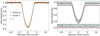 |
Fig. 1 Light curves of WD 1856+534 obtained with GTC in three different filters. In the right panel, the curves are plotted introducing vertical offsets (to observe the cadence and precision of each of the datasets) and also show the residuals of the best-fit model. The dispersions of the residuals in each colour are 0.6, 0.4, and 0.9%, respectively. |
2 Observations and data reduction
2.1 GTC photometry
We first observed WD 1856+534 during a transit event on the night of March 2, 2020 using the frame-transfer photometric mode of the GTC’s OSIRIS instrument (Cepa et al. 2000) with a Sloan i filter (see Table 1 for a list of observations and their configurations). The exposure time was 5 s, which is also the cadence of the light curve. We extracted the light curve with the HiPERCAM data reduction package (Dhillon et al. 2018)using a variable aperture and one reference star to compute the differential and normalised light curve (Fig. 1). The dispersion of the residuals at the time of transit, after subtracting the transit model described inSect. 3, is 0.4% per data point. For consistency, we also re-analysed the GTC data from October 21, 2019 presented in V20, which had been obtained with the same observing setup, except for the Sloan g filter and exposure time. Using the same reduction procedure, the dispersion of the residuals in this case is 0.6%.
Furthermore, on June 13, 2020 we obtained J-band photometry (centred at 1.25 μm) using the GTC’s EMIR instrument (Garzón et al. 2016). The observing strategy was similar to that in Alonso et al. (2008): We obtained a series of images in the “stare” mode during a predicted transit, with an exposure time of 10 sin a pre-selected region of the detector that had few cosmetic defects. To correct for the variable background emission, which might arise from changes in the thermal background or in pixel sensitivities, we obtainedsequences of images before and after the transit observation, in which the target is offset by ≈ 30′′ in a direction that avoids placing other bright objects in the region where the target was acquired during the transit. All the images were calibrated using standard procedures. The offset images from before and after the transits were averaged using sigma clipping, and the two resulting images were averaged to obtain a sky frame. This frame was subtracted from each of the images of the stare sequence. From them, we extracted the fluxes of the target and of the reference star using the same HiPERCAM data reduction package as in the visual-band images described above. After the fitting process described in Sect. 3, the dispersion of the residuals is 0.9%.
The extracted light curves in the three different bandpasses are shown in Fig. 1. The three light curves are remarkably similar, which is to be expected if the emission of the secondary component (i.e. the candidate planet) is negligible in all these bands.
2.2 GTC spectroscopy
Three more transits were observed, on May 3, 10, and 20, 2020 using the spectroscopic mode of OSIRIS, the first one with the R1000R grism and the two later ones with the R1000B grism (see Table 1). We mostly used a 2.5′′ slit and rotated the slit to include both WD 1856+534 and a slightly brighter nearby star, identified as Gaia DR2 2146576727003500032, at a distance of ≈ 1′.
The May 3, 2020 observations with the R1000R grism suffered strongly variable and poor seeing conditions; despite being analysed with the same procedures as described below, the results were not of sufficient quality, and we did not include them in any subsequent analysis. During the May 10, 2020 observations, now with the R1000B grism, the spectrum of the target was accidentally placed very close to a bad column of the detector. We repeated the observations on the night of May 20, 2020 placing the spectrum at a more favourable location of the detector. We used integration times of 75 s and a 500 kHz readout speed, resulting in a cadence of about 92 s. This provided a good signal during the transit spectra while also getting a reasonable sampling of the transit.
After the regular calibration of the spectra taken on the night of May 10, 2020, we applied a spline interpolation at each row of the detector to correct for the bad column located at one of the wings of the target spectra. For the two nights, the spectra of both the target and the comparison star were calibrated, sky-subtracted, and then extracted with STARLINK1 and PAMELA2 (Marsh 1989).
To obtain a high signal-to-noise off-transit reference spectrum of WD 1856+534, we computed an average spectrum from the 38 exposures taken out-of-transit on the night of May 20, 2020. In this average spectrum, the single and most prominent non-telluric feature is the Hα absorption line, which is detected with a depth of about 3% (Fig. 2). Given this detection, we consider WD 1856+534 to be of class DA, which is defined by the presence of Balmer lines and the simultaneous absence of other lines (McCook & Sion 1999). While the Hα absorption line is also detected in the out-of-transit spectra from the other nights, for the subsequent analysis we used only the May 20 spectrum so as to avoid potential systematics from the interpolation of the bad column or the poor weather conditions.
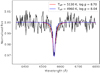 |
Fig. 2 Average out-of-transit normalised spectrum of the night of May 20, 2020 centred at the Hα absorption line. The best-fit spectroscopic model of a DA WD is overplotted as a red line, and the model that best fits the photometric data as a blue line. |
3 Data analysis
3.1 Parameters of the WD
We re-determined the atmospheric parameters of WD 1856+534 using absolute photometry from archival sources. In addition, we obtained an independent estimation of the parameters from the modelling of the Hα absorption line identified in the GTC spectra. In both cases, we used the Markov chain Monte Carlo (MCMC) EMCEE package within PYTHON (Foreman-Mackey et al. 2013) to fit a grid of model spectra to the two datasets. A synthetic grid of pure DA WDs was computed using the code in Koester (2010), spanning Teff = 4000−6000 K in steps of 250 K and log g = 7.0–9.0 in steps of 0.25 dex. We explored the whole parameter space and minimised the χ2 with 30 chains and 150 000 walkers per chain, employing uniform priors for log g and Teff. Each Teff – log g pair corresponds to a mass, MWD, radius, RWD, and cooling age, τcool, as derived from the evolutionary cooling sequences for DA WDs3 (Tremblay et al. 2011; Blouin et al. 2018; Bédard et al. 2020).
An estimation of the atmospheric parameters of WD 1856+534 using absolute photometry requires the synthetic spectra to be scaled by the solid angle of the star, 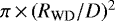 , with D being the distance to the WD. The radius is computed for each trial Teff – log g pair as explained above. The distance was derived from the Gaia early Data Release 3 (eDR3; Gaia Collaboration 2016, 2021) parallax (ϖ =40.39 ± 0.05 mas) as D = 24.76 ± 0.03 pc. To address the interstellar extinction affecting the photometric points, we reddened the grid of models by adopting E(B − V) = 0.01, which was determined from the 3D dust map produced by Stilism4 (Lallement et al. 2018). The scaled and reddened grid of models was then convolved with the bandpass of each photometric filter and compared with the observed fluxes in each filter. These fluxes had been converted from the published magnitudes using the zero points available on the Spanish Virtual Observatory (SVO) Filter Profile Service5 website. Through the MCMC fit, we obtained the Teff and log g combinationthat best matched the observation and made use of the evolutionary cooling sequences to derive the MWD, RWD, and τcool that correspond to those values. Several tests using different sets of photometric data points and distinct scaling values for the errors were performed; during these tests we were also able to replicate the results obtained by V20, who used only the Pan-STARRS1 and 2MASS photometry.However, we decided to include all available photometry in the fit and adopted the solution from the use of the Gaia eDR3, Pan-STARRS1, 2MASS, and WISE bands 1 and 2. The best fit using the published magnitude uncertainties has a reduced χ2 of ≈ 50, suggesting apoor fit or underestimated errors. We then explored different solutions by setting minimum uncertainties in the photometricmagnitudes of 0.01 and 0.05, which replaced the reported errors if they were smaller than these thresholds. They are summarised in Table 2.
We obtained an independent estimation of the effective temperature and surface gravity from the Hα absorption line. We continuum-normalised this line in both the observed and synthetic spectra by fitting a low-order polynomial to the surrounding continuum. The synthetic spectra were degraded to the resolution of the observed data (1.98 Å). The best-fit model was found for Teff = 5130 ± 55 K and log g = 8.7 ± 0.2 dex. However, we note that these are statistical uncertainties from the MCMC analysis; potentially larger systematics may arise from the use of a single spectral line in the derivation of these parameters.
For the remainder of the paper, we adopt the values from the best-fit model to the photometric data, setting a minimum uncertainty of 0.05 mag, which corresponds to the rightmost column in Table 2. Figure 2 shows the best-fit models to the spectroscopic and photometric data. We can see that, using our adopted values (blue line), the model is in reasonable agreement with the observed Hα absorption line, and it is also within the uncertainties of the values reported in V20 using pure hydrogen models (Teff = 4785 ± 60 K and log g = 7.93 ± 0.03 dex).
Derived parameters of WD 1856+534 from the photometry (Pan-STARRS1, 2MASS, WISE bands 1 and 2, and Gaia eDR3 blue and red bands), using different thresholds (Errmin) for the minimum uncertainties in the input magnitudes.
3.2 Fit of the broadband transits
We used the mass and radius of WD 1856+534 derived above as normal priors to the fit of the three transits observed in broadband photometry. To perform this fit and to obtain the posterior parameter distributions, we used the EXOPLANET package (Foreman-Mackey et al. 2020). The other parameters of the fit were: the transit epoch, Tc; the mean baseline flux, fout; the two coefficients, ub and uc, of a quadratic limb darkening law, with the sampling proposed by Kipping (2013); the radius of the secondary, Rp ; and the impact parameter, b. The finite integration times were taken into account with a factor of 5 oversampling on the fitted models. After fitting the maximum a posteriori parameters, we sampled the posteriors using the NUTS (No U-Turns Step) method (Hoffman & Gelman 2014) implementation of the PYTHON PYMC3 package6. We ran two chains with 4000 steps for tuning and 5000 draws for a final chain length of 10 000 for each of the parameters. We assessed the convergence of the chains with the Gelman & Rubin (1992) test, which was below 1.002 for each parameter. All three transits were analysed independently using the same procedure. In Table 3, we provide the mean and standard deviations of the derived parameters, and in Fig. 1 we show the best-fit models. We note that the input impact parameter, b, is much larger than 1 since this parameter is defined relative to the (small) radius of the WD. In the appendix we provide the corner plots of the posteriors to check for the correlations between the different parameters.
3.3 Transmission spectroscopy
For the study of a potential dependence of the secondary’s radius on wavelength, we make some assumptions: Regardless of the “real” size (RWD) and mass (MWD) of the host, we assume that these values are identical at every wavelength, and we fixed them to 0.0123 R⊙ and 0.606 M⊙, respectively (Sect. 3.1). A second assumption is that the impact parameter, b, is also independent of the wavelength, and we fixed it to 8.5. Selecting different values for these quantities (within the ranges given in Tables 2 and 3) has an effect on the slope of the transmission spectrum that lies within the slope’s uncertainty. Finally, the two quadratic limb darkening coefficients at each wavelength bin were fixed to results of a spline fit to the coefficients of a DA WD with Teff= 5000 K and log g = 8.0 dex, values provided by Gianninas et al. (2013).
We divided the spectra of the target into bins of different sizes, as shown in Fig. 3. These bins were selected to avoid the wavelengths affected by telluric absorptions and to be narrower when the captured signal was higher. Some fine-tuning of the number of bins between two strong telluric absorptions was performed with the aim of completely including the Hα and Na I lines inside single bins. We constructed a light curve for each wavelength bin by summing the flux of the target, summing the flux of the comparison star, dividing both, and normalising to the average out-of-transit flux.
At each wavelength bin, we fitted for the radius of the secondary, Rp, the mean out-of-transit flux, and a slope to account for potential systematic trends in the data. The rest of the parameters were held fixed, as described above. The sampling of the posterior distributions was done using the same formalism as in the previoussection. To include the broadband transit photometry, we also performed a fit were we only kept Rp, Tc, and the mean and slope of the out-of-transit flux as free parameters, while fixing b, the mass and radius of the WD, and the limb darkening coefficients.
The May 20, 2020 transmission spectrum (Fig. 4) does not show evidence of any spectral features that are dependent on the atmospheric scale height. Moreover, the spectrum is essentially flat, which is in agreement with the three data points corresponding to the transits observed in broadband filters. This is an indication of either a low atmospheric scale height of the secondary – which implies that it is a relatively massive body – or a masking of its spectral features due to having a thick cloud deck at high altitudes. In the next section, we use the broadest feature expected in giant planets, the Rayleigh scattering, to place a lower limit to the mass of the secondary. We repeated the analysis with the transit observed on May 10, 2020 in which we attempted to correct for the effects from the bad detector column in the spectra. The transmission spectrum for that night, shown in Fig. A.4, is noisier at every wavelength bin and appears to show systematically larger planetary radii that are marginally inconsistent with the photometric data points. This is indicative of residual systematic effects, and we decided not to include this spectrum in any subsequent analysis.
Derived parameters of WD 1856+534 b in the three high-cadence light curves and assuming a circular orbit.
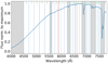 |
Fig. 3 Average out-of-transit spectrum of WD 1856+534 with the wavelength bins used to compute the transmission spectrum. The limits of the bins are represented with vertical blue lines, and the central wavelengths of each bin are indicated at the top with short vertical green lines. The definition of the bins took the locations of the telluric absorption bands into account (marked with the grey bands; these are discarded), and narrower bins were used when the flux was higher. The positions of the Na I doublet and the Hα absorption line are marked with vertical dashed red lines. |
3.4 Constraints on the mass of the secondary
The mass ofa gas giant planet can be estimated from the slope of its transmission spectrum, assuming that it is due to Rayleigh scattering in the occulter’s atmosphere: The slope is proportional to the atmospheric scale height  , where k is the Boltzmann constant, T the temperature of the atmosphere, g the surface gravity, and μ the mean molecular mass (≈2.3 for an H/He dominated atmosphere). Following de Wit & Seager (2013), the scale height for a given slope
  is then derived from:
 (1)
(1)
where the factor α describes the dependence of the cross-section of the main absorbent on wavelength; in the case of Rayleigh scattering, this is α =−4. The mass of the occulting body, Mp, is then given through:
 (2)
(2)
where G is the gravitational constant. We performed a linear fit to the transmission spectrum in Fig. 4 to obtain the slope and thus the atmospheric scale height, assuming a Rayleigh scattering regime. We included data from both the broadband imaging and the low-resolution spectra taken on May 20, 2020. For T, we took the equilibrium temperature assuming a Bond albedo of 0.35 (as in V20), a circular orbit, and isotropic re-emission of the incident flux, resulting in 165 K, which is in agreement with the values obtained by V20. The posterior distribution of the obtained scale heights is shown in Fig. 5. It shows a maximum compatible with a null slope and discards scale heights larger than 5.8, 11, and 16 km at the 1σ, 2σ, and 3σ levels, respectively. With Eq. (2) and the Rp,fix from Table 3, these heights can be translated to corresponding minimum masses of 4.4, 2.4, and 1.6 MJup.
We revised the values that would arise from relaxing the assumptions that enter into these fits. First, we explored the posterior distribution of the mass when the secondary’s estimated temperature is at the lowest reasonable level by assuming a Bond albedo of 0.6 and a RWD at the lower end (0.0118 R⊙), resulting in T = 143 K. The smaller value of RWD in this grazing configuration implies a larger inferred Rp of 1.11 RJup with a higher impact parameter to match the total duration of the transit (see the corner plots in the appendix). With these assumptions, the 1σ, 2σ, and 3σ levels of themaximum scale heights and minimum masses are 6.3, 11, and 17 km, or 4.0, 2.3, and 1.5 MJup, respectively. An exploration of the higherend value of RWD (0.0128 R⊙) implies a smaller Rp of 0.95 RJup, which, under the same assumptionsas before, results in T = 149 K and 1σ, 2σ, and 3σ levels of themaximum scale heights and minimum masses of 4.1, 9.6, and 15 km, or 4.8, 2.0, and 1.3 MJup, respectively.From these tests we can conclude that relaxing the assumptions has only minor consequences on the determined lower mass limits for the secondary companion.
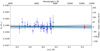 |
Fig. 4 Transmission spectrum of WD 1856+534 b. The radius of the WD is fixed to the estimated average value (0.0123 R⊙), and the impact parameter is held fixed at a given value (8.5) as both parameters are independent of the wavelength. The larger filled circles mark the radius of the secondary in the Sloan g (cyan), Sloan i (green), and EMIR J (red) filters, while dark blue dots mark the radii determined at each spectral bin defined in Fig. 3. The solid blue lines in the background are random samples of the posterior of the linear fits to measure the atmospheric scale height. We note the logarithmic scale in the x-axis. The verticalscale on the right side gives the difference in kilometres from the mean radius of the secondary. |
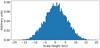 |
Fig. 5 Histogram of the scale heights obtained from the fits to the slope of the transmission spectrum shown in Fig. 4. |
Measured mid-transit epochs of WD 1856+534.
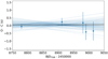 |
Fig. 6 O–C values of the mid-transit times for which a precision of less than 1 s could be achieved. The lines are random samples of the posterior of a linear fit to these values. |
3.5 Ephemeris improvement
Precise measurement of the mid-transit epochs is a widely used method to search for dynamical interactions between different planets in planetary systems (see Agol & Fabrycky 2018 for a review). An additional effect is the Rømer or light-time effect (LITE), which is due to the movement of the barycentre of a system of more than two bodies (e.g. Irwin 1959). With the transits of WD 1856+534 b being deep and short, it is possible to accurately measure the central times with a precision that is comparable to the one achieved for post-common envelope binaries (e.g. Marsh 2018). As part of the fitting process in the previous sections, the mid-transit times were measured with an accuracy of less than 1 s for all GTC observations, except for the one affected by bad weather. The epochs and corresponding errors are given in Table 4. We used these times to refine the ephemeris of V20 to:
![Mathematical equation: \begin{equation*} T_0 (\textrm{BJD}_{\textrm{TDB}}) = 2458779.375086[2] + E \,{\times}\, 1.40793913[2], \end{equation*}](/articles/aa/full_html/2021/05/aa40359-21/aa40359-21-eq6.png) (3)
(3)
where the numbers in brackets indicate the uncertainty of the last digit. The corresponding observed minus calculated (O−C) diagram is shown in Fig. 6.
4 Discussion
The observed transmission spectrum of WD 1856+534 b is consistent with being flat. This is an indication of either (i) a cloud layer at low pressure levels and high altitudes that masks any absorption or scattering feature or (ii) a low atmospheric scale height, indicating a secondary companion more massive than a few Jupiter masses.
The equilibrium temperature of WD 1856+534 b of T ≈165 ± 20 K is the second lowest known for transiting Jupiter-sized exoplanets, about 30 K warmer than the long-period planet Kepler-167e (P = 1071 day, Kipping et al. 2016)and around 50 K warmer than Jupiter. Efforts to obtain Jupiter’s transmission spectrum by observing its shadow projected on one of its moons (Montañés-Rodríguez et al. 2015; López-Puertas et al. 2018) showed that the optical part of the transmission spectrum of Jupiter is dominated by extinction from aerosols. Rayleigh scattering from the gas in Jupiter was a minor contributor to that transmission spectrum, as shown in Fig. 3 of López-Puertas et al. (2018). In the polar regions of Jupiter, both in situ probes and ground-based observations have revealed a high altitude haze layer that is best understood with fractal aggregates of monomers with an effective radius of about 0.7 μm (West & Smith 1991; Zhang et al. 2013). These hazes are thought to be similar on Titan, for which detailed near-infrared (NIR; 0.88 to 5 μm) and far-UV (0.11 to 0.19 μm) transmission spectra were obtained during solar occultations of NASA’s Cassini spacecraft (Robinson et al. 2014 and Tribbett et al. 2020, respectively). Robinson et al. (2014) analysed the NIR spectra using a simple haze extinction model with a slope of − 1.9 ± 0.2. This slope is smaller than that induced by pure Rayleigh scattering (−4). Robinson et al. (2014) explain this slope as resulting from the complexities of the scattering by haze particles when they are in an intermediate regime between the limits of Rayleigh scattering and geometrical optics. If the same type of haze is present in our transmission spectrum, and assuming a slope of − 2, this would translate into scale heights larger by a factor of about 2, and the secondary’s lower mass limits would be ≈ 2 times smaller.
Cloud decks are also frequently invoked to explain flat transmission spectra; for example, for super-Earth planets, Howe & Burrows (2012) show that cloud decks at the 10 mbar level or higher effectively suppress the characteristic slope of the Rayleigh scattering. Cloud decks on Jupiter are, however, confined to pressures of 0.5–1.2-bar or higher, whereas Jupiter’s haze layer exists at pressures of ≈ 50 mbar at low latitudes and ≈20 mbar at high latitudes (Guerlet et al. 2020). For cool exoplanets, hazes are therefore more likely to affect transmission spectra in the optical range and to ‘drown out’ the slopes from Rayleigh scattering from the gas.
The high altitude hazes at the polar region of Jupiter are thought to be created through photochemical effects induced by the precipitation of energetic particles in its auroral region (Pryor & Hord 1991), which could be more important than the effect of the incident solar UV flux. In the case of WD 1856+534 b, the incident UV flux is at the level of a few times the solar flux received at Jupiter (Fig. 7), and the grazing nature of its transits implies that the region sampled is most likely a polar one. An estimation of the probability, location, and intensity of auroras in WD 1856+534 b is beyond the scope of this paper, but it seems reasonable, from the incident UV flux alone, to assume that high altitude hazes might be present in its atmosphere.
Karalidi et al. (2013) numerically studied the spectropolarimetric signals expected in reflected light from gaseous exoplanets and found that polar hazes will not be detectable in exoplanets studied in integrated reflected light: The difference between a model with polar hazes and one without is negligible in the disk-integrated flux. Thus, the transits of WD 1856+534 b might provide an opportunity to reveal these hazes with more precise observations in the future. For that purpose, a detailed modelling with all the physical processes at play (extinction, atmospheric refraction, gas absorption, multiple scattering by cloud and haze particles, etc.) would have to prove that a haze signature can be disentangled from the other atmospheric effects (Robinson et al. 2014). In the Solar System, inaccurate considerations regarding the role of these processes have led to historically conflicting or incorrect estimations of gaseous abundances and locations of clouds (see West 2018 for a recent review).
Assuming a clear atmosphere that has a mean molecular mass similar to Jupiter’s and is dominated by scattering processes (either Rayleigh scattering on the H2–He gas or from a potential haze), our results are indicative of a companion to the WD of a few Jupiter masses. Among the proposed formation and evolution scenarios for WD 1856+534 b (see Sect. 1), common envelope evolution under the conditions explored in Lagos et al. (2021) is more efficient for secondaries of several Jupiter masses – they predict the mass to be above 5 MJup – while the mechanisms favouring lower-mass secondaries, such as the ZKL effect or the dynamical instabilities due to planet-planet scattering, are more difficult to accommodate.
We have shown that the mid-transit epochs of WD 1856+534 b can be measured with precisions of a fraction of a second. Using the LITE equations from Irwin (1959), an additional 5 [10] MJup companion orbiting with a period of 1000 [500] days would translate into O–C amplitudes of 7 [8] seconds, with the amplitude increasing with the third body’s orbital period. More massive companions would have already been detected through the spectral energy distribution (SED) or through the dilution of the transits in the Spitzer data, as has already been explored in V20. The detection of an eventual LITE would require long-term observations of transits with timing precision comparable to those presented here, similar to observing campaigns that have been performed for compact evolved eclipsing binary stars over several decades (Marsh 2018). Given the short duration of the transits, this would, however, not be very demanding in terms of required telescope time.
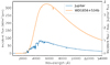 |
Fig. 7 Incident fluxes at the orbits of Jupiter and WD 1856+534 b. |
5 Conclusions
We have obtained multi-colour and low-resolution spectroscopic observations of six transits of WD 1856+534 b, obtaining a transmission spectrum that is essentially flat. Under the assumption that the transmission spectrum is dominated by an undetected Rayleigh scattering, the absence of a significant slope allows us to obtain lower limits to its mass of 4.4, 2.4, and 1.6 MJup at the 1σ, 2σ, and 3σ levels, respectively. These mass limits would favour a common envelope origin for the current orbit of WD 1856+534 b and disfavour other proposed mechanisms, such as the ZKL mechanism or dynamical scattering from additional planets. As an alternative, high-altitude haze layers may be present, which would imply flatter-sloped transmission spectra, in which case corresponding mass limits would be a few times smaller. High clouds could also cause a flat transmission spectrum, but, in a cold object such as WD 1856+534 b, such a spectrum is more likely dominated by hazes.
The average out-of-eclipse spectrum shows previously undetected Hα absorption in the atmosphere of the host WD, which indicates a DA type. We fitted a grid of synthetic spectra of DA WDs to this single line and obtained values of its effective temperature and gravity that are in reasonable agreement with those obtained from an analysis of the SED. We additionally refined the ephemeris of the transits and have shown that the achieved precision will allow for a search of other potential giant planets in the system by means of the LITE during a longer-term observing campaign.
Acknowledgements
We thank the anonymous referee for useful comments that helped to improve the paper. We thank F. Murgas for kindly providing the GTC Sloan g raw data used in V20. R.A. acknowledges funding from the Spanish Research Agency (AEI) of the Ministry of Science and Innovation (MICINN) and the European Regional Development Fund (FEDER) under the grant PGC2018-098153-B-C31. P.R.-G. acknowledges funding from the same agencies under grant AYA2017-83383-P and HJD under grants ESP2017-87676-C5-4-R and PID2019-107061GB-C66, DOI: 10.13039/50110001103. P.I. acknowledges financial support from the Spanish Ministry of Economy and Competitiveness (MINECO) under the 2015 Severo Ochoa Programme MINECO SEV–2015–0548. This publication made use of VOSA, developed under the Spanish Virtual Observatory project supported from the Ministry of Science and Innovation (MICINN) through grant AYA2017-84089. HiPERCAM is funded by the European Research Council under the European Union’s Seventh Framework Programme (FP/2007–2013) under ERC-2013-ADG Grant Agreement no. 340040 (HiPERCAM). This research made use of exoplanet (Foreman-Mackey et al. 2020) and its dependencies (Agol et al. 2020; Kumar et al. 2019; Astropy Collaboration 2013, 2018; Kipping 2013; Luger et al. 2019; Salvatier et al. 2016; The Theano Development Team 2016). This work has made use of data from the European Space Agency (ESA) mission Gaia (https://www.cosmos.esa.int/gaia), processed by the Gaia Data Processing and Analysis Consortium (DPAC, https://www.cosmos.esa.int/web/gaia/dpac/consortium). Funding for the DPAC has been provided by national institutions, in particular the institutions participating in the Gaia Multilateral Agreement. We acknowledge the use of Tom Marsh’s PAMELA.
Appendix A Corner plots
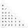 |
Fig. A.1 Corner plots of the fit to the broadband Sloan g photometry. |
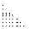 |
Fig. A.2 Corner plots of the fit to the broadband Sloan i photometry. |
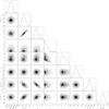 |
Fig. A.3 Corner plots of the fit to the broadband EMIR J photometry. |
References
- Agol, E. 2011, ApJ, 731, L31 [NASA ADS] [CrossRef] [Google Scholar]
- Agol, E., & Fabrycky, D. C. 2018, in Handbook of Exoplanets, eds. H. J. Deeg, & J. A. Belmonte, 7 [Google Scholar]
- Agol, E., Luger, R., & Foreman-Mackey, D. 2020, AJ, 159, 123 [Google Scholar]
- Alonso, R., Barbieri, M., Rabus, M., et al. 2008, A&A, 487, L5 [NASA ADS] [CrossRef] [EDP Sciences] [Google Scholar]
- Alonso, R., Rappaport, S., Deeg, H. J., & Palle, E. 2016, A&A, 589, A6 [NASA ADS] [CrossRef] [EDP Sciences] [Google Scholar]
- Astropy Collaboration (Robitaille, T. P., et al.) 2013, A&A, 558, A33 [NASA ADS] [CrossRef] [EDP Sciences] [Google Scholar]
- Astropy Collaboration (Price-Whelan, A. M., et al.) 2018, AJ, 156, 123 [Google Scholar]
- Bédard, A., Bergeron, P., Brassard, P., & Fontaine, G. 2020, ApJ, 901, 93 [Google Scholar]
- Blouin, S., Dufour, P., & Allard, N. F. 2018, ApJ, 863, 184 [NASA ADS] [CrossRef] [Google Scholar]
- Borucki, W. J., Koch, D., Basri, G., et al. 2010, Science, 327, 977 [NASA ADS] [CrossRef] [PubMed] [Google Scholar]
- Cepa, J., Aguiar, M., Escalera, V. G., et al. 2000, in SPIE Conf. Ser., 4008, Optical and IR Telescope Instrumentation and Detectors, ed. M. Iye & A. F. Moorwood, 623 [Google Scholar]
- de Wit, J., & Seager, S. 2013, Science, 342, 1473 [Google Scholar]
- Dhillon, V., Dixon, S., Gamble, T., et al. 2018, in SPIE Conf. Ser., 10702, Ground-based and Airborne Instrumentation for Astronomy VII, 107020L [Google Scholar]
- Farihi, J. 2016, New Astron. Rev., 71, 9 [NASA ADS] [CrossRef] [Google Scholar]
- Foreman-Mackey, D., Hogg, D. W., Lang, D., & Goodman, J. 2013, PASP, 125, 306 [Google Scholar]
- Foreman-Mackey, D., Luger, R., Czekala, I., et al. 2020, https://doi.org/10.5281/zenodo.3785072 [Google Scholar]
- Gaia Collaboration (Prusti, T., et al.) 2016, A&A, 595, A1 [NASA ADS] [CrossRef] [EDP Sciences] [Google Scholar]
- Gaia Collaboration (Brown, A. G. A., et al.) 2021, A&A, 649, A1 [NASA ADS] [CrossRef] [EDP Sciences] [Google Scholar]
- Gänsicke, B. T., Schreiber, M. R., Toloza, O., et al. 2019, Nature, 576, 61 [NASA ADS] [CrossRef] [Google Scholar]
- Gary, B. L., Rappaport, S., Kaye, T. G., Alonso, R., & Hambschs, F. J. 2017, MNRAS, 465, 3267 [Google Scholar]
- Garzón, F., Castro, N., Insausti, M., et al. 2016, in SPIE Conf. Ser., 9908, Ground-based and Airborne Instrumentation for Astronomy VI, ed. C. J. Evans, L. Simard, & H. Takami, 99081J [Google Scholar]
- Gelman, A., & Rubin, D. B. 1992, Stat. Sci., 7, 457 [Google Scholar]
- Gianninas, A., Strickland, B. D., Kilic, M., & Bergeron, P. 2013, ApJ, 766, 3 [NASA ADS] [CrossRef] [Google Scholar]
- Guerlet, S., Spiga, A., Delattre, H., & Fouchet, T. 2020, Icarus, 351, 113935 [Google Scholar]
- Hoffman, M. D., & Gelman, A. 2014, J. Mach. Learn. Res., 15, 1593 [Google Scholar]
- Howe, A. R., & Burrows, A. S. 2012, ApJ, 756, 176 [NASA ADS] [CrossRef] [Google Scholar]
- Irwin, J. B. 1959, AJ, 64, 149 [NASA ADS] [CrossRef] [Google Scholar]
- Izquierdo, P., Rodríguez-Gil, P., Gänsicke, B. T., et al. 2018, MNRAS, 481, 703 [NASA ADS] [CrossRef] [Google Scholar]
- Karalidi, T., Stam, D. M., & Guirado, D. 2013, A&A, 555, A127 [NASA ADS] [CrossRef] [EDP Sciences] [Google Scholar]
- Kipping, D. M. 2013, MNRAS, 435, 2152 [Google Scholar]
- Kipping, D. M., Torres, G., Henze, C., et al. 2016, ApJ, 820, 112 [NASA ADS] [CrossRef] [Google Scholar]
- Koester, D. 2010, Mem. Soc. Astron. It., 81, 921 [NASA ADS] [Google Scholar]
- Koester, D., Gänsicke, B. T., & Farihi, J. 2014, A&A, 566, A34 [NASA ADS] [CrossRef] [EDP Sciences] [Google Scholar]
- Kozai, Y. 1962, AJ, 67, 591 [Google Scholar]
- Kumar, R., Carroll, C., Hartikainen, A., & Martin, O. 2019, J. Open Source Softw., 4, 1143 [Google Scholar]
- Lagos, F., Schreiber, M. R., Zorotovic, M., et al. 2021, MNRAS, 501, 676 [Google Scholar]
- Lallement, R., Capitanio, L., Ruiz-Dern, L., et al. 2018, A&A, 616, A132 [NASA ADS] [CrossRef] [EDP Sciences] [Google Scholar]
- Lidov, M. L. 1962, Planet. Space Sci., 9, 719 [Google Scholar]
- López-Puertas, M., Montañés-Rodríguez, P., Pallé, E., et al. 2018, AJ, 156, 169 [Google Scholar]
- Luger, R., Agol, E., Foreman-Mackey, D., et al. 2019, AJ, 157, 64 [NASA ADS] [CrossRef] [Google Scholar]
- Maldonado, R. F., Villaver, E., Mustill, A. J., Chávez, M., & Bertone, E. 2021, MNRAS, 501, L43 [Google Scholar]
- Manser, C. J., Gänsicke, B. T., Eggl, S., et al. 2019, Science, 364, 66 [Google Scholar]
- Marsh, T. R. 1989, PASP, 101, 1032 [NASA ADS] [CrossRef] [Google Scholar]
- Marsh, T. R. 2018, in Handbook of Exoplanets, eds. H. J. Deeg, & J. A. Belmonte, 96 [Google Scholar]
- McCook, G. P., & Sion, E. M. 1999, ApJS, 121, 1 [NASA ADS] [CrossRef] [Google Scholar]
- Montañés-Rodríguez, P., González-Merino, B., Pallé, E., López-Puertas, M., & García-Melendo, E. 2015, ApJ, 801, L8 [NASA ADS] [CrossRef] [Google Scholar]
- Muñoz, D. J., & Petrovich, C. 2020, ApJ, 904, L3 [Google Scholar]
- O’Connor, C. E., Liu, B., & Lai, D. 2021, MNRAS, 501, 507 [Google Scholar]
- Pryor, W. R., & Hord, C. W. 1991, Icarus, 91, 161 [NASA ADS] [CrossRef] [Google Scholar]
- Rappaport, S., Gary, B. L., Kaye, T., et al. 2016, MNRAS, 458, 3904 [NASA ADS] [CrossRef] [Google Scholar]
- Rebassa-Mansergas, A., Solano, E., Xu, S., et al. 2019, MNRAS, 489, 3990 [Google Scholar]
- Ricker, G. R., Winn, J. N., Vanderspek, R., et al. 2015, J. Astron. Telescopes Instrum. Syst., 1, 014003 [Google Scholar]
- Robinson, T. D., Maltagliati, L., Marley, M. S., & Fortney, J. J. 2014, Proc. Natl. Acad. Sci. U.S.A., 111, 9042 [Google Scholar]
- Salvatier, J., Wiecki, T. V., & Fonnesbeck, C. 2016, PeerJ Comput. Sci., 2, e55 [Google Scholar]
- Stephan, A. P., Naoz, S., & Gaudi, B. S. 2020, arXiv e-prints, [arXiv:2010.10534] [Google Scholar]
- The Theano Development Team (Al-rfou, R., et al.) 2016, arXiv e-prints, [arXiv:1605.02688] [Google Scholar]
- Tremblay, P. E., Bergeron, P., & Gianninas, A. 2011, ApJ, 730, 128 [NASA ADS] [CrossRef] [Google Scholar]
- Tribbett, P. D., Robinson, T. D., & Koskinen, T. T. 2020, arXiv e-prints, [arXiv:2006.14670] [Google Scholar]
- Vanderbosch, Z., Hermes, J. J., Dennihy, E., et al. 2020, ApJ, 897, 171 [Google Scholar]
- Vanderburg, A., Johnson, J. A., Rappaport, S., et al. 2015, Nature, 526, 546 [NASA ADS] [CrossRef] [Google Scholar]
- Vanderburg, A., Rappaport, S. A., Xu, S., et al. 2020, Nature, 585, 363 [Google Scholar]
- von Zeipel H. 1910, Astron. Nachr., 183, 345 [CrossRef] [Google Scholar]
- West, R. A. 2018, Temperature, Clouds, and Aerosols in Giant and Icy Planets, eds. H. J. Deeg, & J. A. Belmonte, 49 [Google Scholar]
- West, R. A., & Smith, P. H. 1991, Icarus, 90, 330 [NASA ADS] [CrossRef] [Google Scholar]
- Zhang, X., West, R. A., Banfield, D., & Yung, Y. L. 2013, Icarus, 226, 159 [NASA ADS] [CrossRef] [Google Scholar]
- Zuckerman, B., Koester, D., Reid, I. N., & Hünsch, M. 2003, ApJ, 596, 477 [NASA ADS] [CrossRef] [Google Scholar]
- Zuckerman, B., Melis, C., Klein, B., Koester, D., & Jura, M. 2010, ApJ, 722, 725 [Google Scholar]
All Tables
Derived parameters of WD 1856+534 from the photometry (Pan-STARRS1, 2MASS, WISE bands 1 and 2, and Gaia eDR3 blue and red bands), using different thresholds (Errmin) for the minimum uncertainties in the input magnitudes.
Derived parameters of WD 1856+534 b in the three high-cadence light curves and assuming a circular orbit.
All Figures
|
Fig. 1 Light curves of WD 1856+534 obtained with GTC in three different filters. In the right panel, the curves are plotted introducing vertical offsets (to observe the cadence and precision of each of the datasets) and also show the residuals of the best-fit model. The dispersions of the residuals in each colour are 0.6, 0.4, and 0.9%, respectively. |
| In the text | |
|
Fig. 2 Average out-of-transit normalised spectrum of the night of May 20, 2020 centred at the Hα absorption line. The best-fit spectroscopic model of a DA WD is overplotted as a red line, and the model that best fits the photometric data as a blue line. |
| In the text | |
|
Fig. 3 Average out-of-transit spectrum of WD 1856+534 with the wavelength bins used to compute the transmission spectrum. The limits of the bins are represented with vertical blue lines, and the central wavelengths of each bin are indicated at the top with short vertical green lines. The definition of the bins took the locations of the telluric absorption bands into account (marked with the grey bands; these are discarded), and narrower bins were used when the flux was higher. The positions of the Na I doublet and the Hα absorption line are marked with vertical dashed red lines. |
| In the text | |
|
Fig. 4 Transmission spectrum of WD 1856+534 b. The radius of the WD is fixed to the estimated average value (0.0123 R⊙), and the impact parameter is held fixed at a given value (8.5) as both parameters are independent of the wavelength. The larger filled circles mark the radius of the secondary in the Sloan g (cyan), Sloan i (green), and EMIR J (red) filters, while dark blue dots mark the radii determined at each spectral bin defined in Fig. 3. The solid blue lines in the background are random samples of the posterior of the linear fits to measure the atmospheric scale height. We note the logarithmic scale in the x-axis. The verticalscale on the right side gives the difference in kilometres from the mean radius of the secondary. |
| In the text | |
|
Fig. 5 Histogram of the scale heights obtained from the fits to the slope of the transmission spectrum shown in Fig. 4. |
| In the text | |
|
Fig. 6 O–C values of the mid-transit times for which a precision of less than 1 s could be achieved. The lines are random samples of the posterior of a linear fit to these values. |
| In the text | |
|
Fig. 7 Incident fluxes at the orbits of Jupiter and WD 1856+534 b. |
| In the text | |
|
Fig. A.1 Corner plots of the fit to the broadband Sloan g photometry. |
| In the text | |
|
Fig. A.2 Corner plots of the fit to the broadband Sloan i photometry. |
| In the text | |
|
Fig. A.3 Corner plots of the fit to the broadband EMIR J photometry. |
| In the text | |
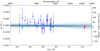 |
Fig. A.4 Same as Fig. 4 but for the night of May 10, 2020. |
| In the text | |
Current usage metrics show cumulative count of Article Views (full-text article views including HTML views, PDF and ePub downloads, according to the available data) and Abstracts Views on Vision4Press platform.
Data correspond to usage on the plateform after 2015. The current usage metrics is available 48-96 hours after online publication and is updated daily on week days.
Initial download of the metrics may take a while.