© ESO 2021

1. Introduction

The widely accepted Λ cold dark matter (ΛCDM) model is very successful in reproducing the large-scale structure of the Universe (e.g., Davis et al. 1985), but it faces some key problems on small scales (e.g., Bullock & Boylan-Kolchin 2017). For example, on the scales of individual galaxies, we observe much less substructure than what is predicted by dark-matter-only (CDM-only) cosmological simulations (Klypin et al. 1999; Moore et al. 1999). These simulations show that substructure exists down to very small scales and can be found at all radii, although preferentially in larger numbers in the outskirts of galaxy halos (e.g., Diemand et al. 2008; Springel et al. 2008).

Several possibilities exist to solve this missing substructure conundrum. For example, adding baryonic physics to the simulations alleviates some of the problems, although mostly in the inner part of galaxies (e.g., D’Onghia et al. 2010; Zhu et al. 2016; Sawala et al. 2017). Adjusting the properties of the dark matter particle (e.g., self-interacting dark matter, warm dark matter, or fuzzy dark matter) can help to suppress the formation of the smallest substructures (e.g., Spergel & Steinhardt 2000; Hu et al. 2000; Bode et al. 2001; Vogelsberger et al. 2016; Bozek et al. 2016; Hui et al. 2017). Another solution is to assume that the structures are present, but in a dark form. Dark structures only reveal their presence through gravitational interaction, rendering them very difficult to detect. Results from gravitational lensing support the existence of dark structures at a level that is compatible with ΛCDM (Dalal & Kochanek 2002; Vegetti et al. 2010, 2012; Ritondale et al. 2019; Hsueh et al. 2020).

Establishing whether a population of subhalos with masses < 10⁸ M_⊙ in and around the Galaxy exists is therefore of the utmost importance as it can lead to a better understanding of the nature of the dark matter particle. Clearly, the discrepancy between the predicted and observed small-scale structure might indicate a fundamental problem with our current cosmological paradigm.

In this work, we focus on a method for indirectly detecting dark subhalos in our own Galaxy through their possible interactions with cold stellar streams. These streams are thin, almost one-dimensional (1D) elongated structures consisting of stars that originate from the tidal disruption of globular clusters or small dwarf galaxies. Because of their fragile nature, these streams are easily perturbed by gravitational interactions, making them promising probes of dark substructures (Ibata et al. 2002; Johnston et al. 2002). Occasional flybys of dark subhalos can create a gap in an otherwise relatively smooth distribution of stars (Yoon et al. 2011; Carlberg 2013). Unfortunately, it is challenging to find streams because their surface brightness is low, and finding gaps in streams is even more difficult. However, recent deep photometric surveys have identified a few dozen narrow streams (e.g., Belokurov et al. 2006; Bernard et al. 2016; Shipp et al. 2018). The analysis of Gaia DR2 (Gaia Collaboration 2016, 2018) has also yielded another dozen streams (Malhan et al. 2018; Ibata et al. 2019). So far, only two of these streams have been claimed to contain gaps: GD-1 (Grillmair & Dionatos 2006) and Palomar 5 (or Pal 5, Odenkirchen et al. 2001), although several other streams show peculiarities (Bonaca et al. 2019a; Shipp et al. 2019; Li et al. 2021).

GD-1 is a promising stream to probe for gaps because of its length and coldness. It is known to contain several non-smooth features (Carlberg & Grillmair 2013; De Boer et al. 2018; Price-Whelan & Bonaca 2018). The origin of these features, or gaps, is currently highly debated in the literature. For example, they could have been formed by an interaction with a massive (dark) object of 10⁶ − 10⁸ M_⊙ that might once have been part of the Sagittarius system (Bonaca et al. 2019b, 2020, see also Banik et al. 2021). On the other hand, it has been argued that the presence and nature of a nearly periodic spatial distribution of gaps is an indication that they might be explained by internal dynamics without the need to recur to interactions with dark structures (Ibata et al. 2020).

The stream of Pal 5 has been tentatively shown to host two gaps and several other features that would be consistent with being induced by subhalos in the range of 10⁶ − 10⁸ M_⊙ (Erkal et al. 2017; Bovy et al. 2017). The inferred number of interactions appears to agree with the expected number predicted by CDM-only simulations (e.g., Sanderson et al. 2016). Unfortunately, the stream of Pal 5 is not ideally suited to search for gaps caused by dark structures because of its proximity to the Galactic centre. The high baryon density in this region can lead to the formation of irregularities in the stream profile, for example, through interactions with the bar (Pearson et al. 2017), globular clusters, and other baryonic structures (Banik & Bovy 2018). Moreover, some of the gaps and features found in the stream of Pal 5 may be explained by survey incompleteness (Thomas et al. 2016).

Because the expectation is that in the near future, many gaps in many different streams will be detected, it is imperative to develop an in-depth understanding of the characteristics and evolution of these gaps. With this understanding we may be able to link the population of gaps to an underlying population of dark substructures. For example, we need to establish the relation between subhalos and gap sizes, the growth rate of gaps, and the dependence of their properties on the encounter parameters as well as on the characteristics of the host potential. Clearly, the ultimate goal would be to infer the properties of the perturbers from the analysis of the observed gaps.

Erkal & Belokurov (2015a) developed a framework that predicts the evolution of gaps formed in streams that orbit on circular orbits. Using this model, Erkal & Belokurov (2015b) inferred the properties of a subhalo from the properties of a gap, down to a degeneracy in subhalo mass and relative velocity. A more recent model by Sanders et al. (2016) focuses on modelling gaps in angle-frequency space, allowing for eccentric orbits (see also Bovy et al. 2017). The authors validated several but not all aspects of Erkal & Belokurov (2015a), and argued, for example, that the velocity dispersions in the underlying stream affect the evolution of the gap and thus should be taken into account. A caveat of all these models is that they are not fully analytical and thus always rely on numerical exploration of the parameter space, or they are limited to circular orbits alone. For this reason, we presented a fully analytical model for the evolution of gaps in streams (Helmi & Koppelman 2016, HK16 hereafter) orbiting in spherical potentials.

In this work, we extend the HK16 model to streams orbiting in axisymmetric potentials. The model presented here not only predicts the behaviour of the size of the gap as a function of time, but also its central density and their dependence on the characteristic parameters of the encounter. This paper is structured as follows. In Sect. 2 we describe the model and its predictions for the gap properties in detail. In Sect. 3 we validate our model with N-body experiments. Subsequently, in Sect. 4 we analyse the dependences of the gap properties on the collision parameters and investigate possible degeneracies in the parameters. Finally, we present a discussion and conclusions in Sect. 5.

2. Methods

The main reason to extend our HK16 model, which only works for spherical potentials, is that the Milky Way is more realistically described as an axisymmetric system. From a dynamical point of view, breaking the spherical symmetry will add a degree of freedom to the system.

The notation we use here is very similar to that employed in HK16. It builds on the action-angle stream description of Helmi & White (1999, HW99 hereafter), see also Helmi & Gomez (2007).

2.1. Choice of the potential

We are somewhat restricted in our choice for a potential for the Milky Way because our approach is based on the use of action-angle variables. These can only be calculated in potentials that are separable in the coordinates. For this reason, we use Stäckel potentials, which are separable in ellipsoidal coordinates and are fully integrable (they are the only type of potentials with this property).

Because the (inner part of the) Milky Way is best described as an oblate system, we use a set of prolate spheroidal coordinates (λ, ϕ, ν) that we adopt from de Zeeuw (1985). The coordinate ϕ is the azimuthal angle and the other two coordinates, λ and ν, are the roots for τ in

$$\begin{array}{c}\hfill \frac{R^2}{\tau +\alpha }+\frac{z^2}{\tau +\gamma }=1,\end{array}$$(1)

where R = x² + y², and α and γ are constants related to the shape of the spheroid. The most general form of a Stäckel potential in these coordinates is

$$\begin{array}{c}\hfill \mathrm{\Phi }(\lambda ,\nu )=\frac{(\nu +\gamma )G(\nu )-(\lambda +\gamma )G(\lambda )}{\lambda -\nu },\end{array}$$(2)

where G(τ) determines the exact shape of the potential. For G(τ) we choose a two-component Kuzmin-Kutuzov potential, which takes the following form:

$$\begin{array}{c}\hfill G(\tau )=\frac{G{M}_h}{\sqrt{\tau }+c_h}+\frac{G{M}_d}{\sqrt{\tau -q}+c_d},\end{array}$$(3)

where q is a parameter set by the choice of the different axis ratios for the components taking into account the constraint that the sum remains a Stäckel potential: λ_h − ν_h = λ_d − ν_d, or λ_d = λ_h − q and ν_d = ν_h − q, where

$$\begin{array}{c}\hfill q=c_h^2\frac{{ϵ}_h^2-{ϵ}_d^2}{1-{ϵ}_d^2},\mathrm{with}q\ge 0.\end{array}$$(4)

Here the ratio of the semi-major a and semi-minor c axis ϵ² = α/γ (i.e. the flattening of the system) is a free parameter for each component, where α = −a² and γ = −c². Finally, we define the fraction of the mass of the disc with respect to the total mass as k = M_d/M_tot, with M_tot = M_d + M_h. We refer to Dejonghe & de Zeeuw (1988) for more details on axisymmetric Stäckel potentials.

The resulting potential is therefore described by five parameters, namely the total mass M_tot, the fraction of mass in the disc k, the scale length of the halo component a_h, and the flattening parameters of the halo ϵ_h and disc ϵ_d. Here we set these parameter values to M_tot = 4.0 ⋅ 10¹¹ M_⊙, k = 0.11, a_h = 7.0 kpc, and ϵ_h = 1.02, ϵ_d = 75.0 (which are based on Batsleer & Dejonghe 1994; Famaey & Dejonghe 2003, see also Reino et al. 2021, where two-component Stäckel potentials are fit to several streams around the Milky Way using Gaia DR2). The resulting potential matches the circular velocity curve of the Milky Way reasonably well, as shown in Fig. 1 (solid black line). This can be inferred by comparison to the recently estimated circular velocity curve from Eilers et al. (2019; in blue).

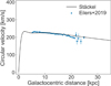Fig. 1. Circular velocity in the plane of the disc of our Milky Way model. The Stäckel potential comprises a disc and a halo component and realistically describes the circular velocity of the Milky Way in the inner ∼20 kpc, as can be seen by comparing to the determinations by Eilers et al. (2019).

2.2. Impulse approximation

Before describing the model, we first describe the effect that a subhalo has on a cold stream. The gravitational interaction of a subhalo is well described by the impulse approximation¹ (Yoon et al. 2011; Carlberg 2013). We define a reference system where the stream is aligned along the y-axis, and moves in the positive y-direction (similar to the system of Erkal & Belokurov 2015a, cf. their Fig. 2). In this co-moving frame the relative velocity vector of the subhalo is w = w(− cos θ sin α, sin θ, cos θ cos α), or w = (−w_⊥ sin α, w_∥, w_⊥ cos α), where w_⊥ = w cos θ and w_∥ = w sin θ. Figure 2 illustrates the geometry of the stream-subhalo encounter.

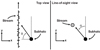Fig. 2. Schematic overview of the stream-subhalo interaction. Left: view seen from the top. Right: view seen along the line of sight (stream away from the observer).

The change in velocity (i.e. the impulse) of a particle along the stream due to the encounter is

$$\begin{array}{c}\hfill \mathrm{\Delta }{v}_i={\displaystyle {\int }_{-\infty }^{\infty }}{a}_i(\mathit{x},\mathit{w},M,r_s)\mathrm{d}t,\end{array}$$(5)

where i = (x, y, z). The acceleration a_i is a function of the relative velocity w, the distance to the point of impact y, and of the subhalo mass M and scale radius r_s. We model the subhalos as Plummer spheres, but the expressions can be generalised for other profiles (Sanders et al. 2016). The change in velocities in all three coordinates at the time of the impulse according to Eq. (5) is

$$\begin{array}{c}\hfill \frac{\mathrm{\Delta }{v}_x}{2GM}=\frac{{\mathit{yw}}_{\perp }{w}_{\Vert }sin\alpha }{w(r_s^2{w}^2+y^2{w}_{\perp }^2)}=\frac{ycos\theta sin\theta sin\alpha }{w(r_s^2+y^2{cos}^2\theta )},\end{array}$$(6a)

$$\begin{array}{c}\hfill \frac{\mathrm{\Delta }{v}_y}{2GM}=-\frac{w_{\perp }^{2}y}{w(r_s^2{w}^2+y^2{w}_{\perp }^2)}=-\frac{y{cos}^2\theta }{w(r_s^2+y^2{cos}^2\theta )},\end{array}$$(6b)

$$\begin{array}{c}\hfill \frac{\mathrm{\Delta }{v}_z}{2GM}=-\frac{{\mathit{yw}}_{\perp }{w}_{\Vert }cos\alpha }{w(r_s^2{w}^2+y^2{w}_{\perp }^2)}=-\frac{ycos\theta sin\theta cos\alpha }{w(r_s^2+y^2{cos}^2\theta )}.\end{array}$$(6c)

The above expressions are valid for direct encounters, that is, when the impact parameter b = 0. Equations (1)–(3) in Erkal & Belokurov (2015a) provide a more general form for the velocity changes that take the parameter b into account. This parameter enters into the equations above through $r_s^2\to r_s^2+b^2$.

We assume that the stream is linear over the scale where the impulse is significant. Moreover, the equations above assume that the stream is a 1D structure. This approximation is sufficient when the width of the stream is smaller than the scale radius of the subhalo. However, the expressions can be generalised to the full 3D case, for which we find

$$\begin{array}{c}\hfill \mathrm{\Delta }{v}_i(\mathit{x})=-\frac{2GM}{w}\frac{w^2{x}_i-w_i(\mathit{x}·\mathit{w})}{(r_s^2+\mathit{x}·\mathit{x})w^2-{(\mathit{x}·\mathit{w})}^2},\end{array}$$(7)

with i = (x, y, z). To gain insight into the model, we use the equations of the 1D approximation in this section. However, when evaluating the model, we use the full 3D equations.

From Eq. (6) we can find the maximum kick in velocities $\mathrm{\Delta }{v}_i^{\max }$ and at what distance y_max to the centre of impact it occurs,

$$\begin{array}{c}\hfill \mathrm{\Delta }{v}_i^{\max }=-\frac{2GM}{w}\frac{w^2{x}_i-w_i{w}_y{y}_{\max }}{(r_s^2+y_{\max }^2)w^2-{(y_{\max }{w}_y)}^2},\end{array}$$(8a)

where x_i = [0, y_max, 0] and

$$\begin{array}{c}\hfill y_{\max }=\frac{w{r}_s}{\sqrt{w^2-w_y^2}}=\frac{r_s}{cos\theta }.\end{array}$$(8b)

Typical profiles of Δv_y(y) are shown and discussed in Sect. 3, see Fig. 11.

2.3. Action-angle variables

This section aims to serve as a brief introduction to these variables, and it is by no means exhaustive or comprehensive. For more details on action-angle variables, we refer to Goldstein et al. (2002) and Binney & Tremaine (2008).

Orbits in smooth and simple potentials (e.g., spherical, axisymmetric, triaxial) have a number of integrals of motion: properties that do not change in time and serve to characterise them. For a spherical potential, the integrals of motion are the total energy (or the Hamiltonian) and the angular momentum vector. Orbits in axisymmetric systems (e.g., disc galaxies) typically have up to three integrals of motion: the total energy, the momentum in the azimuthal direction, and a non-classical integral that in most cases does not take an analytic form.

For separable potentials (e.g., the Stäckel potentials discussed in Sect. 2.1) there exist three isolating integrals J, known as the actions. Each action is paired with a conjugate coordinate θ, the angles. Together, these coordinates make up the action-angle variables (Θ, J). The actions uniquely define the orbit, that is, a point in action-space corresponds to a complete orbit in phase-space. The conjugate angles define the phase, that is, they specify where along the orbit a body is located at any given time.

To obtain the action-angle variables we make use of the Hamiltonian H, which being an integral of motion must depend on the actions (i.e. H = H(J)). The rate of change of the angles $\dot{\mathbf{\Theta }}=\partial H/\partial \mathbf{J}$ is known as the frequency Ω(J). Therefore

$$\begin{array}{c}\hfill \mathbf{\Theta }(t)={\mathbf{\Theta }}_0+\mathbf{\Omega }t,\end{array}$$(9)

and hence the angles are linearly dependent on time. Finally, the actions J of a bound orbit in a separable potential are defined as

$$\begin{array}{c}\hfill \mathbf{J}=\frac{1}{2\pi }{\displaystyle \oint \mathbf{p}}·\mathrm{d}\mathbf{q},\end{array}$$(10)

where (q, p) are any set of generalised phase-space coordinates and momenta.

2.4. Size of the gap using an action-angle framework

The analytical framework of the method that we use to describe the evolution of a gap in a stream with time, was first established by HW99. Originally, this framework was used to describe the divergence in the orbits of a distribution of nearby particles. It makes use of a linearised Taylor expansion around a central orbit. In our case, we model the size of the gap as the spatial separation of two orbits: one on each side of the gap. These orbits are taken to be those of the particles that receive the largest impulse from the subhalo flyby. In practice, this is equivalent to modelling the (size of the) gap as twice the separation of the central orbit and one of the edges of the gap, as gaps are symmetric with respect to their centre.

2.4.1. Generalities

We consider a central orbit and some other orbit separated by ΔX₀ and ΔV₀, where the subscript is used to denote the time of the impact between the subhalo and the stream, t = t₀. To calculate the evolution of this separation vector, we first transform it to action-angle variables,

$$\begin{array}{c}\hfill \left[\begin{array}{c}\mathrm{\Delta }{\mathbf{\Theta }}_0\\ \mathrm{\Delta }{\mathbf{J}}_0\end{array}\right]={\mathcal{M}}_0\left[\begin{array}{c}\mathrm{\Delta }{\mathbf{X}}_0\\ \mathrm{\Delta }{\mathbf{V}}_0\end{array}\right],\end{array}$$(11)

where ℳ₀ is a matrix calculated at t = t₀ that locally transforms from Cartesian coordinates to action-angle variables. In practice, the transformation is a product of matrices,

$$\begin{array}{c}\hfill {\mathcal{M}}_0={\mathcal{M}}_0^{\mathrm{AA}\leftarrow \mathrm{st}}{\mathcal{M}}_0^{\mathrm{st}\leftarrow \mathrm{cyl}}{\mathcal{M}}_0^{\mathrm{cyl}\leftarrow \mathit{xyz}},\end{array}$$(12)

where ${\mathcal{M}}_0^{\beta \leftarrow \alpha }$ transforms the set of coordinates α to the set β, _xyz indicating Cartesian coordinates, _cyl cylindrical coordinates, _st spheroidal coordinates used for the Stäckel potential, and _AA action-angle variables.

Next, the separation vector in action-angle variables can be evolved in time by expanding linearly Eq. (9) and making use of the matrix Ω′,

$$\begin{array}{c}\hfill {\mathrm{\Omega }}^{\prime }=\left[\begin{array}{cc}{I}_3& \partial \mathbf{\Omega }/\partial \mathbf{J}t\\ 0& I_3\end{array}\right].\end{array}$$(13)

At any point in time, the separation in action-angle coordinates can be transformed back to Cartesian coordinates locally, and therefore

$$\begin{array}{c}\hfill \left[\begin{array}{c}\mathrm{\Delta }{\mathit{X}}_t\\ \mathrm{\Delta }{\mathit{V}}_t\end{array}\right]={\mathcal{M}}_t^{-1}{\mathrm{\Omega }}^{\prime }{\mathcal{M}}_0\left[\begin{array}{c}\mathrm{\Delta }{\mathbf{X}}_0\\ \mathrm{\Delta }{\mathbf{V}}_0\end{array}\right],\end{array}$$(14)

where ${\mathcal{M}}_t^{-1}$ is the (local) transformation back to Cartesian coordinates at time t and at the location of the central orbit of the gap.

Finally, the size of the gap can be taken as twice the separation calculated in Eq. (14). The initial separation of the two orbits describing the gap can be obtained assuming Eqs. (8a) and (8b). Because the two orbits are typically separated a few kiloparsec initially, we need to add the velocity gradient of the orbit to the separation in velocities, so ΔV₀ = Δv^max + δv_orbit. We note that this is an ad hoc fix to the non-local nature (finite extent) of the stream. It takes into account that the velocity of the stream particles changes as a function of location.

2.4.2. Long-term behaviour

The growth rate of the size of the gap can be derived from Eq. (14) in a similar fashion as shown in HK16. In the limit where t ≫ t₀ (or better t/t_orb ≫ 1), this equation simplifies to

$$\begin{array}{c}\hfill \left[\begin{array}{c}\mathrm{\Delta }{\mathit{X}}_t\\ \mathrm{\Delta }{\mathit{V}}_t\end{array}\right]\sim t\left[\begin{array}{c}{\mathcal{M}}_{t,1}^{-1}\partial \mathbf{\Omega }/\partial \mathbf{J}\mathrm{\Delta }{\mathbf{J}}_0\\ {\mathcal{M}}_{t,3}^{-1}\partial \mathbf{\Omega }/\partial \mathbf{J}\mathrm{\Delta }{\mathbf{J}}_0\end{array}\right],\end{array}$$(15)

where ${\mathcal{M}}_{t,1}^{-1}$ is the upper left submatrix of ${\mathcal{M}}_t^{-1}$, and ${\mathcal{M}}_{t,3}^{-1}$ is the bottom left submatrix. The spatial separation of the two orbits is equal to the length of vector ΔX_t,

$$\begin{array}{c}\hfill |\mathrm{\Delta }{\mathit{X}}_t|=\sqrt{\mathrm{\Delta }{\mathit{X}}_t^{†}\mathrm{\Delta }{\mathit{X}}_t}\sim t\sqrt{\mathrm{\Delta }{\mathbf{J}}_0^{†}{f}_{\mathit{x},\mathbf{\Omega }}\mathrm{\Delta }{\mathbf{J}}_0}.\end{array}$$(16)

In this equation, $f_{\mathit{x},\mathbf{\Omega }}=\partial \mathbf{\Omega }/\partial \mathbf{J}{{\mathcal{M}}_{t,1}^{-1}}^{†}{\mathcal{M}}_{t,1}^{-1}\partial \mathbf{\Omega }/\partial \mathbf{J}$. Similarly, we can calculate the velocity difference of the two orbits ΔV_t,

$$\begin{array}{c}\hfill |\mathrm{\Delta }{\mathit{V}}_t|=\sqrt{\mathrm{\Delta }{\mathit{V}}_t^{†}\mathrm{\Delta }{\mathit{V}}_t}\sim t\sqrt{\mathrm{\Delta }{\mathbf{J}}_0^{†}{f}_{\mathit{v},\mathbf{\Omega }}\mathrm{\Delta }{\mathbf{J}}_0},\end{array}$$(17)

where $f_{\mathit{v},\mathbf{\Omega }}=\partial \mathbf{\Omega }/\partial \mathbf{J}{{\mathcal{M}}_{t,3}^{-1}}^{†}{\mathcal{M}}_{t,3}^{-1}\partial \mathbf{\Omega }/\partial \mathbf{J}$.

We note that the terms f_x, Ω and f_v, Ω are dependent on the orbit of the gap and its location, but they do not depend on the impact parameters. Both |ΔX_t| and |ΔV_t| are linearly dependent on time t, similar to gaps orbiting in spherical potentials. Interestingly, the ratio of the two separations is constant with time, which potentially can be used to infer the properties of the gap at any time (as we also demonstrate in Sect. 4).

2.5. Density of stream gaps

We now build further on the framework developed by HW99 and focus on modelling the evolution of the density of the gap. The impulse imparted on the stream by the subhalo increases the local velocity dispersion of the stars in the gap. This causes it to grow faster and thus appear as underdense region in comparison to the neighbouring parts of the stream. If we know the central orbit of the gap and the initial phase-space distribution around it, we can calculate the evolution of the density in the gap.

2.5.1. Generalities

We describe this initial phase-space distribution as a multi-variate Gaussian distribution, in other words

$$\begin{array}{c}\hfill f(\mathit{x},\mathit{v})=f_{0}exp(-\frac{1}{2}{\mathrm{\Delta }}_{\varpi ,0}^{†}{\sigma }_{\varpi ,0}{\mathrm{\Delta }}_{\varpi ,0}),\end{array}$$(18)

where f₀ is the phase-space density at t = t₀, Δ_ϖ, 0 is a separation vector: Δ_ϖ, 0 = ξ_i − ξ_c, i and where ξ_i = [x, y, z, v_x, v_y, v_z] and ξ_c, i is the central point of the distribution (which we take to be the location where the subhalo impacts the stream, or in the terminology used previously, the central orbit) at t = t₀. The matrix σ_ϖ, 0 is the inverse of the covariance matrix of the phase-space coordinates.

To compute the initial dispersion matrix of the gap, we start from the original unperturbed distribution and add the impulse in the velocities according to Eq. (7). That is, we transform ${\sigma }_{\varpi ,0}^{\mathrm{stream}}+\mathrm{impulse}\to {\sigma }_{\varpi ,0}^{\mathrm{gap}}$. Below we show how to calculate the new covariance matrix in the regime where the stream is approximated by a 1D structure, but in Appendix A we provide the full 3D expressions.

The most general form of the initial unperturbed covariance matrix Σ_ϖ, 0 is

$$\begin{array}{c}\hfill {\mathrm{\Sigma }}_{\varpi ,0}={\sigma }_{\varpi ,0}^{-1}=\left(\begin{array}{ccc}{\sigma }_x^2& C(x,y)& \cdots \\ C(y,x)& {\sigma }_y^2& \cdots \\ ⋮& ⋮& \ddots \\ \end{array}\right),\end{array}$$(19)

where C(x, y) is the covariance of x and y and σ_x is the standard deviation of x. The covariance matrix can be represented with 3 × 3 block matrices,

$$\begin{array}{c}\hfill {\mathrm{\Sigma }}_{\varpi ,0}=\left(\begin{array}{cc}{\mathbb{C}}_{\mathit{x},\mathit{x}}& {\mathbb{C}}_{\mathit{x},\mathit{v}}\\ {\mathbb{C}}_{\mathit{v},\mathit{x}}& {\mathbb{C}}_{\mathit{v},\mathit{v}}\end{array}\right),\mathrm{where}{\mathbb{C}}_{\mathit{x},\mathit{v}}={\mathbb{C}}_{\mathit{v},\mathit{x}}^{†}.\end{array}$$(20)

We now proceed to compute the perturbed covariance matrix by computing the changes of each individual element due to the encounter with the subhalo. The impulse only affects the velocities. Therefore the position block matrix (ℂ_x, x) does not change during the encounter. The first element with a velocity term is in the ℂ_x, v block matrix,

$$\begin{array}{c}\hfill C(v_x,x)=\frac{1}{n}{\displaystyle \sum _{i=1}^n}(v_{x_i}-{\mathrm{\mu }}_{v_x})(x_i-{\mathrm{\mu }}_x),\end{array}$$(21)

where n is the total number of particles, and μ_vx and μ_x are the mean v_x and x of the distribution in the region around the gap. After applying the impulse, the new covariance element becomes

$$\begin{array}{c}\hfill C(v_x+\mathrm{\Delta }{v}_x,x)=\frac{1}{n}{\displaystyle \sum _{i=1}^n}(v_{x_i}+\mathrm{\Delta }{v}_{x_i}-{\mathrm{\mu }}_{v_x}-\mathrm{\Delta }{\mathrm{\mu }}_{v_x})(x_i-{\mathrm{\mu }}_x),\end{array}$$(22)

where Δv_xi is the velocity change of particle i, and Δμ_vx is the shift of the mean velocity of all particles. Because the kicks are symmetric around the central point, the mean shift of velocities is zero Δμ_vx = 0, and we can rewrite the covariance term as

$$\begin{array}{c}\hfill C(v_x+\mathrm{\Delta }{v}_x,x)=C(v_x,x)+\frac{1}{n}{\displaystyle \sum _{i=1}^n}\mathrm{\Delta }{v}_{x_i}(x_i-{\mathrm{\mu }}_x).\end{array}$$(23)

Considering that the covariance matrix describes the central density (i.e. positions close to the centre), we can express the kick Δv_x as a function that is only linearly dependent on y because the quadratic term in the denominator of Eq. (6a) is negligible (i.e. $r_s^2{\mathit{w}}^2\gg {\mathit{y}}^2{\mathit{w}}_{\perp }^2$). Moreover, because the velocity kicks are calculated in a frame where there is symmetry with respect to y (i.e. μ_y = 0), we can rewrite the last term in the equation above as

$$\begin{array}{c}\hfill \frac{1}{n}{\displaystyle \sum _{i=1}^n}\mathrm{\Delta }{v}_{x_i}(x_i-{\mathrm{\mu }}_x)=2GM\frac{w_{\perp }{w}_{\Vert }sin\alpha }{r_s^2{w}^3}\frac{1}{n}{\displaystyle \sum _{i=1}^n}(y_i-{\mathrm{\mu }}_y)(x_i-{\mathrm{\mu }}_x),\end{array}$$(24)

which is equal to

$$\begin{array}{c}\hfill C(v_x+\mathrm{\Delta }{v}_x,x)=C(v_x,x)+2GM\frac{w_{\perp }{w}_{\Vert }sin\alpha }{r_s^2{w}^3}C(y,x).\end{array}$$(25)

The new covariance term C(v_x + Δv_x, x) can be expressed as the old covariance term plus a new term that depends on the impact parameters. The procedure shown above can be extended to all covariance terms of the form C(α, v_β + Δv_β) and C(v_β + Δv_β, α), where (α, β)=(x, y, z).

Using similar arguments, it is easy to show that covariance terms in the velocity submatrix (ℂ_v, v) take the following general form:

$$\begin{array}{cc}& C(v_{\alpha }+\mathrm{\Delta }{v}_{\alpha },v_{\beta }+\mathrm{\Delta }{v}_{\beta })=C(v_{\alpha },v_{\beta })+C(\mathrm{\Delta }{v}_{\alpha },v_{\beta })\hfill \\ \hfill & +C(v_{\alpha },\mathrm{\Delta }{v}_{\beta })+C(\mathrm{\Delta }{v}_{\alpha },\mathrm{\Delta }{v}_{\beta }).\hfill \end{array}$$(26)

For example, for α = x and β = y, and following similar procedures as above,

$$C(\mathrm{\Delta }{v}_x,v_y)=2GM\frac{w_{\perp }{w}_{\Vert }sin\alpha }{r_s^2{w}^3}C(y,v_y),$$(27)

$$C(v_x,\mathrm{\Delta }{v}_y)=-2GM\frac{w_{\perp }^2}{r_s^2{w}^3}C(v_x,y),$$(28)

$$C(\mathrm{\Delta }{v}_x,\mathrm{\Delta }{v}_y)=-(2\frac{\mathit{GM}}{r_s^2{w}^3}{)}^2{w}_{\perp }^3{w}_{\Vert }sin\alpha C(y,y).$$(29)

We now have full expressions for the matrix σ_ϖ, 0 in Eq. (18) representing the phase-space configuration around the gap at the time of the encounter t = t₀. By transforming σ_ϖ, 0 to action-angle coordinates as ${\sigma }_{\omega ,0}={{\mathcal{M}}_0^{-1}}^{†}{\sigma }_{{\varpi }_0}{\mathcal{M}}_0^{-1}$, where ℳ is the transformation matrix defined in Eqs. (11) and (12), we can calculate the evolution in time of the covariance matrix in phase-space using Eq. (13). This allows us to describe the local density of the portion of the stream around the location of the impact by the subhalo (i.e. of the gap) as

$$\begin{array}{c}\hfill \rho ({\mathit{x}}_c,t)={\displaystyle \int f}({\mathit{x}}_c,\mathit{v},t){\mathrm{d}}^3\mathit{v},\end{array}$$(30)

where ρ(x_c, t) is the density of orbits in a location around the central orbit. In the principal axes, where the velocity covariance matrix is diagonal, this density takes a simple form:

$$\begin{array}{c}\hfill \rho ({\mathit{x}}_c,t)={\rho }_0/\sqrt{det|{\sigma }_v|}\propto {\rho }_0{\sigma }_{v_1}(t){\sigma }_{v_2}(t){\sigma }_{v_3}(t),\end{array}$$(31)

where ρ₀ is the central density at t = t₀ and σ_v1, σ_v2, σ_v3 are the velocity dispersions along the three principal axes.

2.5.2. Long-term behaviour of the density

Using the above formalism, it is possible to show that the density of a stream (and thus also that of a gap) decreases as a power law of time that depends on the number of degrees of freedom of the orbit of the stream (Vogelsberger et al. 2008),

$$\begin{array}{c}\hfill \rho \propto t^{-n},\mathrm{with}n=\mathrm{d}.\mathrm{o}.\mathrm{f}.\end{array}$$(32)

Ultimately, these degrees of freedom are determined by the number of independent frequencies, and this number is generally dependent on the functional form of the potential. For axisymmetric galaxies the number of d.o.f. is 3 for most (non-resonant) orbits. On the other hand, for example, circular orbits only have one degree of freedom, implying that the density decreases much slower (i.e. 1/t).

HW99 derived a general expression for the central density at late times for streams (and gaps) in a general Stäckel potential (see their Appendix C) and found

$$\begin{array}{c}\hfill \rho ({\mathbf{x}}_c,t)=\frac{{\rho }_0{f}_{\mathrm{orb}}}{\sqrt{det|{\sigma }_{{\mathrm{\Theta }}_0}|}}{t}^{-3},\end{array}$$(33)

where ρ₀ is the initial density of the distribution, f_orb is a constant determined by the central orbit, and σ_Θ0 is the angle submatrix at t = t₀. This implies that the ratio of the density of a perturbed to unperturbed stream is a constant,

$$\begin{array}{c}\hfill \delta {\rho }_{\mathrm{str}}^{\mathrm{gap}}=\sqrt{\frac{det{|{\sigma }_{{\mathrm{\Theta }}_0}|}_{\mathrm{str}}}{det{|{\sigma }_{{\mathrm{\Theta }}_0}|}_{\mathrm{gap}}}},\end{array}$$(34)

as all other variables are independent of the impact parameters. We refer below to this density ratio as the density contrast.

2.6. Setting up the stream-subhalo encounter

To verify our model predictions, we performed N-body simulations of the encounter of a subhalo with a stream orbiting in the Milky Way potential described in Sect. 2.1. To this end, we used a modified version of GADGET-2 (Springel 2005), where we modelled the host as the rigid potential and the subhalo as a rigid Plummer sphere that is centred on a particle with a negligible mass that is placed on a trajectory in the host potential.

The progenitor of the stream was modelled with 10⁶ test particles² following a Gaussian distribution in 6D phase space, with σ_x = 0.2 kpc and σ_v = 0.5 km s⁻¹. These very low dispersions were chosen such that the stream has a high density even a few billion years after forming. In comparison, globular clusters orbiting the Milky Way typically have a σ_v of a few km s⁻¹ (e.g., Harris 1996, 2010 edition).

The progenitor was placed on an elongated orbit with maximum distance from the centre r_max ≈ 20 kpc and minimum distance r_min ≈ 10 kpc, reaching r_z = ±20 kpc above the plane of the disc, as shown in Fig. 3. After the progenitor of the stream was evolved for 1 Gyr in the host potential, a subhalo was inserted on a trajectory that directly crosses the stream. We removed the subhalo after the collision to isolate a single interaction and when its gravitational effect was sufficiently small that it no longer affected the stream.

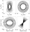Fig. 3. Orbit of the stream shown in galactocentric Cartesian coordinates, evolved for 10 Gyr forward in time in the Stäckel axisymmetric Milky Way-like potential. Top: orbit in coordinates aligned with the host galaxy (e.g., plane of the disc is z = 0). Bottom: coordinates aligned with the initial angular momentum vector of the orbit. The bottom right panel highlights the precession of the orbital plane, which is indicative of the non-spherical nature of the potential considered.

Figure 4 shows an example of a stream-subhalo interaction. The left panel shows both the stream and a subhalo at the time of the collision. The right panels show a stream with and without an encounter 2 Gyr after the interaction with the subhalo. The perturbed stream clearly shows a gap of several kiloparsec in size at the centre of the panel.

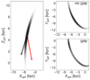Fig. 4. Left: snapshot of a stream at the time of interaction with a subhalo. The stream is plotted with black dots, and the centre of mass of the subhalo is shown as a solid red circle. The velocity vector of the stream is marked with a black arrow and that of the subhalo with a red arrow. Right: both panels show the stream after 2 Gyr of evolution, in isolation in the top panel, and after the encounter with the subhalo in the bottom panel.

3. Results

We compare the predictions of the model presented in Sects. 2.4 and 2.5 with the gaps produced in the N-body experiments. We first investigate gaps produced by subhalos of varying mass and size for a fixed encounter configuration (i.e. the same velocity and impact angle). Next, we focus on the effects of a varying configuration while keeping the subhalo properties fixed.

3.1. Size evolution

Figure 5 shows the evolution of gaps caused by interactions sharing the same configuration, but with different subhalo masses (see Table 1 for their properties). The model (solid lines) reproduces the size of the gap as measured in the N-body simulation very well (coloured dashed lines). The latter is measured as the average separation of two groups of 50 particles on each side of the gap. These 50 particles are identified as those that experience the largest velocity change at the time of the impact. We used 50 particles to lower the effects of discreteness of the N-body simulation, but there is only very little difference when the single particle with the maximum velocity change on each side of the gap is used. The bottom panel of Fig. 5 shows the total distance of the gap to the centre of the host galaxy and gives an indication of its orbit. The frequency of r(t) and the oscillations in the gap size are in antiphase. This is naturally expected because the gap is stretched at pericentre and is smallest at apocentre.

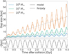Fig. 5. Top panel: gaps growing in a stream orbiting an axisymmetric Stäckel Milky Way-like potential. The lines with different colours show the size of the gaps induced by subhalos of different sizes. The solid curves correspond to our analytic model, and the dashed curves to gaps measured in the N-body experiments. The straight dashed grey lines illustrate the linear growth rate of the gaps. Bottom panel: distance of the central orbit to the centre of the host potential.

Although Fig. 5 shows that the model reproduces the gap size in the N-body experiment very well, there appears to be an upper limit to its measured size. The largest difference is apparent for the encounter with the most massive subhalo at late times. This limit occurs because the size of the gap becomes comparable to the typical scale of the orbit and hence our method of measuring the size of the gap fails to work. The typical scale of the specific orbit we used is ≲40 kpc, see Fig. 6. This value can also be determined analytically using the inverse of Eq. (11) and considering that the two orbits on each side of the gap are at a maximum separation at ΔΘ = π. The maximum distance between two particles on the same orbit but apart by 180° in the angles at any location in the orbit is ∼35 kpc. This value agrees very well with the ceiling reached by the dashed red line measured from the N-body experiment in Fig. 5.

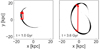Fig. 6. Left: stream 1 Gyr after an interaction with a subhalo. The two red dots indicate the orbits that were used to measure the size of the gap, and the red arrow shows the distance on a straight line between the two dots. Right: same stream 3.6 Gyr after the encounter. At this point in time, the two orbits (red dots) are close to their maximum separation.

The size of the gap in this regime is pushing the limits of our analytical model. The transformation from action-angle variables to Cartesian coordinates (i.e. Eq. (14)) is only valid locally near the central orbit, and therefore the approximation breaks down for such large gaps. Although it should be possible to extend the formalism to include cases like this, this is not really necessary as there are no known streams with gaps of this size, nor is it likely that a gap like this is observed in the (near) future.

3.2. Evolution of the density

Now we compare the density as predicted by our model with the density measured in N-body experiments. For the latter we counted the number of particles in a small volume in 6D space with r <  0.1 kpc and v <  7.5 km s⁻¹. This velocity limit does not remove any particles from the stream at t₀ when the impact occurs, but it removes particles that may have drifted away (i.e. have a different orbital phase) at later times. The volume is centred on the central orbit, which is determined in a simulation of a stream with the same set-up, but without a subhalo interaction.

Figure 7 compares the predicted (solid lines) and measured density from the N-body simulation (dashed lines) for a stream with and without a gap. For the latter, we simulated the exact same stream with and without an encounter with a subhalo. Although the peaks and troughs of the stream and the gap are always larger in our model, the figure shows that the model provides an excellent description of the N-body experiments. The small differences can be attributed to a resolution effect: In the N-body experiments, we measure the density in a finite volume, whereas the model computes a density at a single location in space. If the density were measured in a smaller volume in our experiments, the peaks would be sharper. However, the number of particles would drastically decrease and drop to less than a handful in less than 4 Gyr of evolution.

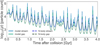Fig. 7. Density evolution of an unperturbed stream (in blue) and of a gap in a stream following the same orbit (in green). The dashed curves are the densities obtained from the corresponding N-body experiments. The agreement between the solid and dashed curves is excellent. The subhalo that is used to create the gap in the stream has a mass of 107 M⊙.

3.2.1. Varying subhalo masses

Next, we explore the evolution of the density contrast (i.e. the ratio of the density around the gap to that of the unperturbed stream) in Fig. 8. The figure shows the same experiments as those plotted in Fig. 5, with the density contrast of the most massive subhalo shown in a separate panel. For the most massive halo, we slightly modified our set-up. Instead of starting from the same initial conditions as the other experiments using the orbit shown in Fig. 3, we used the location of the gap to determine its orbit. We used this as the central orbit both in our analytical model and for the N-body experiment representing the unperturbed stream because when the subhalo and the stream interact, the stream receives an impulse that slightly displaces it from its original orbit. The effect is negligible for subhalos of M ≲ 10⁷ M_⊙ and is small but apparent for more massive objects, particularly after ∼3−4 Gyr of evolution. This new set-up is more realistic because when attempting to model an observed stream or gap, its actual measured position and velocity in a suitable gravitational potential would be integrated (because it is not possible to have a priori access to the original initial conditions of the orbit of the stream before it received the impact).

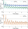Fig. 8. Density contrast measured for a stream experiencing an encounter with subhalos of different mass and scale radius, see Table 1. The relative velocity of the impact is the same for all three interactions. The coloured solid lines show the density contrast according to our model, and the dashed lines are measured in the N-body experiments. The shaded areas indicate the Poisson error in the observed density. The subhalo of 108 M⊙ is shown in a different panel because of its slightly different set-up.

In Fig. 8 we show with solid lines the predicted density contrast from our model and with dashed lines those measured in the N-body experiments. The Poisson errors on the ratio of the densities as measured in the N-body experiments are marked with shaded areas. In general, the amplitude of the density contrast is well reproduced by the model. The difference in the amplitude of the narrow peaks at early times is explained by the same resolution effects as described in Sect. 3.2.

3.2.2. Variation of the encounter configuration

Finally, we verified how our model performs for different configurations of the stream-subhalo encounter, keeping the subhalo at a fixed mass of 10⁷ M_⊙. We compared three different configurations that correspond to rotations of the same velocity vector as listed in Table 2, with Configuration 1 being that used in the previous section. We note that the velocity vector was rotated in the rest frame, not in the co-moving frame of the stream. The resulting configurations thus have different velocity amplitudes in the co-moving frame.

Figures 9 and 10 show the time evolution of the size and density contrast. The layout of the figures is the same as in the previous section. Again, the model (solid lines) predicts the behaviour of the gaps as measured in the N-body experiments (dashed lines) extremely well.

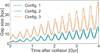Fig. 9. Similar to Fig. 5, but for three different configurations of the stream-subhalo interactions. The gaps of all configurations are created by the same subhalo of size 107 M⊙, but their relative velocity w and impact angles θ and α are different.

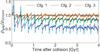Fig. 10. Similar to Fig. 8, but for three different stream-subhalo interactions with a subhalo of fixed mass, and whose size evolution is described in Fig. 9.

Interestingly, Configuration 2 with a subhalo of 10⁷ M_⊙ gives rise to a density contrast of similar amplitude as the collision with the subhalo of 10⁶ M_⊙ (see Fig. 8) in Configuration 1, both producing a gap with a density contrast of ∼0.9. However, when we examine the size of the gaps, we note that the gap caused by the 10⁶ M_⊙ subhalo (blue curve Fig. 5) is smaller than that for the 10⁷ M_⊙. This implies that by measuring both size and density, we may be sensitive to different parameters characterising the encounter, as we discuss in more detail in Sect. 4.

Figure 9 shows that the gaps resulting from the encounter in Configurations 1 and 2 have initially approximately the same size. Interestingly, the gap resulting in Configuration 3 is initially the largest and also remains the largest throughout its evolution in time (although the size is somewhat poorly modelled because the change in velocities for this particular configuration is very shallow, see Fig. 11, which gives rise to some complications in identifying the correct particles to trace in the N-body).

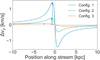Fig. 11. Profile of the change in velocity along the stream vy for the three different configurations described in the two previous figures. In Configuration 1 the stream experiences the largest kick on the smallest scale. On the other hand, in Configuration 3 the kick is much smaller but on a much larger scale. The arrows indicate the location of the maximum Δvy.

On the other hand, Fig. 10 shows that the evolution of the density for Configuration 3 is very similar to that of an unperturbed stream. To understand this, we consider the velocity kicks Δv_y and their profiles as shown in Fig. 11. Because the initial size of the gap is derived from the location of the maximum velocity change, the gap that is initially produced in Configuration 3 is much larger than the other two. Comparing Figs. 10 and 11, we see that the steepest density contrast is associated with the largest change in velocity, exactly as expected. These results imply that the size of the gap is strongly correlated with the distance between the maximum velocity change, whereas the density contrast is more correlated with the amplitude of the change (see also the expressions in the next section).

4. Exploration of the gap observables: dependences and degeneracies

After validating our analytic model, we used it to explore the dependence of the size and density of a gap on the collision parameters using Eqs. (16) and (33). We considered hypothetical gaps formed in the stream presented in Sect. 2.6 and analysed in Sect. 3. To this end, we varied the characteristic parameters of the collision with a subhalo, namely w, θ, and M, while keeping the angle α fixed at some arbitrary value α = 163°. We considered w in the range [0, 800] km s⁻¹ and θ in the range [−90° ,90°]. Instead of separately varying M and r_s, we used a relation for V_max ∝ r_max for subhalos found in the Aquarius simulations by Springel et al. (2008), see Appendix B for details.

Figure 12 shows the gap properties, namely size and density contrast, as a function of these characteristic parameters. Each panel shows the dependence of these two observable quantities with one of the three parameters: M, w, or sin θ. At the same time, we discretely varied a second parameter that gives rise to the different curves in each subpanel, but kept the third parameter fixed. For example, in the leftmost panels we show the variation in gap size (top) and density contrast (bottom) 2.5 Gyr after impact as a function of mass of the subhalo M for different values of w as indicated by the colour bar, and for θ = π/4.

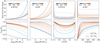Fig. 12. Top row: size of the gap after 2.5 Gyr of evolution as a function of the impact parameters (subhalo mass, angle θ, and amplitude of the relative velocity w). Bottom row: density contrast as a function of the same parameters. The two panels on the left show the discrete variation of the curves, varying the velocity amplitude w or collision angle θ. The two panels on the right show two sets of lines, solid for a subhalo of mass 107 M⊙ and dashed for 108 M⊙.

Because the size of a gap varies depending on its orbital phase, we confirmed that the dependences shown in Fig. 12 are robust. We found them to be identical, except for an overall scaling of the amplitude that depends on the phase. Because it is possible to establish the phase of a gap observationally (after assuming a suitable Galactic potential and integrating the orbit of the stream in which it is embedded), this implies that the trends observed here can be used to infer several of the characteristic properties of the encounter. The density contrast, meanwhile, does not vary along the orbit (because the density variations along the orbit for the gap are identical to those for the unperturbed stream). However, in the bottom panels of Fig. 12, we have taken the late times limit of the density contrast given by Eq. (34).

We showed in Eq. (8b) that the size of the gap at any point in time strongly depends on its initial magnitude (i.e. ∝r_s/cos θ), implying a dependence on the subhalo mass through the r_s parameter (with r_s ∝ M^2/5), as shown in Appendix B. This simple relation explains the curves in the top panels of Fig. 12 well, which show that the gap size depends strongly on the mass of the subhalo (two leftmost panels), with relatively little dependence on w and sin θ, except for extreme values of these parameters (two rightmost panels). For example, when the subhalo moves along the stream (i.e. when cos θ → 0), the size of the gap is clearly not well defined. In this case, the impulse approximation breaks down as the subhalo and stream interact for a long time, and perhaps more importantly, the interaction affects a large part of the stream. Moreover, for very low values of w, the impulse approximation is no longer valid. Low relative velocities and extreme alignment must be rare because they only occur when the stream and subhalo move at a similar velocity and in the same direction. In summary, the top panels of Fig. 12 suggest that given a gap size, it is possible to infer the mass of the subhalo that perturbed it with some confidence for most values of w and θ.

With the knowledge of the mass, the density contrast could be used to infer some plausible encounter geometries. To understand the factors driving the density contrast, we used Eq. (34), which depends on the ratio of det|σ_Θ0| for the stream and the gap. Although general analytic expressions can be obtained, they are somewhat cumbersome. Under the assumption that the velocity kick is small (compared to the characteristic orbital velocity of the subhalo) and that the covariance matrix of the stream at the time of the encounter is diagonal in Cartesian coordinates, we find (see Appendix C for full details)

$$\begin{array}{c}\hfill \delta {\rho }_{\mathrm{str}}^{\mathrm{gap}}\propto 1-\frac{\mathit{GM}}{r_s^{2}w}f(\theta ,\alpha ,{\mathbb{C}}_{{\mathit{x},\mathit{x}}_0}^{\mathrm{str}},{\mathbb{C}}_{{\mathit{v},\mathit{v}}_0}^{\mathrm{str}},vfg{\mathit{x}}_0,{\mathit{v}}_0),\end{array}$$(35)

where $f(\theta ,\alpha ,{\mathbb{C}}_{{\mathit{x},\mathit{x}}_0}^{\mathrm{str}},{\mathbb{C}}_{{\mathit{v},\mathit{v}}_0}^{\mathrm{str}},{\mathit{x}}_0,{\mathit{v}}_0)$ is a function that depends on the angles characterising the encounter, the location of the encounter (x₀, v₀), and the configuration and velocity covariance matrices of the unperturbed stream at the time of the impact (see also Eq. (C.16)). This relation implies that the density contrast becomes shallower with increasing w, as is shown in Fig. 12. On the other hand, more massive subhalos create gaps with lower densities. Because of the different dependence of the gap size (top panel) and of the density contrast with the characteristic parameters of the encounter, (M, w, sin θ), this means that it is possible to break some of the degeneracies present using these two observable quantities, provided the time since the collision can be established (which is necessary for making use of the constraints provided by gap size).

Another time-invariant combination of observables is plotted in Fig. 13. This figure shows the spatial size of the gap relative to the separation in velocity space, normalised by its initial value at t₀. Although the ratio of ΔX and ΔV does vary with the orbital phase of the gap or stream, this phase can be established through orbit integrations, as discussed earlier. The lines shown in Fig. 13 (measured at 2.5 Gyr) are for a gap that is near its apocentre. Evaluating the ratios ΔX/ΔV near the pericentre results in a similar figure, but where the y-axis is mirrored with respect to the line y = 0.

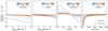Fig. 13. Sensitivity of the (time-independent) ratio of the size of the gap to the separation in velocity to the same parameters as discussed in Fig. 12.

There are clear similarities between this ratio and the behaviour of the density contrast shown in the bottom row of Fig. 12, except for the third panel, which reveals a sensitivity for low w velocity on the angle of the encounter θ. Overall, this ratio therefore is a good discriminator for low w of sin θ.

In summary, (smallish) gaps ≲25 kpc mostly depend on the mass of the subhalo, while large gaps can either be due to a specific configuration (low relative velocity or angle of the encounter) or due to a large subhalo. Assuming the average encounter has a relative speed of w >  200 km s⁻¹, it appears that per orbit or stream, we can break the degeneracy of the interaction parameters using the density contrast as well. We verified that these conclusions (and dependences) are robust and independent of the orbital characteristics of the stream (e.g., different inclinations with respect to the Galactic plane), but they are only strictly valid if the age of the gap can be well constrained.

5. Discussion

Action-angle variables have previously been used to describe streams and their gaps (e.g., Helmi et al. 1999; Helmi & Gomez 2007; Bovy 2014; Sanders et al. 2016; Helmi & Koppelman 2016; Bovy et al. 2017). There is a trade-off to be made when using these variables: we may either make use of a numerical approach and obtain a (local) approximation for a generic potential (Binney 2012; Sanders & Binney 2015), or use a fully analytic approach and be restricted in the choice of the potential. In this work, we took the latter approach such that we can express the properties of the gaps in physical space directly as a function of the encounter parameters.

In contrast to the work of Erkal & Belokurov (2015a), who argued that gaps grow at late times as $\sqrt{t}$ (for circular orbits), we find that both in our numerical experiments as in the analytic model, gaps grow linearly with time independently of the type of orbit or shape of the gravitational potential. We therefore extended the findings of HK16, who considered a spherical potential, and also confirmed the results of Sanders et al. (2016).

Sanders et al. (2016) have found that the density contrast of a gap approaches a constant value at late times. Our fully analytical model allowed us to verify their conclusion, and we were also able to show why this happens and on what the constant value depends (e.g., Eqs. (34) and (35)). Sanders et al. (2016) also reported that gaps grow differently in the leading and trailing arm. Judging from the expressions derived in this work, there may be two reasons for the different growth rate: (i) a difference in the local (velocity) dispersions of the particles in either the leading or trailing arm, as was already noted by Sanders et al. (2016), or (ii) the orbits of the leading and trailing stream have slightly different characteristic parameters (they are slightly offset in energy), and these affect the growth rate of gaps as well as the decline in their density.

Erkal & Belokurov (2015b) argued that a degeneracy exists in the gap parameters with mass and velocity. The reported degeneracy of (M, w)→(λM, λw) only exists if the scale radius r_s of the subhalo is kept fixed, but its mass is not. For example, the size of a gap depends on r_s, while the density contrast depends on $M/r_s^2$. Since a non-linear relation between r_s and M is known to exist for subhalos in cosmological simulations (r_s ∼ M^2/5, Neto et al. 2007; Springel et al. 2008), we must conclude that the above degeneracy does not exist for subhalos in CDM. A different mass-size scaling relation, for example for subhalos in other cosmologies or for other objects such as globular clusters and giant molecular clouds, will most likely also break the degeneracy unless the size is independent of the mass.

The model we presented successfully describes gaps in streams in axisymmetric potentials. However, it builds on several key assumptions that we list below.

The time of the collision or age of the gap. Although this information is in principle encoded in the size of the gap, we have generally explored its properties at a fixed time. Keeping it open will add one more parameter to optimise. A rough estimate of the formation time could be obtained by integrating the two sides of the gap backwards in time and determine when they meet. We recall, on the other hand, that if we may assume that the encounter occurred sufficiently long ago, the density contrast is independent of time, and some of the encounter parameters can be constrained.

The potential of the host galaxy. Changes in the host potential will change the central orbit of the gap and thus the size and density evolution. However, we note that the explicit time dependence of both the size and density of the gap will not change with (small) variations in the potential.

Knowledge of the pristine stream conditions before the interaction. In principle, it should be possible to derive the full 6D properties of the stream at the time of the collision from observing the full stream morphology and knowing the age of the gap.

The properties of the subhalo, here assumed to be well described by a Plummer sphere. This choice was made because of its simple mathematical expression, for which there is an analytic solution to the integral of the impulse approximation used to compute the velocity kicks. However, it is possible to compute this integral numerically for other profiles (e.g., Sanders et al. 2016).

We showed that some of the previously reported degeneracies in the space of parameters describing the encounter can be broken by making plausible assumptions about the stream-subhalo configuration. A natural next step would be to consider probability distributions for the encounter parameters, much like, for example, Erkal et al. (2016). Our model can then be used to quickly explore the parameter space as it can constrain the most likely encounter parameters given observation of a gap.

Finally, we discuss the possibility that gaps might be created by interactions with globular clusters and giant molecular clouds (GMCs). As long as they are massive and compact enough, GMCs can have a similar effect on cold streams as dark matter subhalos (Amorisco & Gómez 2016). Streams that orbit near the disc and thus have a high chance of encountering a GMC, are therefore not ideal as probes for dark matter substructures (such as Pal-5, see Banik & Bovy 2018). Because the orbits of GMCs and globular clusters are sufficiently well known, we can constrain the possible range of interaction parameters for these objects much better and rule them out as possible perturbers (e.g., Bonaca et al. 2019b and Banik et al. 2021).

To place this in the context of the equations derived in Sect. 4: The size of the gap is sensitive to the size (∼r_s) of the object. On the other hand, the density contrast depends on the ratio of the mass and scale radius ($\sim M/r_s^2$) and thus effectively is more sensitive to the density (or rather a surface density) of the perturber. Objects that pack more mass inside the same scale radius create larger gaps in terms of the density contrast. Globular clusters and GMCs, both of which are compact systems, will create different combinations of the gap size and density contrast than the typical dark matter subhalo. Gaps created by these compact objects are relatively small in size but large in density contrast.

6. Conclusions

We have successfully extended the model of the evolution of gaps in spherical potentials, presented in HK16, to describe gaps in streams orbiting in axisymmetric Stäckel potentials. The model accurately predicts the evolution of both the size of the gap and its central density. The model is unique in that it is fully analytic, meaning that we can directly relate the stream-subhalo interaction parameters to the properties of the resulting gaps. In doing so, it provides some interesting insights into the evolution of gaps in streams.

We find that the sizes of the gaps in axisymmetric potentials grow linearly in time and that this dependence is independent of the shape of the Galactic potential. On the other hand, the density declines in time as t⁻ⁿ , where n denotes the number of independent frequencies characterising its orbit. The growth of the size and density of a gap depend on the subhalo properties (mass and scale radius), the properties of the stream at the time of the impact (velocity and positional differences of the particles), and on the central orbit of the gap.

We have shown that the size of the gap is correlated with the portion of the stream most affected by the subhalo flyby (the value y_max in the impulse approximation). The density contrast of the gap, on the other hand, is more correlated with the amplitude of the interaction (Δv^max). These different correlations are in the end what drives the ability to break the degeneracy of the encounter parameters. For example, for a given gap age, small gaps (<25 kpc) are highly dependent on the size of the subhalo, while a large gap can be caused by a large subhalo or by an alignment of the orbit of the stream and subhalo. These results are encouraging and appear to be useful to constrain the properties of a population of dark subhalos if present in the halo of the Milky Way.

Acknowledgments

We gratefully acknowledge financial support from a VICI grant and a Spinoza Prize from the Netherlands Organisation for Scientific Research (NWO) and HHK is grateful for the support from the Martin A. and Helen Chooljian Membership at the Institute for Advanced Study. We thank Tim de Zeeuw and Denis Erkal for their comments on an early version of this manuscript and Hans Buist for modifications made to the code used here. For the analysis, the following software packages have been used: vaex (Breddels & Veljanoski 2018), numpy (Van Der Walt et al. 2011), matplotlib (Hunter 2007), jupyter notebooks (Kluyver et al. 2016), f2py (Peterson 2009), and pyGadgetReader (Thompson 2014).

References

Appendix A: Full 3D impulse of the covariance matrix

In this section we derive the change in covariance matrix when the full 3D morphology of the stream is taken into account. Similar to the 1D case, see Sect. 2.5, we assume that the change in velocity is a linear function of the spatial coordinates, meaning that the denominator of the kicks $(w((r_s^2+r^2)w^2-(\mathit{x}\cdot \mathit{w}{)}^2))\approx r_s^2{w}^3$. This approximation is in general true for the small volumes in which we measure the density, typically ≪1 kpc. This assumption allows us to rewrite Eqs. (7) to

$$\begin{array}{c}\hfill \mathrm{\Delta }{v}_i(\mathit{x})=-2GM\frac{w^2{x}_i-w_i(\mathit{x}·\mathit{w})}{r_s^2{w}^3},\end{array}$$(A.1)

where the subscript i = x, y, z.

In a similar procedure as for the 1D approximation, we can now compute the covariance terms. The velocity-position terms in the most general form are

$$\begin{array}{c}\hfill C(v_i+\mathrm{\Delta }{v}_i,x_j)=C(v_i,x_j)+\frac{1}{n}{\displaystyle \sum \mathrm{\Delta }}{v}_i(x_j-{\overline{x}}_j)\end{array}$$(A.2)

with

$$\begin{array}{c}\hfill \frac{1}{n}{\displaystyle \sum }\mathrm{\Delta }{v}_i(x_j-{\overline{x}}_j)=-\frac{2GM}{r_s^2{w}^3}[w^{2}C(x_i,x_j)-{\displaystyle \sum _{k=x,y,z}}{w}_i{w}_{k}C(x_k,x_j)].\end{array}$$(A.3)

The velocity-velocity terms are slightly more cumbersome,

$$\begin{array}{c}\hfill C(v_i+\mathrm{\Delta }{v}_i,v_j+\mathrm{\Delta }{v}_j)=C(v_i,v_j)+\frac{1}{n}{\displaystyle \sum \mathrm{\Delta }}{v}_i(v_j-{\overline{v}}_j)+\frac{1}{n}{\displaystyle \sum }(v_i-{\overline{v}}_i)\mathrm{\Delta }{v}_j+\frac{1}{n}{\displaystyle \sum \mathrm{\Delta }}{v}_i\mathrm{\Delta }{v}_j,\end{array}$$(A.4)

where

$$\begin{array}{c}\hfill \frac{1}{n}{\displaystyle \sum }\mathrm{\Delta }{v}_i(v_j-{\overline{v}}_j)=-\frac{2GM}{r_s^2{w}^3}[w^{2}C(x_i,v_j)-{\displaystyle \sum _{k=x,y,z}}{w}_i{w}_{k}C(x_k,v_j)].\end{array}$$(A.5)

The last term in Eq. (A.4) is

$$\begin{array}{cc}\hfill \frac{1}{n}{\displaystyle \sum }\mathrm{\Delta }{v}_i\mathrm{\Delta }{v}_j& =(\frac{2GM}{r_s^2{w}^3}{)}^2[w^{4}C(x_i,x_j)-{\displaystyle \sum _{k=x,y,z}}(w^2{w}_k[w_{j}C(x_i,x_k)+w_{i}C(x_j,x_k)]-w_i{w}_j{w}_k^{2}C(x_k,x_k))\hfill \\ \hfill & +w_i{w}_j(2w_x{w}_{y}C(x,y)+2w_x{w}_{z}C(x,z)+2w_y{w}_{z}C(y,z))].\hfill \end{array}$$(A.6)

These expressions take a much simpler form when the initial covariance matrix Σ_ϖ, 0 (e.g., Eq. (19)) is diagonal. In this case, Eq. (A.4) simplifies to

$$\begin{array}{c}\hfill \frac{1}{n}{\displaystyle \sum }\mathrm{\Delta }{v}_i(x_j-{\overline{x}}_j)=-ϵ\frac{w}{r_s}C(x_j,x_j)[{\delta }_{\mathit{ij}}-\frac{w_i{w}_j}{w^2}],\end{array}$$(A.7)

where

$$\begin{array}{c}\hfill ϵ=\frac{2GM}{r_s{w}^2}\end{array}$$(A.8)

is a unit less parameter and δ_ij is the Kronecker delta. Equation (A.5) simply vanishes because it only features off-diagonal terms, and Eq. (A.6) reduces to

$$\begin{array}{c}\hfill \frac{1}{n}{\displaystyle \sum }\mathrm{\Delta }{v}_i\mathrm{\Delta }{v}_j={ϵ}^2{w}^2[\frac{C(x_i,x_j)}{r_s^2}-\frac{w_i{w}_j}{w^2{r}_s^2}[C(x_i,x_i)+C(x_j,x_j)]+{\displaystyle \sum _{k=x,y,z}}(\frac{w_i{w}_j{w}_k^2}{w^4}\frac{C(x_k,x_k)}{r_s^2})].\end{array}$$(A.9)

In Appendix C we return to these simplified expressions. It is convenient to express Eqs. (A.7) and (A.9) in terms of ϵ and another parameter (Δ_ij and D_ij, respectively) that carries all other terms, such that in this specific case we can write

$$\begin{array}{c}\hfill \frac{1}{n}{\displaystyle \sum }\mathrm{\Delta }{v}_i(x_j-{\overline{x}}_j)=-ϵ{\mathrm{\Delta }}_{\mathit{ij}},\end{array}$$(A.10)

and

$$\begin{array}{c}\hfill \frac{1}{n}{\displaystyle \sum }\mathrm{\Delta }{v}_i\mathrm{\Delta }{v}_j={ϵ}^2{D}_{\mathit{ij}}.\end{array}$$(A.11)

Appendix B: Subhalo scaling relations

For the scaling of the subhalos scale radius r_s with mass M, we have used several scaling relations that we list below. To obtain the scaling, we first related the subhalo mass M with the maximum circular velocity V_max = V_c(r_max). Springel et al. (2008; see their Fig. 27) reported

$$\begin{array}{c}\hfill V_{\max }=(\frac{M}{3.37·{10}^7{M}_{\odot }}{)}^{1/3.49}·10{\mathrm{km}\mathrm{s}}^{-1},\end{array}$$(B.1)

which is an empirical scaling relation based on the subhalos down to the mass range of ≲10⁵ M_⊙, identified in the Aquarius simulations. Next, r_max is related to V_max using Eqs. (6)–(9) from Springel et al.,

$$\begin{array}{c}\hfill r_{\max }=V_{\max }[\frac{{\delta }_c{H}_0^2}{14.426}{]}^{-\frac{1}{2}}·0.62,\end{array}$$(B.2)

where the factor 0.62 was added based on the comment in the caption of Fig. 26 of Springel et al. (2008, see also below), and we assumed H₀ = 73 km s⁻¹ Mpc⁻¹. The final missing piece is δ_c, which is related to the concentration parameter c by

$$\begin{array}{c}\hfill {\delta }_c=\frac{200}{3}{c}^3(log(1+c)-\frac{c}{1+c}{)}^{-1}.\end{array}$$(B.3)

Typically, c is related to the subhalo mass M, motivated by Springel et al. (2008). We relate the two using an empirical scaling relation found by Neto et al. (2007) for relaxed halos

$$\begin{array}{c}\hfill c=5.26(\frac{M}{h·{10}^{14}}{)}^{-0.10},\end{array}$$(B.4)

where h = H₀/(100 km s⁻¹). We note that Springel et al. (2008) reported that the resulting scaling relation of V_max ∼ r_max is lower than the relation found from extrapolating the results of Neto et al. (which is not calibrated for subhalos in the low-mass range that we consider here). The offset is 0.62, therefore we added this factor in Eq. (B.2).

With the equations above we can relate the subhalo mass M to V_max and a corresponding r_max. The scale radius r_s, NFW is related to r_max simply as

$$\begin{array}{c}\hfill r_{\max }=2.163·r_{s,\mathrm{NFW}},\end{array}$$(B.5)

which is found numerically from calculating where V_c(r_max) = V_max (but see Eq. (11) of Diemand et al. 2007, where we originally found the relation).

Finally, in this main text we used a Plummer profile to describe the subhalos, rather than a Navarro et al. (1997, NFW) profile. Therefore we relate the scale radii of the two profiles by equation the acceleration at r_max

$$\begin{array}{c}\hfill a_{\mathrm{NFW}}(r_{\max })=a_{\mathrm{Plummer}}(r_{\max })=-\frac{\mathit{GM}}{{(r_{\max }^2+r_s^2)}^{3/2}}·r_{\max }.\end{array}$$(B.6)

The scale radius of the Plummer, r_s, can be found by solving the equation above, which then is a function of M only. Finally, by fitting the scaling relation numerically, we find that the scale radius depends on mass as r_s ∝ M^0.397 ∼ M^2/5.

Appendix C: Computing the density contrast at late times

As described in the main paper, the density contrast at late times takes the form (see Eq. (34))

$$\begin{array}{c}\hfill \delta {\rho }_{\mathrm{str}}^{\mathrm{gap}}=\sqrt{\frac{det{|{\sigma }_{{\mathrm{\Theta }}_0}|}_{\mathrm{str}}}{det{|{\sigma }_{{\mathrm{\Theta }}_0}|}_{\mathrm{gap}}}}.\end{array}$$(C.1)

To be able to establish its dependence on the characteristic parameters of the encounter, we need to determine the form of the determinant of the matrix σ_Θ0. This is the upper left 3 × 3 submatrix of σ_ω, 0 that is described in Sect. 2.5. This matrix, following the notation of Sect. 2.4, takes the form

$$\begin{array}{c}\hfill {\sigma }_{\omega ,0}={{\mathcal{M}}_0^{-1}}^{†}{\sigma }_{\varpi ,0}{\mathcal{M}}_0^{-1},\end{array}$$(C.2)

where ℳ₀ is given by Eq. (12), namely ${\mathcal{M}}_0={\mathcal{M}}_0^{\mathrm{AA}\leftarrow \mathrm{st}}{\mathcal{M}}_0^{\mathrm{st}\leftarrow \mathrm{cyl}}{\mathcal{M}}_0^{\mathrm{cyl}\leftarrow \mathrm{xyz}}$, and thus represents the coordinate transformations from Cartesian to action-angle variables. For example, the matrix that accounts for the transformation from Stäckel coordinates to action angles, ${\mathcal{M}}_0^{\mathrm{AA}\leftarrow \mathrm{st}}$, contains the derivatives of the characteristic function and its general form is given in Eq. (A2) of HW99. In Eq. (C.2), ${\sigma }_{\varpi }^{-1}={\mathrm{\Sigma }}_{\varpi }$ is the inverse of the 6 × 6 covariance matrix in Cartesian coordinates. Therefore σ_Θ0 for the stream depends on location as well as on the initial properties of the stream, and similarly for the gap.

The matrix σ_ϖ, 0 is of the form

$$\begin{array}{c}\hfill {\sigma }_{\varpi ,0}=\left(\begin{array}{cc}{\sigma }_{\mathit{x},0}& {\sigma }_{\mathit{xv},0}\\ {\sigma }_{\mathit{x}v,0}^{†}& {\sigma }_{\mathit{v},0}\end{array}\right),\end{array}$$(C.3)

and because we may express as

$$\begin{array}{c}\hfill {\mathcal{M}}_0^{-1}=\left(\begin{array}{cc}A& B\\ C& D\end{array}\right),\end{array}$$(C.4)

this means that

$$\begin{array}{c}\hfill {\sigma }_{{\mathrm{\Theta }}_0}=A^{†}{\sigma }_{\mathit{x},0}A+C^{†}{\sigma }_{\mathit{xv},0}^{†}A+A^{†}{\sigma }_{\mathit{xv},0}C+C^{†}{\sigma }_{\mathit{v},0}^{†}C.\end{array}$$(C.5)

Using matrix inversions, if

$$\begin{array}{c}\hfill {\mathcal{M}}_0=\left(\begin{array}{cc}{t}_1& t_2\\ t_3& t_4\end{array}\right),\end{array}$$(C.6)

and t₄ is invertible, then

$$\begin{array}{c}\hfill A={(t_1-t_2{t}_4^{-1}{t}_3)}^{-1},\mathrm{and}C=-t_4^{-1}{t}_{3}A=T_{43}A,\end{array}$$(C.7)

where we recall that A and T₄₃ represent coordinate transformations and therefore only depend on location. These matrices were set to be identical for the gap and the stream in Eq. (C.1), which significantly simplifies subsequent computations. When we now replace in Eq. (C.5), this results in

$$\begin{array}{c}\hfill det|{\sigma }_{{\mathrm{\Theta }}_0}{|=(detA)}^{2}det({\sigma }_{\mathit{x},0}+T_{43}^{†}{\sigma }_{\mathit{xv},0}^{†}+{\sigma }_{\mathit{xv},0}{T}_{43}+T_{43}^{†}{\sigma }_{\mathit{v},0}^{†}{T}_{43}).\end{array}$$(C.8)

The expression for det|σ_Θ0|_str using the above equation has been worked out in detail by HW99 for a stream generated from an initially isotropic Gaussian distribution in configuration and velocity space and for a preferred location along the orbit, namely the apocentre. The explicit expressions in the case of an axisymmetric system (the last equation in their Appendix B), and for a system described with Stäckel coordinates (Eq. C13 in their Appendix C) are presented in HW99.

We now proceed to determine the form of the submatrices of σ_ϖ, 0 given in Eq. (C.3) and needed in Eq. (C.8). For the stream we assumed no initial correlations between positions and velocities in the stream (i.e. a diagonal covariance matrix Σ_ϖ, 0), which means that the submatrix ${\sigma }_{\mathit{xv},0}^{\mathrm{str}}=0$ and that ${\sigma }_{\mathit{x},0}^{\mathrm{str}}={[{\mathbb{C}}_{{\mathit{x},\mathit{x}}_0}^{\mathrm{str}}]}^{-1}$ and ${\sigma }_{\mathit{v},0}^{\mathrm{str}}={[{\mathbb{C}}_{{\mathit{v},\mathit{v}}_0}^{\mathrm{str}}]}^{-1}$ according to Eq. (19). For the gap, we may express

$$\begin{array}{c}\hfill {\mathbb{C}}_{{\mathit{v},\mathit{v}}_0}^{\mathrm{gap}}={\mathbb{C}}_{{\mathit{v},\mathit{v}}_0}^{\mathrm{str}}+{ϵ}^2\mathbf{D},\end{array}$$(C.9)

where the elements of D are given by D_ij, see Eq. (A.11). Furthermore,

$$\begin{array}{c}\hfill {\mathbb{C}}_{{\mathit{x},\mathit{v}}_0}^{\mathrm{gap}}=-ϵ\mathrm{\Delta },\end{array}$$(C.10)

where the elements of Δ are given by Δ_ij, see Eq. (A.10).

To compute the submatrices ${\sigma }_{\mathit{x},0}^{\mathrm{gap}}$, ${\sigma }_{\mathit{xv},0}^{\mathrm{gap}}$ , and ${\sigma }_{\mathit{v},0}^{\mathrm{gap}}$, in Eq. (C.8), we use that ${\sigma }_{\varpi ,0}^{\mathrm{gap}}={{\mathrm{\Sigma }}_{\varpi ,0}^{\mathrm{gap}}}^{-1}$, which is given by Eq. (20). The inverse of this block matrix can be computed explicitly, provided the matrix $W={\mathbb{C}}_{{\mathit{v},\mathit{v}}_0}^{\mathrm{gap}}-{{\mathbb{C}}_{{\mathit{x},\mathit{v}}_0}^{\mathrm{gap}}}^{†}{[{\mathbb{C}}_{{\mathit{x},\mathit{x}}_0}^{\mathrm{gap}}]}^{-1}{\mathbb{C}}_{{\mathit{x},\mathit{v}}_0}^{\mathrm{gap}}$ is invertible. Using Eqs. (C.9) and (C.10), and to the lowest order in ϵ, we find that

$$\begin{array}{cc}& {\sigma }_{\mathit{v},0}^{\mathrm{gap}}=W^{-1}\approx {[{\mathbb{C}}_{{\mathit{v},\mathit{v}}_0}^{\mathrm{str}}]}^{-1}[\mathbf{I}-{ϵ}^2(\mathbf{D}-{\mathrm{\Delta }}^{†}{[{\mathbb{C}}_{{\mathit{x},\mathit{x}}_0}^{\mathrm{str}}]}^{-1}\mathrm{\Delta }){[{\mathbb{C}}_{{\mathit{v},\mathit{v}}_0}^{\mathrm{str}}]}^{-1}],\hfill \end{array}$$(C.11)

$$\begin{array}{cc}\hfill & {\sigma }_{\mathit{xv},0}^{\mathrm{gap}}=ϵ{[{\mathbb{C}}_{{\mathit{x},\mathit{x}}_0}^{\mathrm{str}}]}^{-1}\mathrm{\Delta }{[{\mathbb{C}}_{{\mathit{v},\mathit{v}}_0}^{\mathrm{str}}]}^{-1}\hfill \end{array}$$(C.12)

$$\begin{array}{cc}\hfill & {\sigma }_{\mathit{x},0}^{\mathrm{gap}}={[{\mathbb{C}}_{{\mathit{x},\mathit{x}}_0}^{\mathrm{str}}]}^{-1}+{ϵ}^2{[{\mathbb{C}}_{{\mathit{x},\mathit{x}}_0}^{\mathrm{str}}]}^{-1}\mathrm{\Delta }{[{\mathbb{C}}_{{\mathit{v},\mathit{v}}_0}^{\mathrm{str}}]}^{-1}{\mathrm{\Delta }}^{†}{[{\mathbb{C}}_{{\mathit{x},\mathit{x}}_0}^{\mathrm{str}}]}^{-1}.\hfill \end{array}$$(C.13)

We are now almost ready to compute the density contrast because

$$\begin{array}{c}\hfill det|{\sigma }_{{\mathrm{\Theta }}_0}{|}_{\mathrm{gap}}\sim {(detA)}^{2}det[{\sigma }_{\mathit{x},0}^{\mathrm{str}}+T_{43}^{†}{\sigma }_{\mathit{v},0}^{\mathrm{str}}{T}_{43}+ϵ(T_{43}^{†}{\sigma }_{\mathit{v},0}^{\mathrm{str}}{\mathrm{\Delta }}^{†}{\sigma }_{\mathit{x},0}^{\mathrm{str}}+{\sigma }_{\mathit{x},0}^{\mathrm{str}}\mathrm{\Delta }{\sigma }_{\mathit{v},0}^{\mathrm{str}}{T}_{43})]\sim det{|{\sigma }_{{\mathrm{\Theta }}_0}|}_{\mathrm{str}}det[\mathbf{I}+ϵ\mathbf{K}],\end{array}$$(C.14)

where the matrix K is

$$\begin{array}{c}\hfill \mathbf{K}=[T_{43}^{†}{\sigma }_{\mathit{v},0}^{\mathrm{str}}{\mathrm{\Delta }}^{†}{\sigma }_{\mathit{x},0}^{\mathrm{str}}+{\sigma }_{\mathit{x},0}^{\mathrm{str}}\mathrm{\Delta }{\sigma }_{\mathit{v},0}^{\mathrm{str}}{T}_{43}]{[{\sigma }_{\mathit{x},0}^{\mathrm{str}}+T_{43}^{†}{\sigma }_{\mathit{v},0}^{\mathrm{str}}{T}_{43}]}^{-1},\end{array}$$(C.15)

and it is therefore dependent on the initial properties of the stream (at the time of the encounter and through the σ matrices), the location of the encounter in phase-space (through the matrix T₄₃ introduced in Eq. (C.7)), and the characteristic parameters of the encounter (through the matrix Δ, whose elements can be described as $\frac{\mathit{w}}{r_s}$ times some function $g({\mathbb{C}}_{{\mathit{x},\mathit{x}}_0}^{\mathrm{s}\mathrm{t}\mathrm{r}},\alpha ,\theta )$, see Eqs. (A.7) and (A.10)). Because we may express det[I + ϵ K]∼1 + ϵ trK, the density contrast at late times becomes

$$\begin{array}{c}\hfill \delta {\rho }_{\mathrm{str}}^{\mathrm{gap}}\sim \sqrt{\frac{det{|{\sigma }_{{\mathrm{\Theta }}_0}|}_{\mathrm{str}}}{det{|{\sigma }_{{\mathrm{\Theta }}_0}|}_{\mathrm{gap}}}}\sim {(1+ϵ\mathrm{tr}\mathbf{K})}^{-1/2}\sim 1-\frac{ϵ}{2}\mathrm{tr}\mathbf{K}\sim 1-\frac{\mathit{GM}}{r_s^{2}w}f(\theta ,\alpha ,{\mathbb{C}}_{{\mathit{x},\mathit{x}}_0}^{\mathrm{str}},{\mathbb{C}}_{{\mathit{v},\mathit{v}}_0}^{\mathrm{str}},{\mathit{x}}_0,{\mathit{v}}_0),\end{array}$$(C.16)

where $f(\theta ,\alpha ,{\mathbb{C}}_{{\mathit{x},\mathit{x}}_0}^{\mathrm{str}},{\mathbb{C}}_{{\mathit{v},\mathit{v}}_0}^{\mathrm{str}},{\mathit{x}}_0,{\mathit{v}}_0)$ is a function that depends on the impact configuration and initial state of the stream.

All Tables

All Figures

	Fig. 1. Circular velocity in the plane of the disc of our Milky Way model. The Stäckel potential comprises a disc and a halo component and realistically describes the circular velocity of the Milky Way in the inner ∼20 kpc, as can be seen by comparing to the determinations by Eilers et al. (2019).
In the text

	Fig. 2. Schematic overview of the stream-subhalo interaction. Left: view seen from the top. Right: view seen along the line of sight (stream away from the observer).
In the text

Fig. 3. Orbit of the stream shown in galactocentric Cartesian coordinates, evolved for 10 Gyr forward in time in the Stäckel axisymmetric Milky Way-like potential. Top: orbit in coordinates aligned with the host galaxy (e.g., plane of the disc is z = 0). Bottom: coordinates aligned with the initial angular momentum vector of the orbit. The bottom right panel highlights the precession of the orbital plane, which is indicative of the non-spherical nature of the potential considered.

In the text

Fig. 4. Left: snapshot of a stream at the time of interaction with a subhalo. The stream is plotted with black dots, and the centre of mass of the subhalo is shown as a solid red circle. The velocity vector of the stream is marked with a black arrow and that of the subhalo with a red arrow. Right: both panels show the stream after 2 Gyr of evolution, in isolation in the top panel, and after the encounter with the subhalo in the bottom panel.

In the text

Fig. 5. Top panel: gaps growing in a stream orbiting an axisymmetric Stäckel Milky Way-like potential. The lines with different colours show the size of the gaps induced by subhalos of different sizes. The solid curves correspond to our analytic model, and the dashed curves to gaps measured in the N-body experiments. The straight dashed grey lines illustrate the linear growth rate of the gaps. Bottom panel: distance of the central orbit to the centre of the host potential.

In the text

	Fig. 6. Left: stream 1 Gyr after an interaction with a subhalo. The two red dots indicate the orbits that were used to measure the size of the gap, and the red arrow shows the distance on a straight line between the two dots. Right: same stream 3.6 Gyr after the encounter. At this point in time, the two orbits (red dots) are close to their maximum separation.
In the text

	Fig. 7. Density evolution of an unperturbed stream (in blue) and of a gap in a stream following the same orbit (in green). The dashed curves are the densities obtained from the corresponding N-body experiments. The agreement between the solid and dashed curves is excellent. The subhalo that is used to create the gap in the stream has a mass of 107 M⊙.
In the text

Fig. 8. Density contrast measured for a stream experiencing an encounter with subhalos of different mass and scale radius, see Table 1. The relative velocity of the impact is the same for all three interactions. The coloured solid lines show the density contrast according to our model, and the dashed lines are measured in the N-body experiments. The shaded areas indicate the Poisson error in the observed density. The subhalo of 108 M⊙ is shown in a different panel because of its slightly different set-up.

In the text

	Fig. 9. Similar to Fig. 5, but for three different configurations of the stream-subhalo interactions. The gaps of all configurations are created by the same subhalo of size 107 M⊙, but their relative velocity w and impact angles θ and α are different.
In the text

References

- Amorisco, N. C., Gómez, F. A., et al. 2016, MNRAS, 463, L17 [NASA ADS] [CrossRef] [Google Scholar]
- Banik, N., & Bovy, J. 2018, MNRAS, 484, 2009 [Google Scholar]
- Banik, N., Bovy, J., Bertone, G., Erkal, D., & de Boer, T. J. L. 2021, MNRAS, 502, 2364 [NASA ADS] [CrossRef] [Google Scholar]
- Batsleer, P., & Dejonghe, H. 1994, A&A, 287, 43 [NASA ADS] [Google Scholar]
- Belokurov, V., Zucker, D. B., Evans, N. W., et al. 2006, ApJ, 642, L137 [Google Scholar]
- Bernard, E. J., Ferguson, A. M. N., Schlafly, E. F., et al. 2016, MNRAS, 463, 1759 [NASA ADS] [CrossRef] [Google Scholar]
- Binney, J. 2012, MNRAS, 426, 1324 [Google Scholar]
- Binney, J., & Tremaine, S. 2008, Galactic Dynamics (Princeton University Press), 885 [CrossRef] [Google Scholar]
- Bode, P., Ostriker, J. P., & Turok, N. 2001, ApJ, 556, 93 [Google Scholar]
- Bonaca, A., Conroy, C., Price-Whelan, A. M., & Hogg, D. W. 2019a, ApJ, 881, L37 [NASA ADS] [CrossRef] [Google Scholar]
- Bonaca, A., Hogg, D. W., Price-Whelan, A. M., & Conroy, C. 2019b, ApJ, 880, 38 [NASA ADS] [CrossRef] [Google Scholar]
- Bonaca, A., Conroy, C., Hogg, D. W., et al. 2020, ApJ, 892, L37 [NASA ADS] [CrossRef] [Google Scholar]
- Bovy, J. 2014, ApJ, 795, 20 [NASA ADS] [CrossRef] [Google Scholar]
- Bovy, J., Erkal, D., & Sanders, J. L. 2017, MNRAS, 466, 628 [NASA ADS] [CrossRef] [Google Scholar]
- Bozek, B., Boylan-Kolchin, M., Horiuchi, S., et al. 2016, MNRAS, 459, 1489 [NASA ADS] [CrossRef] [Google Scholar]
- Breddels, M. A., & Veljanoski, J. 2018, A&A, 618, A13 [NASA ADS] [CrossRef] [EDP Sciences] [Google Scholar]
- Bullock, J. S., & Boylan-Kolchin, M. 2017, ARA&A, 55, 343 [NASA ADS] [CrossRef] [Google Scholar]
- Carlberg, R. G. 2013, ApJ, 775, 90 [NASA ADS] [CrossRef] [Google Scholar]
- Carlberg, R. G., & Grillmair, C. J. 2013, ApJ, 768, 171 [NASA ADS] [CrossRef] [Google Scholar]
- Dalal, N., & Kochanek, C. S. 2002, ApJ, 572, 25 [NASA ADS] [CrossRef] [Google Scholar]
- Davis, M., Efstathiou, G., Frenk, C. S., & White, S. D. M. 1985, ApJ, 292, 371 [NASA ADS] [CrossRef] [Google Scholar]
- De Boer, T. J. L., Belokurov, V., Koposov, S. E., et al. 2018, MNRAS, 477, 1893 [NASA ADS] [CrossRef] [Google Scholar]
- Dejonghe, H., & de Zeeuw, T. 1988, ApJ, 333, 90 [NASA ADS] [CrossRef] [Google Scholar]
- de Zeeuw, T. 1985, MNRAS, 216, 273 [NASA ADS] [CrossRef] [Google Scholar]
- Diemand, J., Kuhlen, M., & Madau, P. 2007, ApJ, 667, 859 [NASA ADS] [CrossRef] [Google Scholar]
- Diemand, J., Kuhlen, M., Madau, P., et al. 2008, Nature, 454, 735 [NASA ADS] [CrossRef] [PubMed] [Google Scholar]
- D’Onghia, E., Springel, V., Hernquist, L., & Keres, D. 2010, ApJ, 709, 1138 [NASA ADS] [CrossRef] [Google Scholar]
- Eilers, A.-C., Hogg, D. W., Rix, H.-W., & Ness, M. K. 2019, ApJ, 871, 120 [NASA ADS] [CrossRef] [Google Scholar]
- Erkal, D., & Belokurov, V. 2015a, MNRAS, 450, 1136 [Google Scholar]
- Erkal, D., & Belokurov, V. 2015b, MNRAS, 454, 3542 [NASA ADS] [CrossRef] [Google Scholar]
- Erkal, D., Belokurov, V., Bovy, J., & Sanders, J. L. 2016, MNRAS, 463, 102 [NASA ADS] [CrossRef] [Google Scholar]
- Erkal, D., Koposov, S. E., & Belokurov, V. 2017, MNRAS, 470, 60 [NASA ADS] [CrossRef] [Google Scholar]
- Famaey, B., & Dejonghe, H. 2003, MNRAS, 340, 752 [Google Scholar]
- Gaia Collaboration (Prusti, T., et al.) 2016, A&A, 595, A1 [NASA ADS] [CrossRef] [EDP Sciences] [Google Scholar]
- Gaia Collaboration (Brown, A. G. A., et al.) 2018, A&A, 616, A1 [NASA ADS] [CrossRef] [EDP Sciences] [Google Scholar]
- Goldstein, H., Poole, C., Safko, J., & Addison, S. R. 2002, Classical Mechanics, 3rd edn. (New York: Addison-Wesley), 638 [Google Scholar]
- Grillmair, C. J., & Dionatos, O. 2006, ApJ, 643, L17 [Google Scholar]
- Harris, W. E. 1996, AJ, 112, 1487 [NASA ADS] [CrossRef] [Google Scholar]
- Helmi, A., & Gomez, F. 2007, ArXiv e-prints [arxiv:0710.0514] [Google Scholar]
- Helmi, A., & Koppelman, H. H. 2016, ApJ, 828, L10 [NASA ADS] [CrossRef] [Google Scholar]
- Helmi, A., & White, S. D. M. 1999, MNRAS, 307, 495 [Google Scholar]
- Helmi, A., White, S. D. M., De Zeeuw, P. T., et al. 1999, Nature, 402, 53 [NASA ADS] [CrossRef] [Google Scholar]
- Hsueh, J. W., Enzi, W., Vegetti, S., et al. 2020, MNRAS, 492, 3047 [CrossRef] [Google Scholar]
- Hu, W., Barkana, R., & Gruzinov, A. 2000, Phys. Rev. Lett., 85, 1158 [Google Scholar]
- Hui, L., Ostriker, J. P., Tremaine, S., & Witten, E. 2017, Phys. Rev., D, 95, 043541 [NASA ADS] [Google Scholar]
- Hunter, J. D. 2007, Comput. Sci. Eng., 9, 90 [NASA ADS] [CrossRef] [Google Scholar]
- Ibata, R. A., Lewis, G. F., Irwin, M. J., & Quinn, T. 2002, MNRAS, 332, 915 [Google Scholar]
- Ibata, R. A., Malhan, K., & Martin, N. F. 2019, ApJ, 872, 152 [Google Scholar]
- Ibata, R., Thomas, G., Famaey, B., et al. 2020, ApJ, 891, 161 [Google Scholar]
- Johnston, K. V., Spergel, D. N., & Haydn, C. 2002, ApJ, 570, 656 [NASA ADS] [CrossRef] [Google Scholar]
- Kluyver, T., Ragan-Kelley, B., Pérez, F., et al. 2016, Jupyter Notebooks-a Publishing Format for Reproducible Computational Workflows (IOS Press) [Google Scholar]
- Klypin, A., Kravtsov, A. V., Valenzuela, O., & Prada, F. 1999, ApJ, 522, 82 [Google Scholar]
- Li, T. S., Koposov, S. E., Erkal, D., et al. 2021, ApJ, 911, 149 [CrossRef] [Google Scholar]
- Malhan, K., Ibata, R. A., & Martin, N. F. 2018, MNRAS, 481, 3442 [Google Scholar]
- Moore, B., Ghigna, S., Governato, F., et al. 1999, ApJ, 524, L19 [Google Scholar]
- Navarro, J. F., Frenk, C. S., & White, S. D. M. 1997, ApJ, 490, 493 [NASA ADS] [CrossRef] [Google Scholar]
- Neto, A. F., Gao, L., Bett, P., et al. 2007, MNRAS, 381, 1450 [NASA ADS] [CrossRef] [Google Scholar]
- Odenkirchen, M., Grebel, E. K., Rockosi, C. M., et al. 2001, ApJ, 548, L165 [Google Scholar]
- Pearson, S., Price-Whelan, A. M., & Johnston, K. V. 2017, Nat. Astron., 1, 633 [NASA ADS] [CrossRef] [Google Scholar]
- Peterson, P. 2009, Int. J. Comput. Sci. Eng., 4, 296 [Google Scholar]
- Price-Whelan, A. M., & Bonaca, A. 2018, ApJ, 863, L20 [CrossRef] [Google Scholar]
- Reino, S., Rossi, E. M., Sanderson, R. E., et al. 2021, MNRAS, 502, 4170 [NASA ADS] [CrossRef] [Google Scholar]
- Ritondale, E., Vegetti, S., Despali, G., et al. 2019, MNRAS, 485, 2179 [CrossRef] [Google Scholar]
- Sanders, J. L., & Binney, J. 2015, MNRAS, 447, 2479 [NASA ADS] [CrossRef] [Google Scholar]
- Sanders, J. L., Bovy, J., & Erkal, D. 2016, MNRAS, 457, 3817 [NASA ADS] [CrossRef] [Google Scholar]
- Sanderson, R. E., Vera-Ciro, C., Helmi, A., & Heit, J. 2016, ArXiv e-prints [arXiv:1608.05624] [Google Scholar]
- Sawala, T., Pihajoki, P., Johansson, P. H., et al. 2017, MNRAS, 467, 4383 [NASA ADS] [CrossRef] [Google Scholar]
- Shipp, N., Drlica-Wagner, A., Balbinot, E., et al. 2018, ApJ, 862, 114 [Google Scholar]
- Shipp, N., Li, T. S., Pace, A. B., et al. 2019, ApJ, 885, 3 [NASA ADS] [CrossRef] [Google Scholar]
- Spergel, D. N., & Steinhardt, P. J. 2000, Phys. Rev. Lett., 84, 1 [NASA ADS] [CrossRef] [PubMed] [Google Scholar]
- Springel, V. 2005, MNRAS, 364, 1105 [Google Scholar]
- Springel, V., Wang, J., Vogelsberger, M., et al. 2008, MNRAS, 391, 1685 [NASA ADS] [CrossRef] [Google Scholar]
- Thomas, G., Ibata, R., Famaey, B., Martin, N., & Lewis, G. 2016, MNRAS, 460, 2711 [NASA ADS] [CrossRef] [Google Scholar]
- Thompson, R. 2014, Astrophysics Source Code Library [record ascl:1411.001] [Google Scholar]
- Van Der Walt, S., Colbert, S. C., & Varoquaux, G. 2011, Comput. Sci. Eng., 13, 22 [Google Scholar]
- Vegetti, S., Koopmans, L. V. E., Bolton, A., Treu, T., & Gavazzi, R. 2010, MNRAS, 408, 1969 [NASA ADS] [CrossRef] [Google Scholar]
- Vegetti, S., Lagattuta, D. J., McKean, J. P., et al. 2012, Nature, 481, 341 [NASA ADS] [CrossRef] [Google Scholar]
- Vogelsberger, M., White, S. D. M., Helmi, A., & Springel, V. 2008, MNRAS, 385, 236 [NASA ADS] [CrossRef] [Google Scholar]
- Vogelsberger, M., Zavala, J., Cyr-Racine, F.-Y., et al. 2016, MNRAS, 460, 1399 [NASA ADS] [CrossRef] [Google Scholar]
- Yoon, J. H., Johnston, K. V., & Hogg, D. W. 2011, ApJ, 731, 58 [NASA ADS] [CrossRef] [Google Scholar]
- Zhu, Q., Marinacci, F., Maji, M., et al. 2016, MNRAS, 458, 1559 [Google Scholar]