| Issue |
A&A
Volume 649, May 2021
|
|
|---|---|---|
| Article Number | A98 | |
| Number of page(s) | 8 | |
| Section | Planets and planetary systems | |
| DOI | https://doi.org/10.1051/0004-6361/202039796 | |
| Published online | 19 May 2021 | |
Asteroid absolute magnitudes and phase curve parameters from Gaia photometry★
1
Nordic Optical Telescope (NOT),
Apartado 474,
38700
Santa Cruz de La Palma,
Spain
2
Department of Physics, University of Helsinki,
Gustaf Hällströmin katu 2, PO Box 64,
00014
U. Helsinki, Finland
e-mail: This email address is being protected from spambots. You need JavaScript enabled to view it.
3
Finnish Geospatial Research Institute FGI,
Geodeetinrinne 2,
02430
Masala, Finland
4
INAF, Osservatorio Astrofisico di Torino,
Via Osservatorio 20,
10025
Pino Torinese, Italy
5
Yunnan Observatories, CAS,
Kunming
650216, PR China
6
School of Astronomy and Space science, University of Chinese Academy of Sciences,
Beijing
100049,
PR China
Received:
29
October
2020
Accepted:
17
March
2021
Abstract
Aims. We perform light curve inversion for 491 asteroids to retrieve phase curve parameters, rotation periods, pole longitudes and latitudes, and convex and triaxial ellipsoid shapes by using the sparse photometric observations from Gaia Data Release 2 and the dense ground-based observations from the DAMIT database. We develop a method for the derivation of reference absolute magnitudes and phase curves from the Gaia data, allowing for comparative studies involving hundreds of asteroids.
Methods. For both general convex shapes and ellipsoid shapes, we computed least-squares solutions using either the Levenberg-Marquardt optimization algorithm or the Nelder-Mead downhill simplex method. Virtual observations were generated by adding Gaussian random errors to the observations, and, later on, a Markov chain Monte Carlo method was applied to sample the spin, shape, and scattering parameters. Absolute magnitude and phase curve retrieval was developed for the reference geometry of equatorial illumination and observations based on model magnitudes averaged over rotational phase.
Results. The derived photometric slope values showed wide variations within each assumed Tholen class. The computed Gaia G-band absolute magnitudes matched notably well with the V-band absolute magnitudes retrieved from the Jet Propulsion Laboratory Small-Body Database. Finally, the reference phase curves were well fitted with the H, G1, G2 phase function. The resulting G1, G2 distribution differed, in an intriguing way, from the G1, G2 distribution that is based on the phase curves corresponding to light curve brightness maxima.
Key words: minor planets, asteroids: general / methods: numerical / techniques: photometric
Phase curve data are only available at the CDS via anonymous ftp to cdsarc.u-strasbg.fr (130.79.128.5) or via http://cdsarc.u-strasbg.fr/viz-bin/cat/J/A+A/649/A98
© ESO 2021
1 Introduction
Asteroids are rocky, irregularly shaped airless bodies that have remained mostly the same for the past 4.5 billion years, providing us with information on the origin, evolution, and current state of the Solar System and its entire small-body population. Asteroid surfaces are known to be covered by regoliths composed of dust particles of various sizes.
Photometry is a prominent source of information when it comes to the physical characterization of asteroids thanks to its availability for tens of thousands of asteroids. An asteroid’s light curve (i.e., the dependence of the brightness as a function of time) is indicative of its shape, state of spin, and surface scattering properties. A phase curve refers to the asteroid’s disk-integrated brightness variation over the phase angle (the angle between the Sun and the observer, as seen from the object). The knowledge of these properties is, in principle, based on astronomical remote sensing techniques, with the exception of a few cases of asteroids that have been visited by a spacecraft. Recently, Gaia Data Release 2 (GDR2; Gaia Collaboration 2018a,b) introduced astrometric and photometric data for about 14 000 Solar System objects, a majority of which are asteroids (Cellino et al. 2019). Considering the high precision of the Gaia data, these photometric measurements can be used to derive information on the asteroid rotation periods, pole orientations, shapes, and phase curve parameters.
It has been debated whether the asteroid photometric phase curves can give us any useful information (Harris et al. 1989). A great deal of progress has been made over the years, with various extensive studies proving that asteroid phase curve parameters are correlated with some important physical properties of the asteroid surfaces. Studies carried out by Shevchenko et al. (2016) and Penttilä et al. (2016) were the milestones for asteroid taxonomy in the H, G1, G2 system (Muinonen et al. 2010). Kaasalainen et al. (2003) analyzed asteroid photometric and polarimetric phase curves using the linear-exponential function. Large-scale photometric applications were further performed by Oszkiewicz et al. (2011), who combined observations from multiple observatories and computed H, G1, G2 and related H, G12 magnitude system model parameters for more than 500 000 asteroids. In a recent study by Mahlke et al. (2021), the absolute magnitudes and phase curve parameters of 94 777 asteroids were retrieved in the same systems using Bayesian parameter inference. They concluded that it is possible to estimate the degree of phase reddening in the spectral slope from the G1 and G2 parameters and that the phase curve parameters provide a new dimension for taxonomic classification.
Asteroid phase curves show that brightness increases monotonically with decreasing phase angle. From large phase angles of more than 120° to phase angles of 10°–20°, the shape and steepness of the phase curve is dictated by shadowing among the regolith particles and scattering within and among the particles. For low-albedo asteroids scattering is reduced, resulting in steep phase curves, whereas for high-albedo asteroids enhanced scattering results in shallow phase curves. The surface roughness and porosity determine, via shadowing, how the scattering effects become discernible in the phase curve. Based on observational evidence, within 10°–50° phase angles, the phase curve is approximately linear on the magnitude scale. The photometric slope is primarily a measure of the geometric albedo of the asteroid, but it can also be substantially affected by surface roughness. At small phase angles, less than 10°, a so-called opposition effect sets in, namely a nonlinear increase in brightness on the magnitude scale toward the zero phase angle.
The retrieval of a consistent set of absolute magnitudes and phase curves for a large number of asteroids is a challenging task. First, the H, G1, G2 and H, G12 phase functions have been derived from an extensive set of asteroid photometry (Muinonen et al. 2010; Penttilä et al. 2016; Shevchenko et al. 2016) by incorporating brightnesses corresponding to light curve maxima. Therefore, these phase functions can be used to predict light curve maximum brightnesses at given phase angles but may result in systematic errors if used in predicting phase dependences of mean brightnesses, as demonstrated in the analysis presented in this paper. Second, for sparse photometry such as that of GDR2, the illumination and observation geometries can vary substantially from one observation to another. As a result, phase curves pertaining to light curve maxima at different epochs would not constitute a consistent set for comparisonsbetween a number of asteroids. However, moving to the geometry of equatorial illumination and observations offers a remedy. It allows us to compute a reference phase curve for each asteroid (Kaasalainen et al. 2001). The reference phase curves constitute a homogeneous set of phase curves and serve in comparative studies of different asteroids.
We perform asteroid light curve inversion (see Muinonen et al. 2020) using both triaxial ellipsoid shapes and general convex shapes to derive phase curve parameters for 491 asteroids by utilizing photometric measurements from GDR2 and from the Database of Asteroid Models from Inversion Techniques (DAMIT; Durech et al. 2010). Unlike in the previously mentioned studies, our model takes the shape and the rotation of the asteroid into account to fit each photometric data point as precisely as possible. Finally, we derive the absolute magnitudes in the Gaia G-band for 345 asteroids and compare them with the absolute magnitude values in the V-band (H) retrieved from the Jet Propulsion Laboratory (JPL) Small-Body Database.
This paper is organized as follows. In Sect. 2, we introduce the theory and numerical methods used for the light curve inversion and absolute magnitude retrieval. In Sect. 3, we apply the methods to 491 asteroids and present and analyze the phase curve parameters, the absolute magnitudes, and the rotation parameters. Conclusions and future prospects are discussed in Sect. 4.
2 Statistical and numerical methods
2.1 Model and parameters
In our model we assume an asteroid in principal-axis rotation about its axis of maximum inertia. We use P as the rotation period, λ and β as the pole orientation in ecliptic longitude and latitude, and ϕ0 as the rotational phase at a given epoch, t0. For the asteroid shape, we use either triaxial ellipsoid or general convex shapes.
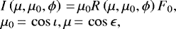
In what follows, we summarize the key parts of the present model for the surface reflection coefficient (Muinonen et al. 2020). The emergent intensity relates to the diffuse reflection coefficient, R, of an asteroid’s surface element as
 (1)
(1)
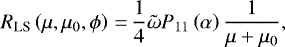
where πF0 is the incident flux density, ι and ϵ are the angles of incidence and emergence, and ϕ denotes the azimuthal angle between the directions of incidence and emergence. We use the Lommel-Seeliger reflection coefficient (Lumme & Bowell 1981; Wilkman et al. 2015),
 (2)
(2)
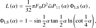
where  is the single-scattering albedo, P11 is the single-scattering phase function, and α is the phase angle. Then, the disk-integrated brightness, L, of a spherical asteroid can be written as
 (3)
(3)
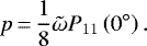
where D is the diameter of the asteroid and the phase function,  , is normalized to unity at zero phase angle. The geometric albedo, p, for a Lommel-Seeliger sphere is
 (4)
(4)
When using the model
 (5)
(5)
we get
 (6)
(6)
which is useful in analyzing asteroid phase curves since the normalization to the Lommel-Seeliger phase curve of a spherical asteroid does not depend on the shape to be derived.
As the phase dependence for 10° ≤ α ≤ 50° on the magnitude scale is approximately linear, we characterize the phase curve using a single slope parameter, βS, in the proximity of a phase angle α0:
 (7)
(7)
The βS parameter is closely related to the single-scattering phase function of an asteroid’s surface element. It describes the phase curve slope for a fictitious spherical asteroid that has a reflection coefficient that coincides with that of the real nonspherical asteroid. Thus, βS can be termed the proper phase curve slope.
In the case of general convex shape models, we use the vector  to present an asteroid’s rotation, size, shape, and scattering parameters at a given epoch, t0, where the parameters are the rotation period, ecliptic pole longitude, ecliptic pole latitude, rotational phase at t0, spherical harmonics coefficients
  for the Gaussian surface density, geometric albedo, two parameters of the H, G1, G2 phase function, and the diameter, D. In this work, the geometric albedo, p, and the diameter, D, are omitted from the parameters in the case of both convex and ellipsoid inversion. Furthermore, since the convex shape model accounts for any changes in ϕ0, it is an unnecessary parameter. For the triaxial ellipsoidal shape models, the given parameters are
  , where a, b, and c are the ellipsoid semiaxes.
As the photometric measurements that we utilize from GDR2 do not constitute an extensive set of measurements from small to large phase angles, a two-parameter H, G12 phase function that includes G12 in the parameter set must be used. It follows that the parameters for the convex shapes are  , and for the triaxial ellipsoid shapes they are
  . Additionally, since we are interested in the slope parameter, βS, we replace G12 with βS, as previously demonstrated by Cellino et al. (2009), Santana-Ros et al. (2015), and Muinonen et al. (2020). However, here we further take the phase-angle distribution of the observations into account (see Eq. (7)).
It is necessary to extend the original definition of the H, G12 phase function (Muinonen et al. 2010) to both small, negative and large, positive values of G12. In the former case, based on Eq. (23) in Muinonen et al. (2010), we rule out increasing brightness with increasing phase angle. In the latter case, we enforce the absence of an opposition effect for G12 values that would result in negative weights, 1 − G1 − G2. Consequently,
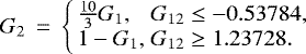 (8)
(8)
The extension does not affect the H, G12 phase function within its approximate nominal range of 0 ≤ G12 ≤ 1. Particular caution is called for in the application of G12 values far outside the nominal range.
The triaxial ellipsoidal shape model, the general convex shape model, and the inverse methods, such as the virtual-observation Markov chain Monte Carlo (MCMC) sampling, used in this study are described in detail by Muinonen et al. (2020).
2.2 Absolute magnitude and phase curve retrieval
We devised an algorithm for the derivation of absolute magnitudes and phase curves that allows for a consistent comparison between large numbers of asteroids. First, we started from the proper phase curve slope parameter, βS, retrieved from MCMC inversion, recognizing that βS describes the intrinsic surface element properties of each asteroid. Second, with the help of the full asteroid model available from the inversion, we moved to the reference geometry of equatorial illumination and observation (Kaasalainen et al. 2001) at the epochs and phase angles of the individual sparse GDR2 photometric points. Third, by studying the asteroid model brightnesses over one full rotation for each epoch, we determined the magnitudes of light curve brightness maxima. We then carried out linear least-squares fitting to determine the phase curve slope parameter, βmax. That parameter mimics the one commonly derived from ground-based observations, which was utilized in the derivation of the H, G1, G2 and H, G12 phase functions (see Table 1; we recall that βmax also depends on the phase-angle distribution). Fourth, matching βmax with the slope of the H, G12 phase function allowed us to unambiguously calculate the G12 parameter. This is justified by the piecewise linear phase curve dependence across the phase-angle range. Fifth, the H, G12 phase function then allowed us to predict the magnitudes based on brightness maxima for any selection of phase angles within 0°–120°. Sixth, in order to obtain a phase curve that corresponds to the intrinsic properties of the asteroids better, a reference phase curve was computed for the selected phase angles by averaging the magnitudes over one full rotation.
When the phase curve retrieval described above is carried out by utilizing true G-band magnitudes from GDR2, the projection of the reference phase curve to the zero phase angle immediately provides the absolute G-band magnitude. Finally, we computed the slope of the mean-magnitude reference phase curve at the 20° phase angle, βref. Repeating the computations for all the MCMC solutions allows us to obtain uncertainty estimates for the absolute magnitudes and phase curves.
Photometric phase curve slope parameter βmax(α = 20°), referring to light curve brightness maxima, for the G1, G2 values of different Tholen taxonomic classes (Penttilä et al. 2016).
3 Results and discussion
3.1 Observational data
As it is not possible to derive precise pole orientations from the photometry of GDR2 only (see Muinonen et al. 2020; Cellino et al. 2019), we performed the asteroid light curve inversion described in Sect. 2 for 491 asteroids using both the sparse photometric measurements from GDR2 and ground-based observations with initial rotation periods, longitudes, and latitudes from DAMIT. The intersection of GDR2 and DAMIT consists of 2479 asteroids. The asteroids were selected so that each of them has Gaia observations clustered around at least three different values of phase angle; the absolute rms values for the least-squares solutions of the Gaia data should be smaller than or equal to 0.015 mag and the absolute residual values smaller than or equal to 0.025 mag. Furthermore, we required at least six Gaia observations and at least two light curves for each target. We omitted the Lowell Observatory data (Oszkiewicz et al. 2011) because they have large uncertainties and the observationswere carried out without a filter. The slope changes are so subtle that we want to make sure that no further uncertainties are introduced by, for example, differences in bands or filters. Altogether, 491 asteroids were chosen for the light curve inversion. The results for all of the asteroids are available from the Strasbourg Astronomical Data Center (CDS). For demonstration purposes, we selected 12 asteroids that contain a variation of different Tholen (Tholen 1989) and Bus-DeMeo (DeMeo et al. 2009) taxonomic classes, different phase-angle ranges, and varying amounts of Gaia observations and ground-based light curves (see Table 2).
Example asteroids.
3.2 Application of the methods
3.2.1 Slope parameters
We performed convex and triaxial ellipsoid inversion for all 491 asteroids. For each asteroid, the initial parameters (see Sect. 2.1.) were set so that the rotation period, ecliptic pole longitude, and ecliptic pole latitude are the model parameters retrieved from DAMIT. Furthermore, we set the value of the initial slope parameter, βS, to 1.75 mag rad−1 as it is on the border of the slope values for various Tholen classes (see Table 1) and changing the value does not significantly affect the results.
For the triaxial ellipsoid shapes, we obtained least-squares solutions using the Nelder-Mead simplex algorithm to find the best-fit slope parameter values, rotational phase, and semiaxes b and c. We generated 10 000 virtual observations by adding Gaussian random errors to the true observations and applied the MCMC method to sample the slope parameter using 10 000 MCMC sample solutions for each asteroid. For the convex shapes, we took the least-squares solutions computed using the triaxial ellipsoid shapes as the starting point and then derived least-squares solutions using Levenberg-Marquardt optimization. We utilized 1000 virtual least-squares solutions and generated 5000 MCMC sample solutions for each asteroid to sample the spin, shape, and scattering parameters. The computing time used for one asteroid varied between one and five days on a single CPU core, depending on the amount of observations. The total computing time for 491 asteroids was more than 2000 days. In Fig. 1, we illustrate the photometric light curves with the best-fit convex model light curves for (376) Geometria. The goodness of the fit was generally better when there were more available Gaia data points and ground-based observations.
The computed maximum-based phase curve slopes, βmax, the mean-magnitude reference phase curve slopes, βref, and the proper phase curve slopes, βS, derived using both convex and ellipsoid shapes for our selected 12 example asteroids are presented in Table 3 together with their 1σ uncertainties. The dominating factors of the uncertainties are the amounts of Gaia observations and ground-based light curves,as well as the amount of apparitions. Generally, convex inversion produces more realistic βS values than ellipsoid inversion. Assuming an ellipsoid shape for all of the asteroids is not realistic. This can be seen in the results, which is why we focus on analyzing the slope parameters obtained by using convex inversion.
In Fig. 2 we present the histogram distributions of the computed βS, βmax, and βref values. The phase curve slope, βmax, based on light curve brightness maxima could be obtained for 345 asteroids. This is because we approximated the phase dependence on the magnitude scale to be linear; however, our data set contains massive amounts of targets with a wide range of phase angles. It is inevitable that there are targets that have nonlinear phase curves. The histograms show that the βS values are more spread than the βmax and βref values. Both βS and βmax refer to varying phase-angle ranges. The βS values range from 0.2 to 4.9, whereas the βmax and βref values do not contain any values below 1 and are concentrated in a realistic range of 1.2–2.5. Table 3 shows that the βS values derived using convex inversion are larger than the obtained βmax values for all of the selected example asteroids, in agreement with the increase in light curve amplitude with increasing phase angle (Zappalà et al. 1990).
We present the derived uncertainties for the slope parameter βref as a function of the respective slope parameter value in Fig. 3. In order to get a better picture of the results, we also show the known Tholen classes for 134 asteroids. The current Tholen and Bus-DeMeo asteroid taxonomies are presented in Table 4.
The results show that all of the asteroid complexes are widely spread and, to an extent, overlap with each other. However, S-complex and C-complex asteroids can be divided into two distinctive groups, whereas the X-complex asteroids and end members do not form any obvious groups. The reason why the X-complex and end members are so spread may be due to the fact that both groups are heterogeneous, comprising objects that have different compositions and albedos. According to Mahlke et al. (2021), the H, G1, G2 system can separate the different classes forming the X-complex based on phase curves, whereas this is not possible using the H, G12 system.
Taxonomic classification based on slope parameters alone is challenging as there are no clear boundary values between the taxonomic classes, and thus different types overlap. However, slopes can be used to complement the existing spectroscopic classifications, which is why comparing the retrieved slope values with the Bus-DeMeo taxonomic classification is important. Some of the asteroids may have been misclassified into an incorrect Tholen class. For example, asteroid (731) Sorga is a Tholen CD-type but a Bus-DeMeo Xe-type, indicating a high albedo that is distinct from C-types and D-types. The phase-angle range for (731) Sorga is 11.9°–18.7°, and the βmax value, 1.64 mag rad−1, is close to the asteroid’s computed βmax value at α = 20°. The derived value indicates that the asteroid is more likely an X-complex asteroid rather than an end member asteroid or a C-complex asteroid. Table 3 shows that the slope parameter values have large variations within the same Tholen class. Additionally, the uncertainties for the βS values are higher when using ellipsoid shapes.
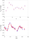 |
Fig. 1 Photometric light curves for asteroid (376) Geometria. The Gaia light curve is in the upper figure and a ground-based light curve #1 is in the bottom figure (blue circles). Red crosses stand for the best-fit convex model light curves with the 1σ uncertainties (red bars), and red points are the uncertainty envelopes using 5000 MCMC sample solutions. t and k describe the time and light curve observation count, and m0−m is the relative magnitude, where m0 = 0. |
Computed brightness-maximum-based phase curve slopes, βmax (mag rad−1), the mean-magnitude reference phase curve slopes, βref (mag rad−1), and the βS (mag rad−1) retrieved using convex inversion (CXI) and ellipsoid inversion (EI) with the 1σ uncertainties.
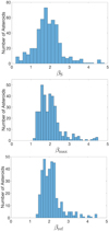 |
Fig. 2 Histograms of the derived βS, βmax, and βref values. 491 asteroids were used to obtain the βS values, whereas, the βmax and βref values were derived using 345 asteroids. |
3.2.2 Absolute magnitudes and phase curves
Absolute magnitudes and reference phase curves were computed for 345 asteroids. The derived G(1, 0) values for the 12 example asteroids are listed in Table 5 together with the 1σ uncertainties, the absolute magnitudes H retrieved from the JPL Small-Body Database, and the derived G1 and G2 parameters for the reference phase curves. Before carrying out comparisons, it should be noted that our G(1, 0) magnitudes were retrieved in the G-band, whereas the H magnitudes were obtained in the V-band. Gaia’s G-band (Evans et al. 2018) covers a wavelength region from ultraviolet (330 nm) to near infrared (1050 nm) with a full width half maximum of around 450 nm and a peak intensity at around 595 nm. The wavelength range in the V-band is approximately from 500 to 700 nm with a full width half maximum of 88 nm and a peak intensity at 550 nm.
All of the derived G(1, 0) magnitudes are fairly close to the H values (see Fig. 4). Small differences are expected because we are comparing magnitudes defined using two different photometric systems. The computed G(1, 0) for asteroid (402) Chloë shows the largest deviation, −0.65 mag, from its respective H value. The uncertainty of the derived G(1, 0) value is 0.0296 mag, and the G-V color difference for the Bus-DeMeo L-type asteroid is −0.224 mag, indicating that the H value retrieved from the JPL is likely wrong. As Chloë is a Barbarian asteroid (see Devogèle et al. 2018), it has unusual polarimetric properties and its phase curve could be more complicated than those of usual objects. In Fig. 5, we present the reference phase curves along with the H, G1, G2 fits for asteroids (55) Pandora, (95) Arethusa, (245) Vera, (596) Scheila, (731) Sorga, and (1251) Hedera, each of them from a different Tholen class. All of the magnitude points can be fitted well using phase angles 0.0°, 0.3°, 1.0°, 4.0°, 8.0°, 12.0°, 20.0°, 30.0°, and 50.0°. In general, the reference phase curves look similar, with small differences. Surprisingly, the M-type and S-type asteroids, (55) Pandora and (245) Vera, show steeper slopes than the E-type asteroid, (1251) Hedera. This is most likely caused by the choice of phase angles. If we omit the phase angle 50.0°, the slope would be steeper for all of the example asteroids.
The H, G1, G2 fits were obtained for 312 asteroids due to some of the asteroids showing extremely steep slopes. The H, G1, G2 system cannot fit these kinds of data well. Figure 6 shows the derived G1 and G2 parameters for different Tholen classes together with the line depicting the G12 dependence on the G1, G2 distribution that is based on the light curve brightness maxima (Muinonen et al. 2010). We have omitted the uncertainties of the G1 and G2 parameters because they are related to the chosen phase angles. The G1 and G2 parameters can be used to distinguish two groups: The first group contains M-type and S-type asteroids with moderate albedos, as well as D-type asteroids with low albedos. The second group contains P-, C-, X-, G-, and F-types that have low albedos. We have also included A- E-, T-, B-, and Q-types that each had only one target. The T-type asteroid and the E-type high-albedo asteroid can be grouped together with the first group, whereas, the B-type asteroid belongs to the second group. The A-type and the Q-type asteroids are separated from the other groups; however, as each of them represents a single asteroid, the uncertainties can be large. Figure 7 shows a few different Tholen classes in the G1 and G2 parameter space and their shifts from the G1 and G2 parameters that are based on light curve brightness maxima. The results indicate that all of the Tholen classes are shifted downward and to the right (see Zappalà et al. 1990).
Tholen and Bus-DeMeo asteroid taxonomic classification and the number of analyzed asteroids, Na, for each complex based on Tholen taxonomy.
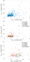 |
Fig. 3
|


Tholen classes, the derived G-band absolute magnitudes, G(1, 0), at the opposition and their uncertainties, σG, the absolute magnitudes, H, retrieved from the JPL Small-Body Database, the derived absolute magnitudes, HG, using the H, G1, G2 fit, and the derived G1 and G2 parameters for the reference phase curves.
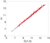 |
Fig. 4 Comparison of the derived G-band absolute magnitudes G(1, 0) and the V-band absolute magnitudes H based on the Jet Propulsion Laboratory Small-Body Database for 345 asteroids. The blue line represents perfect correlation of the absolute magnitudes. |
3.2.3 Rotation
Along with the slope parameters presented in Table 3, rotational periods and pole ecliptic longitudes and latitudes were retrieved. Table 6 shows the derived values with their 1σ uncertainties using convex shapes. For most of the targets, the parameters differ slightly from those in DAMIT; however, plenty of asteroids have several modeled values in DAMIT, and our computations give a good indication of what the best modeled values are. Finally, we can compare our results with that of one object: (95) Arethusa, which was analyzed by Cellino et al. (2019) using GDR2 data only and adopting both a triaxial ellipsoid and a “Cellinoid” shape model. The spin period of 8.7022 h obtained using convex inversion is in a good agreement with the triaxial ellipsoid spin period of 8.7015 h and the Cellinoid spin period of 8.7049 h.
4 Conclusions
We applied light curve inversion to 491 asteroids using photometric measurements from GDR2 and ground-based data from DAMIT. The retrieved slope parameters were presented and further analyzed while taking different Tholen taxonomic classes into account. As our data set contained few high-albedo asteroids, they are left to be studied in future work.We conclude that the global shapes of the asteroids and the roughness on all scales affect the derived βS.
We introduced the retrieval of absolute magnitudes and reference phase curves from Gaia data. The derived absolute magnitudes were compared with those obtained from the JPL Small-Body Database. We note that the absolute magnitudes and phase curves were derived in the G-band, which causes differences when compared to the V-band. In future studies, the derived values should be transformed to the V-band for a proper comparison.
It is clear that the present approach allows for an extensive computation of reference phase curves from the GDR2 and forthcoming GDR3 photometric data. With the help of ground-based observations, it will be possible to derive surface single-scattering phase functions for a large number of asteroids. Indeed, the detailed shapes of these phase functions are an interesting future topic of research.
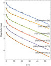 |
Fig. 5 The photometric reference phase curves with the H, G1, G2 fits for asteroids (55) Pandora, (95) Arethusa, (245) Vera, (596) Scheila, and (1251) Hedera. For illustration, the reference phase curves are presented on a relative magnitude scale with 0.5-mag offsets. |
Derived rotation periods, P (h), longitudes, λ(°), and latitudes, β(°), with their 1σ uncertainties,using convex inversion on a selection of asteroids.
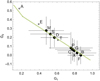 |
Fig. 6 The distributions of the different Tholen classes (black dots) and the uncertainties within the classes (black crosses) in the G1 and G2 parameter space based on the reference phase curves. The grey dots represent single asteroids and the green line shows how the G12 parameter maps into G1 and G2 in the H, G12 magnitude system. |
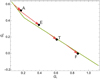 |
Fig. 7 The average G1 and G2 parameters of a few Tholen classes (black dots). The green line shows how the G12 parameter maps into G1 and G2 in the H, G12 magnitude system and the red arrows show the shifts from the light curve maximum based G1 and G2 parameters. |
Acknowledgements
This work was supported by the Academy of Finland grant No. 1325805 and the Chinese Academy of Sciences grant No. 2021VMA0017. We would like to thank the anonymous referee and Grigori Fedorets for constructive comments.
References
- Cellino, A., Hestroffer, D., Tanga, P., & Dell’Oro, A. 2009, in SF2A-2009: Proceedings of the Annual meeting of the French Society of Astronomy and Astrophysics, eds. M. Heydari-Malayeri, C. Reylé, & R. Samadi, 37 [Google Scholar]
- Cellino, A., Hestroffer, D., Lu, X. P., Muinonen, K., & Tanga, P. 2019, A&A, 631, A67 [CrossRef] [EDP Sciences] [Google Scholar]
- DeMeo, F. E., Binzel, R. P., Slivan, S. M., & Bus, S. J. 2009, Icarus, 202, 160 [NASA ADS] [CrossRef] [Google Scholar]
- Devogèle, M., Tanga, P., Cellino, A., et al. 2018, Icarus, 304, 31 [NASA ADS] [CrossRef] [Google Scholar]
- Durech, J., Sidorin, V., & Kaasalainen, M. 2010, A&A, 513, A46 [NASA ADS] [CrossRef] [EDP Sciences] [Google Scholar]
- Evans, D. W., Riello, M., De Angeli, F., et al. 2018, A&A, 616, A4 [NASA ADS] [CrossRef] [EDP Sciences] [Google Scholar]
- Gaia Collaboration (Brown, A. G. A., et al.) 2018a, A&A, 616, A1 [NASA ADS] [CrossRef] [EDP Sciences] [Google Scholar]
- Gaia Collaboration (Spoto, F., et al.) 2018b, A&A, 616, A13 [NASA ADS] [CrossRef] [EDP Sciences] [Google Scholar]
- Harris, A. W., Young, J. W., Contreiras, L., et al. 1989, Icarus, 81, 365 [NASA ADS] [CrossRef] [Google Scholar]
- Kaasalainen, M., Torppa, J., & Muinonen, K. 2001, Icarus, 153, 37 [Google Scholar]
- Kaasalainen, S., Piironen, J., Kaasalainen, M., et al. 2003, Icarus, 161, 34 [NASA ADS] [CrossRef] [Google Scholar]
- Lumme, K., & Bowell, E. 1981, AJ, 86, 1694 [NASA ADS] [CrossRef] [Google Scholar]
- Mahlke, M., Carry, B., & Denneau, L. 2021, Icarus, 354, 114094 [Google Scholar]
- Muinonen, K., Belskaya, I. N., Cellino, A., et al. 2010, Icarus, 209, 542 [NASA ADS] [CrossRef] [Google Scholar]
- Muinonen, K., Torppa, J., Wang, X. B., Cellino, A., & Penttilä, A. 2020, A&A, 642, A138 [EDP Sciences] [Google Scholar]
- Oszkiewicz, D., Muinonen, K., Bowell, E., et al. 2011, J. Quant. Spectr. Rad. Transf., 112, 1919 [NASA ADS] [CrossRef] [Google Scholar]
- Penttilä, A., Shevchenko, V. G., Wilkman, O., & Muinonen, K. 2016, Planet. Space Sci., 123, 117 [Google Scholar]
- Santana-Ros, T., Bartczak, P., Michałowski, T., Tanga, P., & Cellino, A. 2015, MNRAS, 450, 333 [NASA ADS] [CrossRef] [Google Scholar]
- Shevchenko, V. G., Belskaya, I. N., Muinonen, K., et al. 2016, Planet. Space Sci., 123, 101 [Google Scholar]
- Tholen, D. J. 1989, in Asteroids II, eds. R. P. Binzel, T. Gehrels, & M. S. Matthews (Tucson: University of Arizona Press), 1139 [Google Scholar]
- Wilkman, O., Muinonen, K., & Peltoniemi, J. 2015, Planet. Space Sci., 118, 250 [Google Scholar]
- Zappalà, V., Cellino, A., Barucci, A. M., Fulchignoni, M., & Lupishko, D. F. 1990, A&A, 231, 548 [Google Scholar]
All Tables
Photometric phase curve slope parameter βmax(α = 20°), referring to light curve brightness maxima, for the G1, G2 values of different Tholen taxonomic classes (Penttilä et al. 2016).
Computed brightness-maximum-based phase curve slopes, βmax (mag rad−1), the mean-magnitude reference phase curve slopes, βref (mag rad−1), and the βS (mag rad−1) retrieved using convex inversion (CXI) and ellipsoid inversion (EI) with the 1σ uncertainties.
Tholen and Bus-DeMeo asteroid taxonomic classification and the number of analyzed asteroids, Na, for each complex based on Tholen taxonomy.
Tholen classes, the derived G-band absolute magnitudes, G(1, 0), at the opposition and their uncertainties, σG, the absolute magnitudes, H, retrieved from the JPL Small-Body Database, the derived absolute magnitudes, HG, using the H, G1, G2 fit, and the derived G1 and G2 parameters for the reference phase curves.
Derived rotation periods, P (h), longitudes, λ(°), and latitudes, β(°), with their 1σ uncertainties,using convex inversion on a selection of asteroids.
All Figures
|
Fig. 1 Photometric light curves for asteroid (376) Geometria. The Gaia light curve is in the upper figure and a ground-based light curve #1 is in the bottom figure (blue circles). Red crosses stand for the best-fit convex model light curves with the 1σ uncertainties (red bars), and red points are the uncertainty envelopes using 5000 MCMC sample solutions. t and k describe the time and light curve observation count, and m0−m is the relative magnitude, where m0 = 0. |
| In the text | |
|
Fig. 2 Histograms of the derived βS, βmax, and βref values. 491 asteroids were used to obtain the βS values, whereas, the βmax and βref values were derived using 345 asteroids. |
| In the text | |
|
Fig. 3
|
| In the text | |
|
Fig. 4 Comparison of the derived G-band absolute magnitudes G(1, 0) and the V-band absolute magnitudes H based on the Jet Propulsion Laboratory Small-Body Database for 345 asteroids. The blue line represents perfect correlation of the absolute magnitudes. |
| In the text | |
|
Fig. 5 The photometric reference phase curves with the H, G1, G2 fits for asteroids (55) Pandora, (95) Arethusa, (245) Vera, (596) Scheila, and (1251) Hedera. For illustration, the reference phase curves are presented on a relative magnitude scale with 0.5-mag offsets. |
| In the text | |
|
Fig. 6 The distributions of the different Tholen classes (black dots) and the uncertainties within the classes (black crosses) in the G1 and G2 parameter space based on the reference phase curves. The grey dots represent single asteroids and the green line shows how the G12 parameter maps into G1 and G2 in the H, G12 magnitude system. |
| In the text | |
|
Fig. 7 The average G1 and G2 parameters of a few Tholen classes (black dots). The green line shows how the G12 parameter maps into G1 and G2 in the H, G12 magnitude system and the red arrows show the shifts from the light curve maximum based G1 and G2 parameters. |
| In the text | |
Current usage metrics show cumulative count of Article Views (full-text article views including HTML views, PDF and ePub downloads, according to the available data) and Abstracts Views on Vision4Press platform.
Data correspond to usage on the plateform after 2015. The current usage metrics is available 48-96 hours after online publication and is updated daily on week days.
Initial download of the metrics may take a while.