| Issue |
A&A
Volume 649, May 2021
|
|
|---|---|---|
| Article Number | A52 | |
| Number of page(s) | 19 | |
| Section | Cosmology (including clusters of galaxies) | |
| DOI | https://doi.org/10.1051/0004-6361/201937312 | |
| Published online | 12 May 2021 | |
Validating the Fisher approach for stage IV spectroscopic surveys
1
Université de Toulouse, UPS-OMP, IRAP and CNRS, IRAP, 14, avenue Edouard Belin, 31400 Toulouse, France
e-mail: This email address is being protected from spambots. You need JavaScript enabled to view it.
2
Dipartimento di Fisica, Università degli Studi di Torino, Via P. Giuria 1, 10125 Torino, Italy
3
INFN – Istututo Nazionale di Fisica Nucleare, Sezione di Torino, Via P. Giuria 1, 10125 Torino, Italy
4
INAF – Istituto Nazionale di Astrofisica, Osservatorio Astrofisico di Torino, Strada Osservatorio 20, 10025 Pino Torinese, Italy
5
AIM, CEA, CNRS, Université Paris-Saclay, Université Paris Diderot, Sorbonne Paris Cité, 91191 Gif-sur-Yvette, France
6
Université PSL, Observatoire de Paris, Sorbonne Université, CNRS, LERMA, 75014 Paris, France
7
CEICO, Institute of Physics of the Czech Academy of Sciences, Na Slovance 2, Praha 8, Czech Republic
8
Jet Propulsion Laboratory, California Institute of Technology, 4800 Oak Grove Dr, Pasadena, CA 91109, USA
9
School of Physics and Astronomy, Queen Mary University of London, Mile End Road, London E1 4NS, UK
10
Université St Joseph; UR EGFEM, Faculty of Sciences, Beirut, Lebanon
11
Departamento de Física, FCFM, Universidad de Chile, Blanco Encalada 2008, Santiago, Chile
12
Institute of Space Sciences (ICE, CSIC), Campus UAB, Carrer de Can Magrans, s/n, 08193 Barcelona, Spain
13
Institut d’Estudis Espacials de Catalunya (IEEC), 08034 Barcelona, Spain
Received:
13
December
2019
Accepted:
28
July
2020
Abstract
In recent years, forecasting activities have become an important tool in designing and optimising large-scale structure surveys. To predict the performance of such surveys, the Fisher matrix formalism is frequently used as a fast and easy way to compute constraints on cosmological parameters. Among them lies the study of the properties of dark energy which is one of the main goals in modern cosmology. As so, a metric for the power of a survey to constrain dark energy is provided by the figure of merit (FoM). This is defined as the inverse of the surface contour given by the joint variance of the dark energy equation of state parameters {w0, wa} in the Chevallier-Polarski-Linder parameterization, which can be evaluated from the covariance matrix of the parameters. This covariance matrix is obtained as the inverse of the Fisher matrix. The inversion of an ill-conditioned matrix can result in large errors on the covariance coefficients if the elements of the Fisher matrix are estimated with insufficient precision. The conditioning number is a metric providing a mathematical lower limit to the required precision for a reliable inversion, but it is often too stringent in practice for Fisher matrices with sizes greater than 2 × 2. In this paper, we propose a general numerical method to guarantee a certain precision on the inferred constraints, such as the FoM. It consists of randomly vibrating (perturbing) the Fisher matrix elements with Gaussian perturbations of a given amplitude and then evaluating the maximum amplitude that keeps the FoM within the chosen precision. The steps used in the numerical derivatives and integrals involved in the calculation of the Fisher matrix elements can then be chosen accordingly in order to keep the precision of the Fisher matrix elements below this maximum amplitude. We illustrate our approach by forecasting stage IV spectroscopic surveys cosmological constraints from the galaxy power spectrum. We infer the range of steps for which the Fisher matrix approach is numerically reliable. We explicitly check that using steps that are larger by a factor of two produce an inaccurate estimation of the constraints. We further validate our approach by comparing the Fisher matrix contours to those obtained with a Monte Carlo Markov chain (MCMC) approach – in the case where the MCMC posterior distribution is close to a Gaussian – and finding excellent agreement between the two approaches.
Key words: dark energy / cosmological parameters / large-scale structure of Universe / galaxies: statistics
© S. Yahia-Cherif et al. 2021
 Open Access article, published by EDP Sciences, under the terms of the Creative Commons Attribution License (https://creativecommons.org/licenses/by/4.0), which permits unrestricted use, distribution, and reproduction in any medium, provided the original work is properly cited.
1. Introduction
Since the discovery of the acceleration of the expansion of the Universe in the late 1990s (Riess et al. 1998; Perlmutter et al. 1999), the Lambda Cold Dark Mattery (ΛCDM) model remains the most successful model in cosmology. It provides a simple and accurate description of the properties of the Universe, with a very limited number of parameters that are now constrained at the level of a few percent by using measurements from the Planck CMB mission (Planck Collaboration VI 2020) and other experiments (see e.g., Percival et al. 2001; Blake et al. 2011; Alam et al. 2017; Abbott et al. 2018). The accelerated expansion of the Universe can be explained by postulating a new form of matter or the mechanism dubbed “dark energy”, which would be present alongside dark matter. Dark energy dominates the energy budget of the Universe today, making up for ∼70% of its total energy density.
Over the past two decades, a range of dark energy experiments have been proposed in order to study the observed cosmic acceleration of the Universe through various probes: optical spectroscopic and photometric galaxy clustering, and weak gravitational lensing, supernovae, with galaxy clusters being the most common. In order to quantify the performance of a survey and, in particular, its ability to constrain the properties of dark energy, the Dark Energy Task Force (DETF) defined a metric known as the figure of merit (FoM, Albrecht et al. 2006): a figure inversely proportional to the surface bounded by the confidence contours for the w0 and wa parameters from the Chevalier-Polarski-Linder (CPL) parameterization (Chevallier & Polarski 2001; Linder 2003). The application of the FoM is now standard for quantifying the performance of a particular experiment that aims to constrain the dark energy parameters.
We are currently entering the era of high-precision cosmology with a suite of stage IV experiments that are about to be deployed. Currently, ongoing and forthcoming ground-based experiments as well as space missions include: DESI1 (DESI Collaboration 2016), Euclid2 (Laureijs et al. 2011; Amendola et al. 2018; Euclid Collaboration 2020), LSST3 (LSST Science Collaboration 2009; Ivezić et al. 2019; Chisari et al. 2019), WFIRST4 (Akeson et al. 2019; Dore et al. 2019), and the SKA5 (Square Kilometre Array Cosmology Science Working Group 2020). Forecasting activities are key for predicting future constraints on cosmological parameters and the corresponding dark energy FoM. Indeed, forecasts not only allow us to predict the performance of a future survey but also aid in its design and optimization.
There are a number of different ways to compute forecasts. For instance, it’s possible to use a simulated realization of the data and a Monte Carlo Markov chain (MCMC) method to sample the likelihood of the parameters of interest. This approach is known to provide reliable estimations of the constraints on the cosmological parameters (see e.g., Dunkley et al. 2005). However, it is often quite time-consuming, especially if there is a wide variety of cases involved. The Fisher matrix formalism, as adopted by the DETF, is a computationally fast approach that allows for constraints to be obtained within a few seconds or minutes. However, this method is dubious from the technical point of view as the covariance matrix is obtained by inversion of the Fisher matrix, whose coefficient calculations often require the computation of derivatives and integrals, which can lead to inaccurate results in cases where, for example, the step sizes (as we show in subsequent sections of this paper) are not chosen properly to ensure the appropriate precision. Moreover, the Fisher formalism can miss contour shapes and, thus, miss potential degeneracies (see e.g., Wolz et al. 2012) as it assumes a Gaussian likelihood in a frequentist approach or a Gaussian posterior of the parameters in a Bayesian approach; that might not be true if, for example, the parameters are not tightly constrained by the experiment(s). Several methods have been proposed to handle these complex situations (Joachimi & Taylor 2011; Sellentin et al. 2014; Sellentin 2015; Amendola & Sellentin 2016).
In the present study, we propose a numerical approach that is independent of the specific problem treated, with the purpose of testing the numerical reliability of constraints obtained within the Fisher matrix formalism. As a working example, we consider the spectroscopic galaxy clustering probe for the following stage IV surveys: DESI, Euclid, and WFIRST-2.4. The paper is organized as follows. In Sect. 2, we give a brief description of the aforementioned surveys. In Sect. 3, we describe the different tests performed in order to validate the Fisher approach: namely, we determine the required precision to compute a valid Fisher matrix, carry out several stability and convergence tests, and perform a comprehensive comparison with the MCMC approach. In Sect. 4, we present the results and address possible ways of numerically validating the Fisher matrix approach. Finally, we report our conclusions in Sect. 5.
2. Surveys
2.1. Euclid
Euclid is a medium-class ESA mission that is aimed at gaining an improved understanding of the expansion of the Universe, as well as dark energy and dark matter. Euclid will measure the shape of more than one billion galaxies and provide tens of millions of spectroscopic redshift. It will use two main cosmological probes, namely galaxy clustering and weak gravitational lensing. These will allow us to probe the dark sector of the Universe with unprecedented precision. Euclid (Laureijs et al. 2011) targets a FoM of 400, while also aiming to distinguish between different theories of gravity, that is, testing general relativity against alternative models by measuring the exponent of the growth factor, γ, with a precision higher than 0.02 at 1σ. Euclid will also measure the neutrino masses with a 1σ precision better than 0.03 eV. Combined with Planck, Euclid will also probe some inflation models through the measurement of the non-Gaussianity of initial conditions. So far, two surveys are planned: a wide one of 15 000 deg2 and a deep one of 40 deg2. The 1.2m telescope contains two instruments that will allow to observe around 2 billion galaxies and produce 50 million precise redshift measurements. Euclid’s large format visible imager (VIS), will probe the photometric galaxy clustering in the optical wavelength range. The near-infrared imaging and spectroscopy (NISP) instrument will perform photometry imaging and produce spectra in the near infrared range.
2.2. Dark Energy Spectroscopic Instrument (DESI)
Known as the successor of the stage III BOSS and eBOSS surveys (Dawson et al. 2013, 2016), DESI is a Stage IV ground-based dark energy experiment whose primary objectives are measuring the baryonic acoustic oscillations (BAO) and constraining the growth of structure through redshift space distortions measurements. It will allow for the estimation of the deviations from Gaussianity through the fNL parameter. DESI will also measure the neutrinos masses with a precision of 0.02 eV at 1σ, for a maximum scale of kmax < 0.2 h Mpc−1. It will scan a 14 000 deg2 sky area and measure more than 30 million spectra from four galaxy populations: the bright galaxies (BGS) at low redshift (until z ≤ 0.6), the luminous red galaxies (LRGs) composed of highly biased objects at intermediate redshift z < 1, the bright emission lines galaxies (ELGs) up to z = 1.7 (which can only be detected at high resolution since the OII doublet must be well-resolved), and the quasi-stellar objects (QSOs). The latter group allows us to trace both the matter distribution at high redshift and the neutral hydrogen by the Ly − α absorption in the spectra. DESI is now underway and will conduct observations over five years (2019–2023) using the Mayall four-meter telescope at Kitt Peak.
2.3. Wide Field Infrared Survey Telescope (WFIRST)
WFIRST is a NASA near-infrared imaging and low-resolution spectroscopy observatory that, similarly to Euclid, aims to address fundamental questions about the accelerated expansion of the Universe. WFIRST will determine the expansion history of the Universe and structure growth in order to constrain dark energy and modified gravity models. To estimate the dark energy equation of state, WFIRST will perform weak lensing, along with measurements of supernovae distance and baryonic acoustic oscillations. In this work, we use the spectroscopic probe of WFIRST-2.4, a 2000 deg2 survey that will observe more than 20 million galaxies in the redshift range of 1 ≤ z ≤ 3.
3. Methodology
3.1. The surveys combination specification
In general, using a single probe of a stage IV survey does not constrain cosmological parameters well enough to get a Gaussian posterior distribution, in which case testing simply the Fisher formalism is meaningless. However, when the constraints are very tight, the posterior is likely to be close to gaussian. For this reason, we chose to investigate the Fisher formalism in a case where we can anticipate a Gaussian posterior (an assumption that is checked by the MCMC forecast used for the full validation of the method). In order to substantially improve the constraints, we therefore combine Euclid, DESI, and WFIRST-2.4. However, we note that DESI and WFIRST-2.4 cover Euclid’s entire redshift range. Hence, if we want to fully and consistently combine these three surveys, computing the cross-correlation power spectra between those surveys is necessary. For the purposes of our study, we do not wish to consider the cross-spectra, therefore, we have to remove all the DESI and WFIRST-2.4 redshift bins that overlap with Euclid. In practice, we perform the full spectroscopic Euclid forecasts in the redshift range of 0.9 ≤ z ≤ 1.8, the DESI forecasts at low redshift 0 < z < 0.9, and the WFIRST-2.4 forecasts at high redshift 1.8 < z < 2.7. Moreover, between z = 0.6 and z = 0.9 the ELGs, LRGs, and QSOs populations from DESI also overlap. Each of these populations has a different bias and their cross-power spectra would have to be computed as well. For simplicity, we only consider the ELGs population at z = {0.6, 0.9} because it has the highest density of galaxies and potentially offers the best constraints on the parameters. At z < 0.6, we consider the BGS population.
We consider four redshift bins for the DESI survey with the following binning: 2 redshift bins for the BGS population centered at z = {0.125, 0.375} with a redshift size Δz = 0.25 and 2 redshift bins for the ELGs population centered at z = {0.6, 0.8} with Δz = 0.2. Both Euclid and WFIRST-2.4 utilise 3 redshift bins with Δz = 0.3, centered at z = {1.05, 1.35, 1.65} and z = {1.95, 2.25, 2.55}, respectively. The full binning procedure is summarized in Table 1.
Redshift range, binning choices, and density of galaxies for the surveys used in this work.
3.2. Two approaches towards Fisher matrix cosmological constraints
In this work, we follow two approaches for the Fisher matrix forecast of cosmological constraints using the galaxy clustering probe. We describe these two approaches, dubbed M1 and M2, below.
3.2.1. M1 approach
In the first approach, M1, the cosmological model considered, is an extension of the ΛCDM model in which we assume a variable dark energy equation of state parameter described by the CPL parameterization. Furthermore, we allow for non-flatness by letting ΩDE vary. We also assume massless neutrinos. The full set of cosmological parameters is:
θcosmo : {Ωb, h, Ωm, ns, ΩDE, w0, wa, σ8}.
The cosmological parameters are the quantities of direct interest here. Ωb, h, Ωm, ns are parameters that modulate the shape of the power spectrum. Ωb is the baryon density parameter. The h is the reduced Hubble constant defined as h = H0/(100 km s−1 Mpc−1), where H0 is the present day Hubble parameter. Ωm is the matter density parameter, and ns the spectral scalar index. The ΩDE is the dark energy content directly linked to the curvature of the universe and (w0, wa) represent, respectively, the dark energy equation of state at z = 0 and its derivative with respect to scale factor at z = 0, in the so-called CPL form (Chevallier & Polarski 2001; Linder 2003). The equation of state is then given by:
 (1)
(1)
The σ8 parameter gives the amplitude of matter fluctuations in the linear regime on a scale of 8 h−1 Mpc. Furthermore, at each redshift bin, we consider two nuisance parameters: the logarithm of the product between the bias and σ8(z), namely, ln(bσ8), and the shot noise, Pshot(z), due to the finite self-pair counts in two-point statistics. The shot noise affects the power spectrum by adding a white systematic component increasing thus the statistical uncertainties. We consider 10 redshift bins, zi, thus, the total number of nuisance parameters amounts to 20:
θnuisance = {ln(bσ8(zi)), Pshot(zi)}.
The cosmological parameters fiducial values are summarized in Table 2 and the nuisance parameters are given in Table 3.
Fiducial values for the cosmological parameters (M1 approach).
Fiducial values for the nuisance parameters.
3.2.2. Approach M2
In the second approach, M2, adopted in the Euclid Collaboration (2020), four quantities which determine the shape of the power spectrum are treated as independent of the cosmological parameters. We call these four quantities the shape parameters. The other quantities, the angular diameter distance, Da(z), the Hubble rate, H(z), and the growth rate of cosmic structure, f(z) are called the redshift dependent (RD) parameters. With the addition of three redshift-dependent parameters and 2 redshift-dependent nuisance parameters (the same as in M1) per redshift bin, for ten redshift bins, this amounts to 30 redshift dependent parameters and 20 nuisance parameters. The full set consists of 54 parameters (see Table 4):
θshape : {ωb, h, ωm, ns}
θrd + nuisance : {ln(Da(zi)), ln(H(zi)), ln(fσ8(zi)), ln(bσ8(zi)), Pshot(zi)}.
The nuisance parameters are identical in the two approaches. As in the Euclid Collaboration (2020), we estimate the constraints of the physical baryon density (ωb = Ωbh2), and the physical matter density (ωm = Ωmh2) parameters. In the M2 approach, the constraints on the final cosmological parameters (θcosmo) are obtained from the 54 parameters stated above by projection. We also note that taking the logarithm of the parameters helps to stabilize matrix inversion by reducing the dynamic range between minimum and maximum eigenvalues, as described in Euclid Collaboration (2020).
Fiducial values of the shape and redshift dependent parameters for the approach M2.
3.3. The Fisher matrix formalism
The Fisher matrix formalism (see Coe 2009 for a pedagogical introduction) is commonly used in cosmology to forecast the Gaussian uncertainties of a set of model parameters under some constraints. The Fisher approach relies on the assumption of Gaussian posterior distribution. The Fisher matrix corresponding to the information on cosmological parameters provided by a galaxy clustering survey is given by (Tegmark 1997; Tegmark et al. 1998):
 (2)
(2)
where α and β run over the parameters we vary. k is the total wave vector magnitude in Mpc−1, μ the cosine of the angle to the line of sight, and Veff(z, k, μ) the effective volume of the survey:
![Mathematical equation: $$ \begin{aligned} V_{\rm eff}(z,k,\mu ) = V_{\rm s}(z)\left[\frac{n(z)P_{\rm obs}(z,k,\mu )}{n(z)P_{\rm obs}(z,k,\mu )+1}\right]^2 , \end{aligned} $$](/articles/aa/full_html/2021/05/aa37312-19/aa37312-19-eq4.gif) (3)
(3)
with n(z) the number density of galaxies in each redshift bin and Vs(z) the volume of each redshift bin. The observed power spectrum Pobs(z, k, μ), taking into account nonlinear effects is given by:
![Mathematical equation: $$ \begin{aligned}&P_{\rm obs}(z,k,\mu ) = \frac{1}{q_{\perp }^2q_{\parallel }} \left(\frac{[b\sigma _8(z)+f\sigma _8(z)\mu ^2]^2}{1 + [f(z)k\mu \sigma _{\rm p}(z)]^2}\right) \nonumber \\&\qquad \qquad \qquad \times \frac{P_{\mathrm{d}{ w}}(z,k,\mu )}{\sigma _8^2(z)}F_z(z,k,\mu ) + P_{\rm shot}(z) . \end{aligned} $$](/articles/aa/full_html/2021/05/aa37312-19/aa37312-19-eq5.gif) (4)
(4)
The first term represents the Alcock-Paczynski (AP) volume dilation effect that reflects spurious anisotropies in the power spectrum which arises when assuming a cosmology (that might be different from the true cosmology) to convert redshifts into distances. The coefficient q∥ = Href(z)/H(z) is given by the ratio between the Hubble parameter in the true cosmology and the one in the reference cosmology. The coefficient q⊥ = Da(z)/Da, ref(z) is given by the ratio between the angular distance in the reference cosmology and the one in the true cosmology. The term, between parentheses, contains the linear redshift space distortions due to the growth of structure and finger-of-God effects that aim to describe the nonlinear damping due to the velocity dispersion of satellite galaxies inside host halos. Then, σp = 1/(6π2)∫Pm(k, z)dk represents the linear theory velocity dispersion that can be computed from the linear matter spectrum Pm(k, z). The third term, Pdw, is the dewiggled power spectrum (Eisenstein & Hu 1998, 1999) that takes into account the nonlinearities in the matter power spectrum. The fourth term, Fz, represents the uncertainties coming from the spectroscopic precision of the survey under consideration and Pshot(z) the residual shot noise. For a comprehensive description of the observed power spectrum model introduced above, we recommend the recent Euclid paper on validated forecasts (Euclid Collaboration 2020), where the specific form of the function Fz as well as the rescaling of k and μ due to the AP effect are given in Eqs. (74)–(79). In terms of nonlinearities, we should note that the model used accounts for the finger-of-God effect as well as for the damping of the BAO feature. More details can be found in Sect. 3.2.2 of Euclid Collaboration (2020).
We move on to describing the estimation of the uncertainties using the Fisher matrix formalism. The inverse of the Fisher matrix gives the covariance matrix that represents the likelihood curvature evaluated at the fiducial values of α and β. According to the Cramér-Rao inequality, the square root of each covariance matrix diagonal elements gives the 1σ lower bound constraint for each parameter (marginalized over all other parameters) where the posterior distribution is Gaussian:
 (5)
(5)
In order to compute the Fisher matrix we use SpecSAF (Spectroscopic Super Accurate Forecast), a modified and improved version of a code first used in Tutusaus et al. (2016). SpecSAF computes high point stencil derivatives with a very high level of precision. This code is linked to CAMB (Lewis et al. 2000) and CLASS (Lesgourgues 2011) to compute the matter power spectra and allows the user to directly compute the FoM and plot the contours. We note that SpecSAF is one of the validated codes used in Euclid Collaboration (2020).
3.4. Precision of the Fisher matrix formalism
In order to obtain reliable final constraints from the covariance matrix, we have to estimate the precision needed for the Fisher elements themselves to achieve a given precision (for instance, a relative precision lower than 10% for the square root of elements of the diagonal of the covariance matrix). This problem is related to the conditioning of the Fisher matrix that needs to be inverted. The condition number ,CN, of a matrix, A, is known to provide an upper limit to the precision, δx, of the determination of the solution, x, of the equation, Ax = b, where b is a vector. That is, the elements of b and A have to be known with enough precision such that δbi/bi ≤ (1/CN) δx/x. That is, if the condition number is large, even a very small error in b will result in a large error in x. The condition number (Belsley et al. 2005) is given by the ratio between the largest eigenvalue to the smallest eigenvalue. This is however an upper limit that can be far too stringent in practice: as an example, in our case, the condition number in approach M1 is 1.3 × 10⁵, while in the M2 approach, the condition number is 4.4 × 10¹¹. This formally calls for a precision of ∼10−6 and ∼10−13 to ensure an accuracy of 10% in the final constraints. However, a diagonal matrix (provided that no term in the diagonal vanishes) is well-conditioned in practice, even if the condition number is very large. Therefore, for a matrix with size significantly greater that 2 × 2, the condition number does not provide useful information on the conditioning of the matrix. This observation has important consequences in practice, as the elements of the Fisher matrix are generally computed from numerical derivatives whose required precision has to be determined in order to achieve reliable results on the covariance. To better quantify the precision needed for reliable constraints we introduce a simple method that consists of “vibrating” each element of the Fisher matrix as follows:
 (6)
(6)
with α and β as the indices which run over all unique pairs of parameters. N(0, 1) is a normal distribution centered at 0 with variance 1 and ϵ the amplitude of the perturbations. In order to keep the Fisher matrix symmetric, we only perturb the lower triangle part of the Fisher and compute the symmetric part across the diagonal. The coefficients in the Fisher matrix are computed from Boltzmann codes and are therefore subjects to correlated noise. In our approach, this correlation is lost during the Fisher matrix vibration. In the approach M1, we apply the perturbations for 2000 amplitudes, ϵ, regularly logspaced in the range 10−12–10−1. To ensure enough statistical data and reduce the Poisson noise, we produce 10 000 vibrated Fisher matrix per epsilon values. In the M2 approach, this procedure is more expensive in terms of computational time. We therefore reduced the number of ϵ values to 600 in the range 10−6–10−1 and we produced 2000 vibrated Fisher matrices per ϵ value. The constraints obtained with each vibrated Fisher matrix are then compared with the original Fisher matrix by computing the relative error. For each parameter, we compute the number of draws that gives an agreement level on the constraints at the chosen precision (10% in our case) or better.
The tolerated precision is the largest value of ϵ for which 68% of the constraints on each parameter remain lower than the chosen precision (10% in our case). The results are illustrated in Fig. 1 for the cosmological parameters in the M1 approach. In the M2 approach, the size of the matrix is too large, so in Fig. 2 we only show the shape parameters and the redshift-dependent parameters for a single redshift bin (z = 1.35).
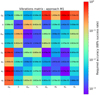 |
Fig. 1. Vibration matrix: approach M1. The values are expressed in absolute values. Each cell containing 1 has to be taken as a lower bound value of the limit because we take 1 as the threshold perturbation amplitude. |
3.5. Stability and convergence tests
The stability and convergence of numerical derivatives can be an important issue and testing it is an essential validation step. Fortunately, testing the stability of the derivative of the observed power spectrum over any parameter is straightforward and determines the appropriate step sizes to use and which ones to avoid. However, the stability itself does not prove that a numerical derivative is correctly computed since it only shows to what extent the derivative changes as a function of step size. Ideally, a convergence test, which consists in computing the relative error between the analytical derivative and the numerical one, also has to be performed. Unfortunately, directly exploiting the convergence with a relative error test is not possible when the derivatives cannot be computed analytically. This is the case for most of the parameters we consider in this study. For the cosmological parameters, we need to use a Boltzmann code and the semi-analytical form of the derivatives over Da(z) and H(z) contain derivatives of the matter power spectrum over the scale k (dP/dk). Here, we follow an alternative approach to test derivative convergence by considering three different numerical methods to compute the derivatives: the 3, 5, and 7 point-centered schemes. With the 3 (respectively 5, 7) scheme being the method in which we use 3 (respectively 5, 7) perturbed points of the function f(x) to determine the numerical derivative at x, we assume that the 7 points derivative is very near the true value when an appropriate step size is chosen. We compare the 7-point with the 3- and 5-point stencil for different step sizes and look for the best agreement between the two derivatives; in other words, we carry out convergence tests between the 3- and the 5-point stencil towards the 7 points stencil by comparing the relative error between the 7-point stencil and the 3- and 5-point stencils. More generally, the convergence is always faster with the high-stencil derivatives method than with the low-stencil derivatives, which means that the optimum for the 5-point stencil often occurs at larger step values than the 3-point stencil. However, this does not hold in all cases. For instance, applying this method to a highly noisy or oscillatory function can lead to erroneous results and finding stable behaviors would not be possible. It is therefore very useful to plot the functions under consideration in order to identify any such features.
3.6. The MCMC sampling
In order to consolidate the reliability of our Fisher matrix constraints, we compare them with MCMC constraints. As is well known, the MCMC sampling is much more time-consuming than the Fisher matrix computation due to the computational time needed to obtain the power spectrum at each iteration. Moreover, by construction, a Markov chain cannot be parallelized, as each draw depends on the previous displacement; however, it is possible to launch several chains at the same time to sample the parameter space more effectively. Considering a set of data and a model equipped with a set of parameters Θ, the MCMC allows us to use Bayesian inference and model comparison:
 (7)
(7)
with P(Θ|data) the posterior distribution, which provides the constraints and the joint covariance between all the parameters considered, P(data|Θ) the Likelihood, P(Θ) the prior that we take to be flat in the present study, and P(data) the Bayesian evidence that can be safely ignored as it is a constant of no interest in our situation. Thus, the previous equation can be reduced to:
 (8)
(8)
We compute the posterior distribution with the MCMC module of SpecSAF using the Metropolis-Hastings algorithm (Metropolis & Ulam 1949; Robert 2015). This is described in more detail in Appendix A. We test the chains convergence using the Gelman-Rubin diagnostic (Gelman & Rubin 1992; Brooks & Gelman 1998) described in Appendix B. Our data are modeled by the a realization of our fiducial model given by Eq. (4).
3.7. MCMC Comparison
The full validation of the Fisher matrix approach is performed with a direct comparison with the results from the MCMC chains. We sample the two parameter spaces of the two approaches and compare the relative error given by the covariance matrix of the sampling and the inverse of the Fisher matrix. We also visualize the Fisher contours versus the MCMC sampling. As we use exactly the same specifications for both methods, we expect to get the same constraints with a relative error lower than 10% as long as the posterior distribution remains gaussian and doesn’t present any degeneracies.
4. Results
4.1. Precision requirements
The vibration matrices for M1 and M2 are presented in Figs. 1 and 2, respectively. We can clearly see that the sensitivity of the constraints depends on the element vibrated. According to Fig. 1, the diagonal elements are the most sensitive, more specifically, Ωm, ΩDE and wa. For our working requested precision (10%), these three parameters require a precision between 0.06% and 0.09%; for the other parameters, the diagonal elements required precision spreads between 0.1% and 0.4%; the nondiagonal elements are less cumbersome: some of them can even change by a factor of 2 without affecting the constraints (for instance Ωb vs [ΩDE, w0, wa, σ8]). Most of the nondiagonal elements can be computed with a precision worse than 1%.
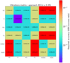 |
Fig. 2. Vibration matrix: approach M2. We note that some values are identical because we decreased the resolution of the perturbation amplitude range. |
The Fisher matrix produced following the M2 approach (Fig. 2) shows a greater sensitivity to vibration than the M1 approach, which is in line with their different condition numbers. The diagonal element, h, seems to be the most sensitive parameter with a required precision around 0.0012%, which is, however, much less stringent than what the condition number would suggest (∼10−11%). The background quantities and ωm require a precision around 0.015%, while ωb and ns are one order of magnitude more tolerant, with a target precision of 0.2%. The off-diagonal elements show a higher tolerance for perturbations, however, it is only the background elements versus [Ωb, ns] that demonstrate a vibration tolerance higher than one percent.
To summarize, compared to the M1 approach, the Fisher matrix produced in the M2 approach is generally at least two orders of magnitude more sensitive for the most sensitive parameters and one order of magnitude more sensitive for the less sensitive ones. These final figures are poorly reflected by the condition number of each approach. The above vibration matrix approach allows us to quantify the precision requested for the elements in the Fisher matrix to achieve the requested precision on the constraints of interest, namely, the FoM in our case. This effective precision is hard to anticipate otherwise: the condition number provides a mathematical lower limit to it. However, for a simple 2 × 2 diagonal matrix, it is clear that the precision needed for each element is just the one sought after with regard to the constraints, while the condition number (being the product of the eigenvalues) can be arbitrary large. The precision requested for the elements in the Fisher matrix is therefore intimately related to the internal structure of the Fisher matrix.
In the next section, we examine the step sizes necessary to achieve the requested accuracy on the Fisher matrix elements.
4.2. Stability and convergence
In order to compute the elements of the Fisher matrix (Eq. (2)), we have to compute several integral quantities involving the derivatives. The precision on these elements is therefore directly related to the precision that can be achieved on these computations, determined by the step sizes used and the numerical schemes used in these derivations. In the following, all the parameters step sizes shown are relative to their corresponding fiducial value, except for wa and Pshot and that is because their fiducial values is zero. Moreover, we chose to illustrate one shape parameter and one redshift dependent parameter in the following plots because the derivatives behavior between the shapes parameters is similar as well as the derivative behavior between the redshift-dependent parameters. We have therefore examined the precision obtained on each of these elements by first examining the precision reached when the step size varies. In order to illustrate this, we provide illustration for derivatives against step size, which are representative of general behavior. The upper panels of Fig. 3 illustrate the stability of the square of the derivative of lnP(k, μ) with respect to wa at (k, μ) = (0.0121, 0.5) and lnDa at (k, μ) = (0.098, −0.1) (blue: 3-point stencil, red: 5-point stencil, green: 7-point stencil), at z = 1.35. The upper left panel demonstrates the cosmological parameters stability behavior. The stability of the derivative is reached when the slope of the derivative value over the step size is close to zero (when the curve shows a horizontal behavior) while decreasing the step size. These derivatives are usually relatively stable in the step size range [10−4, 10−1] for each derivative. The truncation errors remain small in all of the range for most of the derivatives. We note that for the low step values, instabilities occur due to rounding errors. The upper-right panel is representative of the typical stability behavior of ln(H(z)) and ln(Da(z)). For step sizes higher than 3 × 10⁻³, instabilities begin to arise for the 3-point stencil. The truncation errors dominate and increase the total error budget. The instability range for the 5- and 7-point derivatives is smaller: typically around 1 × 10⁻². The lower panels (Fig. 3) represent the corresponding derivative convergence tests with respect to the 7-point derivatives; namely, the relative error between the 7-point stencil and the (3, 5) point stencil in (blue, red). Generally, convergence tests are carried out to compare the relative error between the analytical solution of a derivative and solutions obtained numerically when we vary the step size. The minimum relative error between the analytical form and the numerical solutions corresponds to the optimal step 6 that ensures the most accurate derivative. Because we cannot compute the analytical form of most of the derivatives presented here, we carry out convergence tests of the 5- and the 3-point stencil using the 7-point stencil results as a reference since the latter is theoretically more accurate. In the bottom-left panel, the 3-point derivative achieves its convergence when the step is equal to 10−2. The optimal step for the 5-point stencil is around 1 × 10⁻¹ at most. Concerning the angular diameter distance (bottom right panel), the 3-point convergence level is achieved down to a step of 3 × 10⁻⁷, whereas for the 5-point derivatives, it is around 5 × 10⁻⁵. Figure 3 shows that the convergence is always reached after the stability if we decrease the step size. For instance, let’s take a closer look on Fig. 3 right panel (lnDa(1.35)). If we observe the stability and the corresponding convergence plots at a step of 10−1, we see that the convergence and the stability aren’t reached yet. Now if we start to decrease the step size, we see that the stability is reached around a step of 10−2 because the slope of the curve becomes near to 0. However, the corresponding convergence plot still
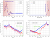 |
Fig. 3. Stability and convergence tests towards the 7-point stencil for wa and ln(Da(1.35)) at a given k and μ at z = 1.35. Upper left panel: stability of wa; upper right panel: stability of ln(Da(1.35)); bottom left panel: convergence of ωm; bottom right panel: convergence of ln(Da(1.35)). Blue: 3-point stencil, red: 5-point stencil, green: 7-point stencil. |
shows an error of 100% between the 7-point stencil and the 5- and 3-point stencils. If we continue to decrease the step size, the minimum of convergence occurs at 10−4 for the 5-point stencil
and 3.10−7 for the 3-point stencil. This feature always appears as we can see it as well on the left panel of
Fig. 3 (at least for the 3-point stencil because we took a maximum step value of 10−1).
Considering that (k, μ) is a (1000, 1000) grid in our forecasts (and we have multiple redshift bins), we preferably need to study convergence in the full grid instead of a specific (k, μ) value. The upper panels of Fig. 4 summarize the optimal steps corresponding to the convergence level of the square of the derivative of lnP(k, μ) with respect to Ωb (3-point stencil: upper left panel; 5-point stencil: upper right panel) at z = 1.35. Concerning the 3-point stencil, the optimal step size is located around values on the order of 10−2 at large scales and (10−2, 10−3) at small scales. For the 5-point stencil, it is in the range of 10−1–10−2 at large scales and 10−1–10−3 at small scales. The bottom panels of Fig. 4 demonstrate the Ωb critical step size giving a relative error comparable to the elements (Ωb, Ωb) of the vibration matrix. In other words, this is a map of the Ωb step sizes that can potentially lead to an error of 10% on the final constraints. As we have already seen, the truncation errors are small for the cosmological parameters and so, here we show steps that are in the rounding errors regime (see Appendix C for these and other definitions relevant to the work). The 3-point stencil shows some rounding issues for steps going from 10−5 (large scales) to 10−3 (small scales). With regard to the 5-point stencil, the rounding issues occurs for steps from 10−6 (large scales) to 10−3 (small scales). The 5-point stencil shows more tolerance than the 3-point stencil. For cosmological parameters with a 5-point method with steps around 10−2 is the safest way to compute derivatives. There is no dependence of the step size on μ in the M2 model because the derivatives only depend on the matter power spectrum. However, this dependence arises in the M1 model through the Alcock-Paczynski effect.
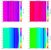 |
Fig. 4. Optimal/Limit steps histograms for Ωb (M1). Upper left panel: optimal steps for the 3-point derivatives; upper right panel: optimal steps for the 5-point derivatives; bottom left panel: critical steps for the 3-point derivatives; bottom right panel: critical steps for the 3-point derivatives. |
Figure 5 shows the optimal (upper panel) and the critical (bottom panel) step size for ln(H(1.35)) for the 3-point (left) and 5-point (right) stencil derivative. The optimal step size mainly lies around 10−6 for the 3-point stencil (even 1.5 × 10⁻⁷ in certain cells). The 5-point stencil mainly shows convergence from 10−5 to a few 10−4. Regarding the critical step size, here we took the truncation error as a limit because of its dominance when we compute derivatives over background quantities. The critical range for the 3-point derivatives extends from 10−1 to 10−4, while for the 5-point stencil, the range is 10−1 to a few 10−3. The lower bound of the critical range is one order of magnitude lower for the 5-point stencil. For the background quantities, taking low step sizes is a good option for computing accurate derivatives. The rounding errors remain much less dominant than the truncation errors.
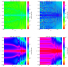 |
Fig. 5. Optimal/Limit steps histograms for ln(H(1.35)) (M2). Upper left panel: optimal steps for the 3-point derivatives; upper right panel: optimal steps for the 5-point derivatives; bottom left panel: critical steps for the 3-point derivatives; bottom right panel: critical steps for the 3-point derivatives. |
Ideally, it would be best to use an optimal step size for each value of the k and μ. However, from Figs. 4 and 5, we find that, when possible, a single step size should be selected, which will work efficiently over the whole parameter space. This single optimal step size should be below the critical value all over the parameter space. Tables 5 and 6 summarize the steps chosen for the M1 and M2 approaches using the 5-point method. For cosmological parameters, a step between 10−1 and 10−2 is enough to compute accurate derivatives. For background quantities, we use 10−4. We added the critical steps and hypercritical steps. The former corresponds to a choice of step size that ensures a precision on the derivatives better than the chosen level, while the latter is not expected to lead to the requested precision. The hypercritical steps are the same as the critical steps except for wa, whose step size is twice smaller (M1 approach) in order to increase the numerical noise; we also multiply, by a factor of 2, the steps of the background quantities (M2 approach) to increase the truncation errors. The constraints obtained by these 3 step cases are compared with the MCMC sampling.
Step values (approach M1): 5-point derivatives.
Step values (approach M2): 5-point derivatives.
4.3. Consistency: Approach M1 versus approach M2
In this section, we test the consistency of our results by comparing the two approaches, M1 and M2. This can be achieved by projecting the Fisher matrix from the M2 parameter space to the M1 parameter space. First, we consider the initial set of parameters given by the model M2 (these are: Pinitial[ωb, h, ωm, ns, ln(Da(0.125)), ln(H(0.125)), ln(fσ8(0.125)), ln(bσ8(0.125)), Pshot(0.125), …, ln(Da(2.55)), ln(H(2.55)), ln(fσ8(2.55)), ln(bσ8(2.55)), Pshot(2.55)]) and the final set of parameters (model M1), that is Pfinal[Ωb, h, Ωm, ns, ΩDE, w0, wa, σ8, ln(bσ8(0.125)), Pshot(0.125), …, ln(bσ8(2.55)), Pshot(2.55)]. We can project the initial Fisher matrix to the final one by simply using the chain rule (Wang 2006; Wang et al. 2010). The marginalization over the nuisance parameters can be done before or after the projection. In the latter case, they have to be taken into account during the projection:
 (9)
(9)
where indices i and j run over all unique pairs of parameters corresponding to the final model (we build the other half of the final Fisher matrix by computing the symmetric by mirroring over the diagonal). Indices α and β run over all parameter pairs corresponding to the M1 approach. We summarize the constraints relative errors obtained from the comparison between the standard M1 approach computation against the constraints after projection from the parameters introduced in the M2 approach in Table 7. Both covariances are marginalized over the nuisance parameters. We find that the two methods are in very good agreement, with the relative errors not exceeding ∼0.02%. The corresponding contours are shown in Fig. 6. As we can see, they are nearly perfectly superimposed. Therefore, the final Fisher matrices are highly consistent in the two approaches.
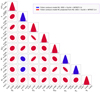 |
Fig. 6. Fisher approach M1 (blue) contours with optimal step sizes vs. Fisher approach M1 (red) with optimal step sizes contours projected from the model M2. Smaller contours are set in front. Here, the contours are nearly identical, with minor numerical differences putting one contour in front of the other nearly randomly. |
Relative errors on the cosmological parameter constraints between the M1 and M2 approaches (both with optimal step sizes) after projection to the θcosmo parameter set.
4.4. Fisher matrix and MCMC comparison
The relative errors between the MCMC and the Fisher constraints are presented in Tables 8 and 9. With the optimal steps, the relative error is lower than 5.5% for both models. With the critical steps, the wa relative error exceeds 10% (model M1). The other parameters have errors ranging from 2 × 10⁻³ to ∼6%. In the second approach, every step agrees well with the MCMC with the highest relative error of 9.118%. Choosing hypercritical steps leads to significant disagreement with the MCMC constraints. In the M1 approach, three cosmological parameters (ΩDE, w0 and wa) and one nuisance parameter (ln(bσ8(0.375))) do not fulfill the 10% agreement requirement level. The relative error on wa reaches 34%. In the M2 approach, the results are even worse, with most of the parameters having errors above 50%. Figures 7 and 8 show the Fisher contours using the optimal, critical, and hypercritical steps set. The covariances are marginalized over the nuisance parameters. For convenience, we only show the cosmological parameters for the M1 approach, and the cosmological as well as one redshift bin (z = 1.35) for the approach M2. In the M1 approach, as seen in Fig. 7, the Ωb, h, Ωm, ns and σ8 constraints are very stable for the 3-step set. The ΩDE parameter shows a slight difference between the 3-step set. The dark energy parameters, w0 and wa, show more appreciable differences, especially wa. In the M2 approach (Fig. 8) we can only see a few differences between the optimal and the critical steps set. However, the set of hypercritical steps gives very different results on all parameters except ns and Pshot(z)). The constraints are heavily overestimated (the uncertainties are too small) and fill around one third of the two other surface contours. We emphasize here that the only difference between the critical steps and the hypercritical steps is a factor of 2 on the steps for only one parameter in the M1 approach and two parameters on the M2 approach. The transition from the stable derivatives to the unstable derivatives is very sharp.
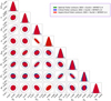 |
Fig. 7. Fisher contours: M1 approach, for the optimal (green), critical (blue), and hypercritical (red) steps. The contours are significantly affected when using an inappropriate step size, although the 1D likelihoods remain pretty stable. |
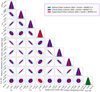 |
Fig. 8. Fisher contours: M2 approach, for the optimal (green), critical (blue), and hypercritical (red) steps. In this case, the use of critical step size leads to contours close the ones obtained with the optimal step size, while the hypercritical (twice the critical one) leads most of the contours to be incorrect, as well as most of the 1D likelihood. |
Checking the Fisher matrix derived constraints against the MCMC can give valuable information regarding the precision of the Fisher matrix estimation. However, this is not enough to validate the full procedure. Indeed, two multi-dimensional inference methods can result in the same constraints for each individual parameter, but with a different contour orientation. In order to ensure that this is not the case, the full posterior distribution has to be compared so we may check that all the contours orientations are similar. Figures 9 and 10 present the MCMC posterior distributions against the Fisher matrix ones (red lines) using the optimal steps settings. All the Fisher contours have the same orientation as the MCMC contours. Thus, the full procedure is validated. It is important to note that, fortunately, using one optimal step for all (k, μ, z) values is sufficient to have a very good level of agreement with the MCMC. That is to say, no adaptive derivatives approach is required. Moreover, the main differences between the Fisher and the MCMC contours come from slight non-Gaussianities on the posterior distribution. On some likelihood histograms in Figs. 9 and 10 we can see that the posterior from the MCMC follows “perfectly” one side of the Fisher, but not the other one (for instance, h in the M1 approach). This feature is less visible in the M2 approach likely due to the high number of accepted points in the MCMC chain, but it is still there, for example, in the case of ns.
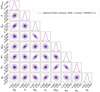 |
Fig. 9. MCMC vs Fisher optimal (red) contours: model M1. |
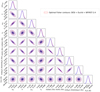 |
Fig. 10. MCMC vs Fisher optimal (red) contours: approach M2. |
MCMC vs Fisher relative errors (in percentage) for the model M1.
MCMC vs Fisher relative errors (in percentage) for the M2 approach.
5. Conclusions
In this paper, we investigate how to perform a comprehensive and robust validation of Fisher matrix forecasts by using a combination of three Stage IV spectroscopic surveys. We built vibration matrices for two different approaches for a fiducial cosmological model: a non-flat ΛCDM extended model where the dark energy equation of state follows the CPL parameterization which has two free variables: w0 and wa. In the first approach (M1), the Fisher matrix is obtained directly for the cosmological parameters, while in the second approach (M2), the background quantities are varied independently from the shape parameters, resulting in a much larger matrix; the final constraints are projected on the same parameter space for both approaches. We also found that the larger Fisher matrix is globally more sensitive to perturbations (as reflected by its high condition number). For instance, the Hubble parameter, h, is two orders of magnitude more sensitive in the second approach.
We studied the stability of the numerical derivatives over the cosmological parameters and found that the truncation error is particularly small within the step ranges considered. Cosmological parameters remain stable in the step range from 1 × 10⁻¹ to 3 × 10⁻⁴. Lower step values increase the rounding errors and result in higher total errors. Taking “large” steps is the safest way to perform the derivatives with respect to the cosmological parameters. The background quantities behave differently. The rounding errors remain small in all the step ranges considered. However, steps larger than 1 × 10⁻² for a 5-point stencil derivative give unstable results. Taking “large” steps for the background quantities is not safe because the differentiated function can oscillate on a scale smaller than the step size; this is exactly what must be avoided when computing the numerical derivatives. The convergence tests with respect to the 7-point stencil derivatives are performing better for the 5-point stencil. The convergence is reached between one and two orders of magnitude before the 3-point stencil case, and similarly for the convergence level. The safe steps window range of the 5-point stencil is then wider.
A comparison with the MCMC sampling shows the efficiency of the Fisher formalism even with non-adaptive derivatives, at least in the case where the posterior distribution is close to Gaussian. Although the optimal steps change with k and μ, choosing a unique step size for all the parameters does not produce appreciably larger errors that would significantly alter the forecasts. Furthermore, we considered a 1000 × 1000 (k, μ) grid which, multiplied by the number of redshift bins, amounts to computing 107 derivatives per parameter. One of the reasons for the stability comes from the fact that the contribution of the large scales on the derivatives is very small compared to the small scales contribution. Thus, taking optimal steps from high k values remains the best option. We have also seen that the transition between stable and unstable contours is quite sharp. Changing a step size by a factor of 2 in the wrong direction can give unstable contours.
Identifying and explaining the derivatives behavior and the effects on the constraints is difficult without the tests presented in this work. Our strategy allows for a comprehensive and robust validation of the constraints derived from the Fisher matrix formalism through a numerical method.
See Appendix C for a summary of the main definitions relevant for this work.
Acknowledgments
S. C. is funded by MIUR through Rita Levi Montalcini project ‘PROMETHEUS – Probing and Relating Observables with Multi-wavelength Experiments To Help Enlightening the Universe’s Structure’. S. C. acknowledges support from the ‘Departments of Excellence 2018-2022’ Grant (L. 232/2016) awarded by the Italian Ministry of Education, University and Research (MIUR). K. M.’s part of this research was carried out at the Jet Propulsion Laboratory, California Institute of Technology, under a contract with the National Aeronautics and Space Administration (80NM0018D0004). I. T. acknowledges support from the Spanish Ministry of Science, Innovation and Universities through grant ESP2017-89838-C3-1-R, and the H2020 programme of the European Commission through Grant 776247. A. P. is a UK Research and Innovation Future Leaders Fellow, Grant MR/S016066/1. D. S. acknowledges financial support from the Fondecyt Regular project number 1200171.
References
- Abbott, T. M. C., Abdalla, F. B., Alarcon, A., et al. 2018, Phys. Rev. D, 98, 043526 [Google Scholar]
- Akeson, R., Armus, L., Bachelet, E., et al. 2019, ArXiv e-prints [arXiv:1902.05569] [Google Scholar]
- Alam, S., Ata, M., Bailey, S., et al. 2017, MNRAS, 470, 2617 [NASA ADS] [CrossRef] [Google Scholar]
- Albrecht, A., Bernstein, G., Cahn, R., et al. 2006, ArXiv e-prints [arXiv:astro-ph/0609591] [Google Scholar]
- Amendola, L., & Sellentin, E. 2016, MNRAS, 457, 1490 [Google Scholar]
- Amendola, L., Appleby, S., Avgoustidis, A., et al. 2018, Liv. Rev. Rel., 21, 2 [Google Scholar]
- Belsley, D. A., Kuh, E., & Welsch, R. E. 2005, Regression Diagnostics: Identifying Influential Data and Sources of Collinearity (John Wiley & Sons) [Google Scholar]
- Blake, C., Kazin, E. A., Beutler, F., et al. 2011, MNRAS, 418, 1707 [NASA ADS] [CrossRef] [MathSciNet] [Google Scholar]
- Brooks, S. P., & Gelman, A. 1998, J. Comput. Graph. Stat., 7, 434 [Google Scholar]
- Chevallier, M., & Polarski, D. 2001, Int. J. Mod. Phys. D, 10, 213 [NASA ADS] [CrossRef] [Google Scholar]
- Chisari, N. E., Alonso, D., Krause, E., et al. 2019, ApJS, 242, 2 [NASA ADS] [CrossRef] [Google Scholar]
- Coe, D. 2009, ArXiv e-prints [arXiv:0906.4123] [Google Scholar]
- Dawson, K. S., Schlegel, D. J., Ahn, C. P., et al. 2013, AJ, 145, 10 [Google Scholar]
- Dawson, K. S., Kneib, J.-P., Percival, W. J., et al. 2016, AJ, 151, 44 [Google Scholar]
- DESI Collaboration (Aghamousa, A., et al.) 2016, ArXiv e-prints [arXiv:1611.00036] [Google Scholar]
- Dore, O., Hirata, C., Wang, Y., et al. 2019, BAAS, 51, 341 [Google Scholar]
- Dunkley, J., Bucher, M., Ferreira, P. G., Moodley, K., & Skordis, C. 2005, MNRAS, 356, 925 [NASA ADS] [CrossRef] [Google Scholar]
- Eisenstein, D. J., & Hu, W. 1998, ApJ, 496, 605 [NASA ADS] [CrossRef] [Google Scholar]
- Eisenstein, D. J., & Hu, W. 1999, ApJ, 511, 5 [NASA ADS] [CrossRef] [Google Scholar]
- Euclid Collaboration (Blanchard, A., et al.) 2020, A&A, 642, A191 [CrossRef] [EDP Sciences] [Google Scholar]
- Gelman, A., & Rubin, D. B. 1992, Stat. Sci., 7, 457 [Google Scholar]
- Green, J., Schechter, P., Baltay, C., et al. 2011, ArXiv e-prints [arXiv:1108.1374] [Google Scholar]
- Ivezić, Ž., Kahn, S. M., Tyson, J. A., et al. 2019, ApJ, 873, 111 [NASA ADS] [CrossRef] [Google Scholar]
- Joachimi, B., & Taylor, A. N. 2011, MNRAS, 416, 1010 [NASA ADS] [CrossRef] [Google Scholar]
- Laureijs, R., Amiaux, J., Arduini, S., et al. 2011, ArXiv e-prints [arXiv:1110.3193] [Google Scholar]
- Lesgourgues, J. 2011, ArXiv e-prints [arXiv:1104.2932] [Google Scholar]
- Lewis, A., Challinor, A., & Lasenby, A. 2000, ApJ, 538, 473 [Google Scholar]
- Linder, E. V. 2003, Phys. Rev. Lett., 90, 091301 [Google Scholar]
- LSST Science Collaboration (Abell, P. A., et al.) 2009, ArXiv e-prints [arXiv:0912.0201] [Google Scholar]
- Metropolis, N., & Ulam, S. 1949, J. Am. Stat. Assoc., 44, 335 [Google Scholar]
- Percival, W. J., Baugh, C. M., Bland-Hawthorn, J., et al. 2001, MNRAS, 327, 1297 [NASA ADS] [CrossRef] [Google Scholar]
- Perlmutter, S., Aldering, G., Goldhaber, G., et al. 1999, ApJ, 517, 565 [NASA ADS] [CrossRef] [Google Scholar]
- Planck Collaboration VI. 2020, A&A, 641, A6 [NASA ADS] [CrossRef] [EDP Sciences] [Google Scholar]
- Riess, A. G., Filippenko, A. V., Challis, P., et al. 1998, AJ, 116, 1009 [NASA ADS] [CrossRef] [Google Scholar]
- Robert, C. P. 2015, ArXiv e-prints [arXiv:1504.01896] [Google Scholar]
- Sellentin, E. 2015, MNRAS, 453, 893 [Google Scholar]
- Sellentin, E., Quartin, M., & Amendola, L. 2014, MNRAS, 441, 1831 [NASA ADS] [CrossRef] [Google Scholar]
- Seo, H.-J., & Eisenstein, D. J. 2003, ApJ, 598, 720 [Google Scholar]
- Spergel, D., Gehrels, N., Breckinridge, J., et al. 2013, ArXiv e-prints [arXiv:1305.5422] [Google Scholar]
- Square Kilometre Array Cosmology Science Working Group (Bacon, D. J., et al.) 2020, PASA, 37, e007 [CrossRef] [Google Scholar]
- Tegmark, M. 1997, Phys. Rev. Lett., 79, 3806 [NASA ADS] [CrossRef] [Google Scholar]
- Tegmark, M., Hamilton, A. J. S., Strauss, M. A., Vogeley, M. S., & Szalay, A. S. 1998, ApJ, 499, 555 [NASA ADS] [CrossRef] [Google Scholar]
- Tutusaus, I., Lamine, B., Blanchard, A., et al. 2016, Phys. Rev. D, 94, 123515 [NASA ADS] [CrossRef] [Google Scholar]
- Wang, Y. 2006, ApJ, 647, 1 [NASA ADS] [CrossRef] [Google Scholar]
- Wang, Y., Percival, W., Cimatti, A., et al. 2010, MNRAS, 409, 737 [NASA ADS] [CrossRef] [Google Scholar]
- Wolz, L., Kilbinger, M., Weller, J., & Giannantonio, T. 2012, JCAP, 2012, 009 [Google Scholar]
Appendix A: The Metropolis-Hastings sampler
Here we describe the steps to sample the parameter space from the SpecSAF MCMC module:
-
We initialize each parameter at its fiducial value and compute the corresponding observed power spectrum (Eq. (4)).
-
We draw a new parameter set from a multivariate normal distribution (mean = current parameter set) and compute the new observed power spectrum. The multivariate normal distribution is the one given by the inverse of the Fisher matrix for the same specifications (i.e., the covariance matrix).
-
We perform a χ2 test in order to get the sum of the square errors:
 (A.1)
(A.1)with σp(k, μ, z) the errors of the logarithm of the observed power spectrum given by Seo & Eisenstein (2003):
 (A.2)
(A.2)with n(z) the mean density of galaxies at a given redshift bin.
-
We finally compute the likelihood ratio:
 (A.3)
(A.3) -
We draw a random number RN in the interval [0, 1] from a uniform distribution.
-
We compare LR and RN: – if LR ≥ RN the parameter set is accepted and the new parameter set is updated. – else the parameter set is not accepted and the new parameter set is not updated.
-
We loop over 2–6.
Finally we stop the chains using the Gelman-Rubin diagnostic, described in Appendix B.
Appendix B: The Gelman-Rubin diagnostic
The Gelman-Rubin diagnostic aims to monitor MCMC outputs for parallelized chains. The convergence test computes a constant, (R − 1), proportional to the ratio of the parameters variance of one chain to the mean parameters variances of the independent chains. The mean of the empirical variance within each chain W is defined as:
 (B.1)
(B.1)
with M the number of chains, P the number of parameters and N the number of accepted points for each chain;  represents the mean value drawn of a parameter α for one chain and
  the i-th α value drawn. The between-chain variance B is given by:
 (B.2)
(B.2)
The weighted sum of W and B is written as:
 (B.3)
(B.3)
Finally, the R number is defined as:
 (B.4)
(B.4)
with  the degrees of freedom estimate of a given distribution. The convergence is reached once (R − 1) < 0.03 “(i.e., R must be sufficiently close to 1)”. We provide the (R − 1) values obtained for the approaches M1 and M2 in Tables B.1 and B.2, respectively.
(R − 1) values for approach M1.
(R − 1) values for approach M2.
Appendix C: General definitions
In this last part of the appendix, we summarize the main definitions relevant for this work.
Optimal step. Step size providing the minimum relative error between the analytical form and the numerical solutions. It ensures the most accurate derivative.
Critical step. Step size that can potentially lead to an error of 10% on the final constraints.
Hypercritical step. Step size that can potentially lead to catastrophic errors (several dozen percent) on the final constraints.
Truncation error. Error introduced by considering too large step sizes. The approximation of computing the derivative with a finite amount of terms is in this case no longer valid.
Rounding error. Error introduced by considering too small step sizes. The finite precision floating point numbers used on computers cannot distinguish between numbers that are too close.
Vibration matrix. Matrix providing the largest value of the vibration for which 68% of the constraints on each parameter remain smaller than the chosen precision.
All Tables
Redshift range, binning choices, and density of galaxies for the surveys used in this work.
Fiducial values of the shape and redshift dependent parameters for the approach M2.
Relative errors on the cosmological parameter constraints between the M1 and M2 approaches (both with optimal step sizes) after projection to the θcosmo parameter set.
All Figures
|
Fig. 1. Vibration matrix: approach M1. The values are expressed in absolute values. Each cell containing 1 has to be taken as a lower bound value of the limit because we take 1 as the threshold perturbation amplitude. |
| In the text | |
|
Fig. 2. Vibration matrix: approach M2. We note that some values are identical because we decreased the resolution of the perturbation amplitude range. |
| In the text | |
|
Fig. 3. Stability and convergence tests towards the 7-point stencil for wa and ln(Da(1.35)) at a given k and μ at z = 1.35. Upper left panel: stability of wa; upper right panel: stability of ln(Da(1.35)); bottom left panel: convergence of ωm; bottom right panel: convergence of ln(Da(1.35)). Blue: 3-point stencil, red: 5-point stencil, green: 7-point stencil. |
| In the text | |
|
Fig. 4. Optimal/Limit steps histograms for Ωb (M1). Upper left panel: optimal steps for the 3-point derivatives; upper right panel: optimal steps for the 5-point derivatives; bottom left panel: critical steps for the 3-point derivatives; bottom right panel: critical steps for the 3-point derivatives. |
| In the text | |
|
Fig. 5. Optimal/Limit steps histograms for ln(H(1.35)) (M2). Upper left panel: optimal steps for the 3-point derivatives; upper right panel: optimal steps for the 5-point derivatives; bottom left panel: critical steps for the 3-point derivatives; bottom right panel: critical steps for the 3-point derivatives. |
| In the text | |
|
Fig. 6. Fisher approach M1 (blue) contours with optimal step sizes vs. Fisher approach M1 (red) with optimal step sizes contours projected from the model M2. Smaller contours are set in front. Here, the contours are nearly identical, with minor numerical differences putting one contour in front of the other nearly randomly. |
| In the text | |
|
Fig. 7. Fisher contours: M1 approach, for the optimal (green), critical (blue), and hypercritical (red) steps. The contours are significantly affected when using an inappropriate step size, although the 1D likelihoods remain pretty stable. |
| In the text | |
|
Fig. 8. Fisher contours: M2 approach, for the optimal (green), critical (blue), and hypercritical (red) steps. In this case, the use of critical step size leads to contours close the ones obtained with the optimal step size, while the hypercritical (twice the critical one) leads most of the contours to be incorrect, as well as most of the 1D likelihood. |
| In the text | |
|
Fig. 9. MCMC vs Fisher optimal (red) contours: model M1. |
| In the text | |
|
Fig. 10. MCMC vs Fisher optimal (red) contours: approach M2. |
| In the text | |
Current usage metrics show cumulative count of Article Views (full-text article views including HTML views, PDF and ePub downloads, according to the available data) and Abstracts Views on Vision4Press platform.
Data correspond to usage on the plateform after 2015. The current usage metrics is available 48-96 hours after online publication and is updated daily on week days.
Initial download of the metrics may take a while.