© ESO 2021

1. Introduction

Stitching an accretion disk rotating at about the Keplerian rate with the central object rotating much more slowly leads to the concept of the accretion boundary layer (BL). The reason for talking about the BL as an entity separate from the accretion disk is the inevitable breakdown of the basic assumptions of the standard disk theory in a very narrow region just above the surface of the accretor (Lynden-Bell & Pringle 1974; Papaloizou & Stanley 1986).

In neutron star (NS) low-mass X-ray binaries (LMXBs), the BL is thought to be an important source of radiation when the magnetic field of an accreting NS is too weak to support a magnetosphere. Shining at a luminosity comparable to that of the accretion disk (Lynden-Bell & Pringle 1974; Sibgatullin & Sunyaev 2000), but being much more compact, the BL is expected to have a harder spectrum and shorter variability time scales. Such a component has indeed been identified in LMXBs, spectrally (Suleimanov & Poutanen 2006; Revnivtsev et al. 2013) and via its timing properties, in particular as a source of kilohertz quasi-periodic oscillations (kHz QPOs; Gilfanov et al. 2003). The position of the BL at the surface of the NS makes it a valuable probe for the fundamental properties of the star: its size, radius, and the physical conditions on its surface.

The kHz QPOs have been observed in many NS LMXBs (van der Klis 2000). Their frequencies span the range between about 200 Hz and the Keplerian frequency near the surface (about 1.3 kHz; see Méndez et al. 1999; Belloni et al. 2005). Either one or two peaks, with a frequency difference of about 300 Hz (Méndez & Belloni 2007), are observed. In individual sources, kHz QPO frequencies may vary by a factor of 1.5–2. The frequencies are correlated with flux on time scales of hours (Méndez et al. 1999, 2001), while the correlation disappears on time scales of days. This phenomenon, known as QPO parallel tracks, was explained in a purely phenomenological way by van der Klis (2001). He suggested that the instantaneous X-ray luminosity of the source is a linear combination of the mass accretion rate Ṁ and its running average ⟨Ṁ⟩, while the oscillation frequency is a function of Ṁ/⟨Ṁ⟩ only. In this paper, we propose a mathematically similar but more physically motivated solution to the parallel tracks problem.

We have developed a simple mechanical model of the BL, which is treated as a thin massive belt supplied by the mass and angular momentum from the accretion disk and which is losing mass and angular momentum to the NS. We consider the rotation frequency of the BL to be the characteristic frequency responsible for kHz QPOs, though the real situation is probably much more complicated (e.g., Abolmasov et al. 2020). In Sect. 2, we introduce the main equations based on conservation laws. In Sect. 3, we consider the properties of the model by solving the equations numerically. We discuss the results in Sect. 4.

2. Model setup

We consider the BL as an infinitely thin equatorial belt on the surface of a NS of radius R and mass M_NS rotating at an angular frequency Ω_NS. The rotation of the layer is aligned with both the rotation of the star and the disk. The dynamics of the layer can be reduced to two equations, one for the mass and the other for the angular momentum conservation. The conservation law for the BL mass M can be written as

$$\begin{array}{c}\hfill \frac{\mathrm{d}M}{\mathrm{d}t}=\dot{M}-\frac{M}{t_{\mathrm{depl}}},\end{array}$$(1)

where Ṁ is the mass supply rate from the disk. The second term describes mass precipitation from the BL onto the NS surface with the depletion time scale t_depl that exceeds the characteristic dynamical (Keplerian) time scale $t_{\mathrm{dyn}}=1/{\mathrm{\Omega }}_{\mathrm{K}}=\sqrt{R^3/G{M}_{\mathrm{NS}}}$, where Ω_K is the Keplerian frequency.

Conservation of the angular momentum also involves sources and sinks related to the interaction with the surface of the star. Hydrodynamic numerical simulations (e.g., Belyaev et al. 2013) suggest that the interaction between the BL and the surface of the star mediated by Reynolds stress is relatively weak. The relevant tangential stress W_rφ ∼ 10⁻⁶P, where P is the pressure at the bottom of the layer. The impact of magnetic fields on the internal dynamics of the layer is probably important (Armitage 2002), but it is unclear if they can provide an efficient angular momentum transfer between the BL and the star. We will assume that the stress at the bottom of the BL is proportional to the pressure with a small proportionality coefficient α ≪ 1,

$$\begin{array}{c}\hfill W_{r\phi }=\alpha P=\alpha g_{\mathrm{eff}}\mathrm{\Sigma },\end{array}$$(2)

where Σ is the BL surface density and

$$\begin{array}{c}\hfill g_{\mathrm{eff}}=\frac{G{M}_{\mathrm{NS}}}{R^2}-{\mathrm{\Omega }}^{2}R\end{array}$$(3)

is the effective surface gravity, where Ω is the rotation frequency of the layer. This allows us to express the braking torque acting on the layer as

$$\begin{array}{c}\hfill T^{-}=AR{W}_{r\phi }=\alpha g_{\mathrm{eff}}MR,\end{array}$$(4)

where A is the surface area of the BL (projected onto the surface of the star) and the BL mass is M = AΣ.

The angular momentum conservation law that includes mass depletion and friction takes the form

$$\begin{array}{c}\hfill \frac{\mathrm{d}J}{\mathrm{d}t}=\dot{M}{j}_{\mathrm{d}}-\frac{J}{t_{\mathrm{depl}}}-\alpha g_{\mathrm{eff}}MR,\end{array}$$(5)

where J = ΩMR² is the total angular momentum of the layer and $j_{\mathrm{d}}=\sqrt{G{M}_{\mathrm{NS}}R}$ is the specific angular momentum of the matter entering from the disk. We ignore viscous interaction between the disk and the BL. This corresponds to the “accretion gap” scenario (Kluzniak & Wagoner 1985), where the last stable orbit is located above the surface of the NS and thus the disk is causally disconnected from the BL. Recent constraints for the NS radius (Nättilä et al. 2017; Miller et al. 2019; Riley et al. 2019; Capano et al. 2020) suggest that this should be the case, at least below the Eddington limit.

Two equations, Eqs. (1) and (5), are sufficient to describe the evolution of the physical parameters of the BL with time, given Ṁ(t) and initial conditions. In our framework, the energy released during accretion and dissipation does not affect the dynamics of the layer. However, luminosity is an important observable. Some of the kinetic energy of the flow contributes to the spin-up of the star; the rest is converted to heat and contributes to the luminosity. The dissipated luminosity can be found as the change in the kinetic energy (see, e.g., Appendix B of Popham & Narayan 1995). Our model splits this spin-down of the gas being accreted into two episodes: Some dissipation occurs when the matter from the disk enters the BL at the rate Ṁ, and some dissipation occurs during the matter depletion from the BL (at the rate of M/t_depl). In addition to these two components, there is viscous dissipation unrelated to mass exchange, equal to one-half of the stress W_rφ times the strain RdΩ/dR (see Landau & Lifshitz 1987, section 16). Together, the luminosity associated with the BL can be written as the sum of three terms:

$$\begin{array}{cc}\hfill {\displaystyle L}& {\displaystyle =\frac{1}{2}\dot{M}{R}^2({\mathrm{\Omega }}_{\mathrm{d}}^2-{\mathrm{\Omega }}^2)+\frac{1}{2}\alpha g_{\mathrm{eff}}MR(\mathrm{\Omega }-{\mathrm{\Omega }}_{\mathrm{NS}})}\hfill \\ \hfill & +\frac{1}{2}\frac{M}{t_{\mathrm{depl}}}{R}^2({\mathrm{\Omega }}^2-{\mathrm{\Omega }}_{\mathrm{NS}}^2).\hfill \end{array}$$(6)

The first term on the right-hand side is the kinetic energy lost by the matter that enters the BL from the disk with the angular frequency Ω_d = j_d/R². The second term is the viscous dissipation associated with the Reynolds stress (Eq. (2)). The last term corresponds to the kinetic energy of the BL material that precipitates onto the NS and acquires its rotation velocity.

Below, we assume that the BL is fed by a variable source of mass. We assume stochastic variability of the mass accretion rate, modeled as a white noise source convolved with a kernel corresponding to a power-law power-density spectrum (PDS) with a random Fourier image phase (which corresponds to a random moment in time and unsynchronized variability at different frequencies). Integrating white noise leads to a normally distributed quantity as it involves the summation of a large number of independent random numbers. To reproduce the log-normal flux distribution reported in many observational works (Uttley et al. 2005), we then exponentiated the result of the convolution and renormalized it to match the mean value of Ṁ.

3. Results

3.1. Approach to the equilibrium solution

For a fixed BL mass and mass accretion rate, the rotation of the BL can be described as evolution toward an equilibrium state. Using Eqs. (1) and (5), we can derive an evolutionary equation for Ω:

$$\begin{array}{cc}\hfill {\displaystyle \frac{\mathrm{d}\mathrm{\Omega }}{\mathrm{d}t}}& =\frac{\mathrm{d}}{\mathrm{d}t}\left(\frac{J}{M{R}^2}\right)=\frac{J}{M{R}^2}(\frac{\dot{M}{j}_{\mathrm{d}}}{J}-\frac{\dot{M}}{M}-\frac{\alpha g_{\mathrm{eff}}MR}{J})\hfill \\ \hfill {\displaystyle }& =\frac{\dot{M}}{M}({\mathrm{\Omega }}_{\mathrm{d}}-\mathrm{\Omega })-\alpha ({\mathrm{\Omega }}_{\mathrm{K}}^2-{\mathrm{\Omega }}^2).\hfill \end{array}$$(7)

The right-hand side of this equation is quadratic in Ω, which allows us to rewrite it in the form

$$\begin{array}{c}\hfill \frac{\mathrm{d}\mathrm{\Omega }}{\mathrm{d}t}=\alpha ({\mathrm{\Omega }}_{-}-\mathrm{\Omega })({\mathrm{\Omega }}_{+}-\mathrm{\Omega }),\end{array}$$(8)

where

$$\begin{array}{c}\hfill {\mathrm{\Omega }}_{\pm }=\frac{\dot{M}}{2\alpha M}\pm \sqrt{{(\frac{\dot{M}}{2\alpha M}-{\mathrm{\Omega }}_{\mathrm{K}})}^2+\frac{\dot{M}}{\alpha M}({\mathrm{\Omega }}_{\mathrm{K}}-{\mathrm{\Omega }}_{\mathrm{d}})}.\end{array}$$(9)

For Ω_d = Ω_K, one of the frequencies becomes Ω₊ = Ω_K and the other Ω₋ = Ṁ/(αM) − Ω_K. The lower of the two roots, which is always Ω₋ for the parameter values we consider (see Sect. 3.3 for more details), is stable.

Our approximation is valid only if Ω < Ω_K; otherwise, effective gravity becomes negative and the flow is unbound. Unless Ω₋ becomes smaller than Ω_NS, the BL will evolve toward this equilibrium state. Otherwise, the layer stalls at Ω = Ω_NS, and W_rφ works as static friction.

At a fixed mass accretion rate, the system reaches both equilibrium mass and equilibrium rotation frequency. Mass equilibrium is given by

$$\begin{array}{c}\hfill M=M_{\mathrm{eq}}=\dot{M}{t}_{\mathrm{depl}}.\end{array}$$(10)

The equilibrium rotation frequency depends on the ratio Ω_d/Ω_K, which we fix to 1, and on only one additional parameter αM_eq/Ṁ. It is easy to check that this quantity, multiplied by the Keplerian frequency, is equal to the ratio of the characteristic depletion and friction time scales,

$$\begin{array}{c}\hfill q=\frac{t_{\mathrm{depl}}}{t_{\mathrm{fric}}}=\alpha {\mathrm{\Omega }}_{\mathrm{K}}{t}_{\mathrm{depl}}.\end{array}$$(11)

For Ω_d = Ω_K, the equilibrium rotation frequency is

$$\begin{array}{c}\hfill {\mathrm{\Omega }}_{\mathrm{eq}}=(\frac{1}{q}-1){\mathrm{\Omega }}_{\mathrm{K}}.\end{array}$$(12)

When the friction becomes more efficient than depletion, the layer brakes down to Ω = Ω_NS, which leads to trivial rotational evolution. Hence, in the simulations with the variable mass accretion rate, we keep α ≲ 1/(Ω_Kt_depl).

3.2. Variable mass accretion rate

If the mass accretion inflow to the layer is variable, the BL works as a filter for the variability of Ṁ. The system of equations we consider is practically linear, though there is nonlinearity introduced by g_eff in the friction term in Eq. (5). The characteristic depletion and friction time scales are presumably much longer than the dynamical time, and they probably also exceed the viscous time scales in the inner disk. The outer disk, however, evolves even more slowly. In the relevant frequency range, the shapes of the PDSs of LMXBs are generally close to a power-law PDS ∝ f^−p with a slope of p ≃ 1.3 (Gilfanov & Arefiev 2005). We used this spectral slope in our simulations as representative of the variability of the disk.

The mean mass accretion rate was set to Eddington Ṁ = L_Edd/c². The exact value does not affect the qualitative picture of accretion but sets the accretion time scale and equilibrium mass of the layer. As mentioned in Sect. 2, the variations of the mass accretion rate logarithm were considered as an integral of a white noise process. This allowed us to introduce one extra parameter, the dispersion of ln Ṁ. In our simulations, we set the root-mean-square deviation of the mass accretion rate logarithm $D=\sqrt{\langle {(\mathrm{\Delta }ln\dot{M})}^2\rangle }$ to 0.5. This value allows us to reproduce the relative variations of the characteristic frequencies without strong inconsistency with the flux variation amplitudes in LMXBs (Hasinger & van der Klis 1989; Méndez et al. 1999).

In our model, the BL does not have any variability of its own, and hence the variations of its luminosity are essentially smaller than that of the mass accretion rate, especially at high frequencies. In reality, of course, there is an additional variability component originating in the layer. The BL light curve is smoother and lags the mass accretion rate, as one would expect from the properties of the model where the BL emission depends on the history of the mass accretion rate.

We computed the cross-spectra of BL luminosity, L (see Eq. (6)), and its rotation frequency, Ω, which are the proxies for the flux and QPO frequency, respectively. The argument of the cross-spectrum gives the phase lags, which we show in Fig. 1 as a function of Fourier frequency. We also computed the coherence (Vaughan & Nowak 1997; Nowak et al. 1999) shown in the lower panel of the figure. Both are averaged over a series of 10⁴ light curves.

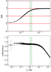Fig. 1. Phase lags (upper panel) and coherence (lower panel) between the instantaneous luminosity of the BL, L, and its rotation frequency, Ω. A positive phase lag means that Ω lags L. The vertical green lines show the frequencies corresponding to the depletion tdepl (dot-dashed) and the friction 1/αΩK (dashed) time scales. Additional error bars (vertical dotted black lines) show the variability of the quantities within the bin. The parameters are α = 10−7, tdepl ≃ 740 s (corresponding to q ≃ 0.68), and a NS spin period of 3 ms.

Quite expectedly, the quantities are correlated at lower frequencies but uncorrelated at f ≫ 1/t_{depl,  fric}. Maximal coherence, however, occurs at intermediate frequencies, f ∼ (0.1−1)/t_{depl,  fric}. At higher frequencies, luminosity becomes sensitive to rapid variations in Ṁ that are uncorrelated with Ω. Phase lags at low frequencies are negative as the variations of L lag the variations of Ṁ, while Ω follows the variations of Ω⁻(Ṁ, M) (see Sect. 3.3). The phase lags increase with frequency and become positive at time scales that are somewhat longer than the time scales of the BL (∼t_depl and t_fric). At high frequencies, they approach Δφ = π/2. Such a flat phase lag spectrum is a natural outcome of the mathematical properties of the initial system of equations. The luminosity given by Eq. (6) contains one term proportional to Ṁ (the first term, related to the variable mass inflow to the BL). The other two terms depend only on M = ∫Ṁdt + const and on Ω. The spectral slope of Ṁ is always shallower than that of M. At a given frequency f, the friction and depletion terms have contributions of ∼1/(ft_{fric,  depl}) with respect to the first term. Thus, at high frequencies, the variability of L is dominated by variations in the mass accretion rate. Rotation frequency at high f (when M ≃ const) is a result of the integration of Ω₋ (see Eq. (9)), which is a function of Ṁ and M. Taking the Fourier transform of Eq. (8) in the high-frequency limit yields

$$\begin{array}{c}\hfill 2\mathrm{\pi }\mathrm{i}f\stackrel{\sim }{\mathrm{\Omega }}\simeq ({\mathrm{\Omega }}_{\mathrm{K}}-\mathrm{\Omega })\frac{\stackrel{\sim }{\dot{M}}}{M},\end{array}$$(13)

where all the higher-order terms in f are neglected, Ω₊ is replaced with Ω_K, and the Fourier transform of Ω₋ is replaced by $\stackrel{\sim }{\dot{M}}/\alpha M$. Hence, in this limit, the Fourier image of the rotation frequency is

$$\begin{array}{c}\hfill \stackrel{\sim }{\mathrm{\Omega }}\simeq \frac{1}{2\mathrm{\pi }if}\frac{\stackrel{\sim }{\dot{M}}}{M}({\mathrm{\Omega }}_{\mathrm{K}}-\mathrm{\Omega }).\end{array}$$(14)

As L is mainly affected by the first term, the cross-spectrum becomes

$$\begin{array}{cc}\hfill {\displaystyle C(L,\mathrm{\Omega })}& \simeq \frac{1}{2}{R}^2({\mathrm{\Omega }}_{\mathrm{K}}^2-{\mathrm{\Omega }}^2)\stackrel{\sim }{\dot{M}}{\stackrel{\sim }{\mathrm{\Omega }}}^{\ast }\hfill \\ \hfill {\displaystyle }& \simeq \frac{\mathrm{i}}{4\mathrm{\pi }f}{R}^2({\mathrm{\Omega }}_{\mathrm{K}}^2-{\mathrm{\Omega }}^2)({\mathrm{\Omega }}_{\mathrm{K}}-\mathrm{\Omega }){\left|{\stackrel{\sim }{\dot{M}}}^{\ast }\right|}^2.\hfill \end{array}$$(15)

The argument of this expression is π/2.

3.3. Rotation frequency variations

The behavior of the BL, including its rotation frequency, depends strongly on the balance between mass and angular momentum loss, which can be described by the dimensionless quantity q (see Eq. (11)). In Fig. 2, we show the mean rotation frequency and its variations for different values of q. Apparently, the mean value is well predicted by the Ω₋ given by Eq. (9). When the depletion time scale is much shorter (q ≲ 0.5), the BL corotates with the disk. In the opposite limit, friction spins the BL down to Ω_NS. Strong variations in Ω are present only when the two time scales (friction and depletion) are comparable (q ≃ 0.5−0.9).

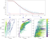Fig. 2. Rotation frequency dependence on q and luminosity. Upper panel: mean BL rotation frequency (black dots; error bars show the root-mean-square variations of Ω) as a function of q compared to the equilibrium value, Ω− (solid red line). The dashed red line shows the rotation frequency of the NS (3 ms). Lower panels: BL rotation frequency dependence on instantaneous luminosity for sample light curves with three different values of depletion time corresponding to q = 0.4, 0.6, and 0.8. In all the simulations, α = 10−7. Time in the lower panels is color-coded (see the colorbar on the right). The crosses are the average values calculated for 64 s time bins, and the error bars show the standard deviation.

In general, the relation between the observed luminosity and rotation frequency of the layer is nonunique, and the parallel tracks picture is qualitatively reproduced (see the lower panels of Fig. 2). On the shortest time scales, much smaller than t_{depl,  fric}, the variability of the luminosity is dominated by the first term in Eq. (6), which is uncorrelated with Ω. However, if the luminosity is averaged in time bins that are several times smaller than the time scales of the BL, it becomes correlated with Ω. On these time scales, the variations of Ω₋ in Eq. (8) dominate over the variations of Ω (see Fig. 3), hence the rotation frequency derivative

$$\begin{array}{c}\hfill \frac{\mathrm{d}\mathrm{\Omega }}{\mathrm{d}t}\simeq ({\mathrm{\Omega }}_{\mathrm{K}}-\mathrm{\Omega })\frac{\dot{M}}{M}.\end{array}$$(16)

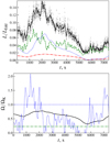Fig. 3. Luminosity and frequency variations with time. Upper panel: portion of the light curve of the simulation with α = 10−7 and q = 0.6. The solid black curve shows the total 64-second-averaged luminosity (Eq. 6). We also show three contributions to the luminosity separately: The first, second, and third terms from Eq. (6) are plotted with dashed green, dotted blue, and dot-dashed red lines, respectively. The black dots are instantaneous luminosity values (every 2 s). Lower panel: rotation frequency Ω (solid black line) and Ω± (dotted blue lines) for the same model. The horizontal dashed green line corresponds to the spin of the NS.

Neglecting mass depletion, this yields

$$\begin{array}{c}\hfill M\propto \frac{1}{{\mathrm{\Omega }}_{\mathrm{K}}-\mathrm{\Omega }},\end{array}$$(17)

where the proportionality coefficient is a slowly variable function of time. This scaling is well reproduced in the evolution of the BL on time scales that are several times smaller than the friction and depletion scales (Fig. 4). Luminosity variations also follow a similar trend, L ∝ (Ω_K−Ω)⁻¹.

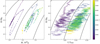Fig. 4. Parallel tracks on the M − Ω and L − Ω planes for a simulation with α = 10−7, q = 0.56, D = 0.5, and p = 1.3. Solid black lines are the lines of (ΩK−Ω)M = const and (ΩK−Ω)L=const. Time is color-coded (see the colorbar on the right). To demonstrate the parallel tracks effect during multiple observation runs, we show only the data points in 104 s intervals separated by 104 s gaps.

3.4. The influence of the other model parameters

Despite its simplicity, the model has several parameters, the values of which are not derived from the basic principles. The influence of the rotation frequency of the star Ω_NS does not change the overall behavior. For the solutions with q ≲ 1, it only limits the possible values of Ω and slightly modulates the spin-down term. The mean mass accretion rate in the framework of our model also plays a secondary role, affecting only the luminosity of the BL.

The variability spectrum of the mass accretion rate is encoded by two parameters, the root-mean-square variation of the mass accretion rate logarithm D and the slope of the power-law spectrum p. Their influence on the parallel tracks effect is shown in Figs. 5 and 6. A redder variability spectrum allows the system to accrete longer at a steady rate that is different from the mean value and thus increases the variations of mass and angular momentum. Thus, the parallel tracks effect is much more prominent for the case of red noise (right-hand panel of Fig. 5). A harder variability spectrum (p ≲ 1) makes the parallel tracks closer. However, the L ∝ (Ω_K−Ω)⁻¹ scaling still holds well.

Fig. 5. Same as the right-hand panel of Fig. 4 but for p = 1 (left panel) and p = 2 (right panel).

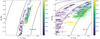Fig. 6. Same as the right-hand panel of Fig. 4 but for D = 0.25 (left panel) and D = 1 (right panel).

Different values of D (see Fig. 6) also affect the prominence of the parallel tracks effect. As the amplitude of the mass accretion rate variations increases by a factor of several, the spacing between the short-term tracks increases from about 30% to nearly two orders of magnitude.

4. Discussion

4.1. Friction and depletion times

As mentioned in the introduction, the observed kHz QPO frequencies vary by a factor of 1.5–2 in individual sources. While our model reproduces the parallel tracks effect in a broad range of parameters, strong variations in the rotation frequency of the BL appear only when the characteristic friction and mass depletion time scales are comparable. If friction is more efficient (q ≳ 0.8), the BL corotates with the star. If depletion is faster (q ≲ 0.5), the BL corotates with the disk and loses angular momentum only with mass. Effectively, the second independent parameter necessary to reproduce the parallel tracks behavior exists only in a narrow range of q, meaning that there should be a physical reason for the depletion and friction time scales to be close to each other.

Such a similarity in the time scales may be explained if the BL is resolved in the radial direction. The radial flux of angular momentum consists of two parts, viscous w_rφR and advective ωR²ρv, where v is vertical velocity, h ≪ R is the height above the NS surface, w_rφ = w_rφ(h) is the viscous stress component, and ω = ω(h) is the rotation frequency, decreasing from Ω somewhere inside the BL to Ω_NS at the NS surface. Because the viscous angular momentum transfer is directed outward in the disk and inward at the bottom of the BL, at some altitude it should be zero. Let us assume that w_rφ = 0 at the same altitude where ω = Ω, and describe the angular momentum transfer along the radial coordinate by the following equation

$$\begin{array}{c}\hfill \frac{\partial }{\partial t}\left(\omega R^2\right)+v\frac{\partial }{\partial h}\left(\omega R^2\right)=-\frac{1}{R\rho }\frac{\partial }{\partial h}\left(w_{r\phi }{R}^2\right).\end{array}$$(18)

In a steady-state case, ρv = const and the time derivative in Eq. (18) is zero. Integration yields

$$\begin{array}{c}\hfill \rho v\omega R^2+w_{r\phi }R=\rho v\mathrm{\Omega }{R}^2.\end{array}$$(19)

At the surface of the NS, ω(h) = Ω_NS and w_rφ = W_rφ, which implies

$$\begin{array}{c}\hfill \rho v(\mathrm{\Omega }-{\mathrm{\Omega }}_{\mathrm{NS}})R^2=R{W}_{r\phi }.\end{array}$$(20)

Multiplying this equation by A and taking Eq. (4) into account yields

$$\begin{array}{c}\hfill \frac{M}{t_{\mathrm{depl}}}(\mathrm{\Omega }-{\mathrm{\Omega }}_{\mathrm{NS}})R^2=\alpha g_{\mathrm{eff}}MR.\end{array}$$(21)

We note that the mass flux ρv is related to the mass motion from the BL onto the surface of the star, and hence we replaced ρvA with M/t_depl. Substituting g_eff from Eq. (3), we can express the q parameter using Eq. (11) as

$$\begin{array}{c}\hfill q=\frac{{\mathrm{\Omega }}_{\mathrm{K}}(\mathrm{\Omega }-{\mathrm{\Omega }}_{\mathrm{NS}})}{{\mathrm{\Omega }}_{\mathrm{K}}^2-{\mathrm{\Omega }}^2}.\end{array}$$(22)

These estimates suggest that, instead of being an independent parameter, q should depend on the rotation frequency of the BL. It is unclear if q should change with the variations of Ω. If q depends on the mean or instantaneous value of Ω, Eq. (12) predicts an attractor for Ω/Ω_K and q. Combining Eqs. (12) and (22), we get

$$\begin{array}{c}\hfill {\displaystyle q=\frac{2}{3+{\mathrm{\Omega }}_{\mathrm{NS}}/{\mathrm{\Omega }}_{\mathrm{K}}},}\end{array}$$(23)

and for the equilibrium rotation frequency we obtain

$$\begin{array}{c}\hfill {\mathrm{\Omega }}_{\mathrm{eq}}=\frac{{\mathrm{\Omega }}_{\mathrm{K}}+{\mathrm{\Omega }}_{\mathrm{NS}}}{2}.\end{array}$$(24)

In Fig. 7, we show how our dynamical model behaves if the depletion time depends on rotation frequency as $t_{\text{depl}}=\left(\mathrm{\Omega }-{\mathrm{\Omega }}_{\text{NS}}\right)/\alpha \left({\mathrm{\Omega }}_{\text{K}}^2-{\mathrm{\Omega }}^2\right)$ for a fixed value of α, which implies q following Eq. (22). The parallel tracks effect is still reproduced in this version of the model.

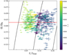Fig. 7. Same as the right-hand panel of Fig. 4 but for a model with α = 10−7 and q given by Eq. (22). The horizontal red line corresponds to the Ωeq given by Eq. (24)

4.2. Observable frequencies

Here, we consider the rotation frequency of the BL as a characteristic QPO frequency. Though this is probably not the case, the real dynamical processes behind kHz QPOs are still likely sensitive to Ω. If the real oscillation frequencies are functions of Ω and L or M, the parallel tracks effect is equally well reproduced, though the parameters of the correlation with radiation flux change.

In particular, for the Rossby-wave model considered in Abolmasov et al. (2020), the characteristic oscillation frequencies are the epicyclic frequency

$$\begin{array}{c}\hfill {\mathrm{\Omega }}_{\mathrm{e}}\simeq 2\mathrm{\Omega }cos\theta ,\end{array}$$(25)

where θ is the colatitude of the region where the oscillations are excited as well as its aliases with rotation frequency Ω_e + nΩ, where n is a whole number. The oscillations are likely excited in the region of strongest latitudinal velocity shear, which is unstable to supersonic shear instability. This naturally explains the multiplicity of kHz QPO frequencies and the difference between the frequencies that tends to be close to Ω_NS (though not necessarily; see Méndez et al. 2001). Such a model also explains the characteristic values of the QPO frequencies and their correlation with the flux (cos θ is likely a growing function of L; see Inogamov & Sunyaev 1999; Suleimanov & Poutanen 2006), as well as the different quality factors of the two QPO peaks (quality factors of the axisymmetric mode n = 0 and all others should differ since visibility effects enhance the periodic component in a non-axisymmetric case). It is unclear, however, how to explain the existence of only two QPO peaks (probably n = 0 and −1). Higher harmonics may be below the sensitivity level, or their excitation conditions may be different. If, instead of rotation frequency, we plot Ω_e(L), the qualitative picture remains the same: a tight correlation on time scales similar to those of the BL that worsens on longer scales. The crucial point is the existence of the second variable, BL mass, which is slowly changing with time.

In beat-frequency models of kHz QPO (Miller et al. 2001), the higher peak corresponds to a rotation frequency somewhere in the disk, and the lower peak corresponds to the beat between the higher frequency and the stellar rotation. Both frequencies in such models change with a single variable parameter: the radius in the disk where the oscillations are excited. This radius should apparently change on the viscous time scale of the inner disk, and, on longer time scales, the flux from the disk and the characteristic frequency should tightly correlate. A way to reproduce a parallel track picture in the framework of such a model is to add a contribution from the BL to the flux. The QPO frequency depends on the disk flux rather than the total flux, and the dependence Ω(L) retains its slope but not the constant. Apparently, this is not the case as the slope of the short-time relation between flux and frequency also changes considerably (Méndez et al. 1999), suggesting that the frequency itself is sensitive to the parameters of the BL rather than the disk.

5. Conclusions

We show that a very simple, zero-dimensional model of a BL accumulating mass and angular momentum from the disk allows us to explain some of the properties of kHz QPOs. In particular, the model naturally reproduces the parallel tracks effect: The rotation frequency of the BL correlates with its luminosity at small time scales but becomes uncorrelated at longer time scales.

Such an “integrator” BL should have a distinct phase-lag signature: At high frequencies, its mass and rotation frequency should lag the variations of the mass accretion rate by Δφ ≃ π/2. We expect the variations in kHz QPO frequencies in LMXBs to lag the variations of bolometric flux, with a phase lag related to the contribution of the BL. Studying the cross-correlation properties of the kHz QPOs and the flux variations in LMXBs will be an important test for the model and for our understanding of LMXBs in general.

Acknowledgments

This research was supported by the grant 14.W03.31.0021 of the Ministry of Science and Higher Education of the Russian Federation and the Academy of Finland grants 322779 and 333112. PA acknowledges support from the Program of Development of M.V. Lomonosov Moscow State University (Leading Scientific School ‘Physics of stars, relativistic objects and galaxies’). We thank the anonymous referee for the valuable comments.

References

All Figures

Fig. 1. Phase lags (upper panel) and coherence (lower panel) between the instantaneous luminosity of the BL, L, and its rotation frequency, Ω. A positive phase lag means that Ω lags L. The vertical green lines show the frequencies corresponding to the depletion tdepl (dot-dashed) and the friction 1/αΩK (dashed) time scales. Additional error bars (vertical dotted black lines) show the variability of the quantities within the bin. The parameters are α = 10−7, tdepl ≃ 740 s (corresponding to q ≃ 0.68), and a NS spin period of 3 ms.

In the text

Fig. 2. Rotation frequency dependence on q and luminosity. Upper panel: mean BL rotation frequency (black dots; error bars show the root-mean-square variations of Ω) as a function of q compared to the equilibrium value, Ω− (solid red line). The dashed red line shows the rotation frequency of the NS (3 ms). Lower panels: BL rotation frequency dependence on instantaneous luminosity for sample light curves with three different values of depletion time corresponding to q = 0.4, 0.6, and 0.8. In all the simulations, α = 10−7. Time in the lower panels is color-coded (see the colorbar on the right). The crosses are the average values calculated for 64 s time bins, and the error bars show the standard deviation.

In the text

Fig. 3. Luminosity and frequency variations with time. Upper panel: portion of the light curve of the simulation with α = 10−7 and q = 0.6. The solid black curve shows the total 64-second-averaged luminosity (Eq. 6). We also show three contributions to the luminosity separately: The first, second, and third terms from Eq. (6) are plotted with dashed green, dotted blue, and dot-dashed red lines, respectively. The black dots are instantaneous luminosity values (every 2 s). Lower panel: rotation frequency Ω (solid black line) and Ω± (dotted blue lines) for the same model. The horizontal dashed green line corresponds to the spin of the NS.

In the text

	Fig. 4. Parallel tracks on the M − Ω and L − Ω planes for a simulation with α = 10−7, q = 0.56, D = 0.5, and p = 1.3. Solid black lines are the lines of (ΩK−Ω)M = const and (ΩK−Ω)L=const. Time is color-coded (see the colorbar on the right). To demonstrate the parallel tracks effect during multiple observation runs, we show only the data points in 104 s intervals separated by 104 s gaps.
In the text

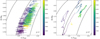	Fig. 5. Same as the right-hand panel of Fig. 4 but for p = 1 (left panel) and p = 2 (right panel).
In the text

	Fig. 6. Same as the right-hand panel of Fig. 4 but for D = 0.25 (left panel) and D = 1 (right panel).
In the text

	Fig. 7. Same as the right-hand panel of Fig. 4 but for a model with α = 10−7 and q given by Eq. (22). The horizontal red line corresponds to the Ωeq given by Eq. (24)
In the text

References

- Abolmasov, P., Nättilä, J., & Poutanen, J. 2020, A&A, 638, A142 [Google Scholar]
- Armitage, P. J. 2002, MNRAS, 330, 895 [Google Scholar]
- Belloni, T., Méndez, M., & Homan, J. 2005, A&A, 437, 209 [NASA ADS] [CrossRef] [EDP Sciences] [Google Scholar]
- Belyaev, M. A., Rafikov, R. R., & Stone, J. M. 2013, ApJ, 770, 67 [Google Scholar]
- Capano, C. D., Tews, I., Brown, S. M., et al. 2020, Nat. Astron., 4, 625 [Google Scholar]
- Gilfanov, M., & Arefiev, V. 2005, ArXiv e-prints [arXiv:astro-ph/0501215] [Google Scholar]
- Gilfanov, M., Revnivtsev, M., & Molkov, S. 2003, A&A, 410, 217 [NASA ADS] [CrossRef] [EDP Sciences] [Google Scholar]
- Hasinger, G., & van der Klis, M. 1989, A&A, 225, 79 [NASA ADS] [Google Scholar]
- Inogamov, N. A., & Sunyaev, R. A. 1999, Astron. Lett., 25, 269 [NASA ADS] [Google Scholar]
- Kluzniak, W., & Wagoner, R. V. 1985, ApJ, 297, 548 [Google Scholar]
- Landau, L. D., & Lifshitz, E. M. 1987, Fluid Mechanics (Pergamon: Cambridge) [Google Scholar]
- Lynden-Bell, D., & Pringle, J. E. 1974, MNRAS, 168, 603 [NASA ADS] [CrossRef] [Google Scholar]
- Méndez, M., & Belloni, T. 2007, MNRAS, 381, 790 [NASA ADS] [CrossRef] [Google Scholar]
- Méndez, M., van der Klis, M., Ford, E. C., Wijnands, R., & van Paradijs, J. 1999, ApJ, 511, L49 [NASA ADS] [CrossRef] [Google Scholar]
- Méndez, M., van der Klis, M., & Ford, E. C. 2001, ApJ, 561, 1016 [NASA ADS] [CrossRef] [Google Scholar]
- Miller, M. C. 2001, AIP Conf. Ser., 599, 229 [Google Scholar]
- Miller, M. C., Lamb, F. K., Dittmann, A. J., et al. 2019, ApJ, 887, L24 [Google Scholar]
- Nättilä, J., Miller, M. C., Steiner, A. W., et al. 2017, A&A, 608, A31 [NASA ADS] [CrossRef] [EDP Sciences] [Google Scholar]
- Nowak, M. A., Vaughan, B. A., Wilms, J., Dove, J. B., & Begelman, M. C. 1999, ApJ, 510, 874 [Google Scholar]
- Papaloizou, J. C. B., & Stanley, G. Q. G. 1986, MNRAS, 220, 593 [Google Scholar]
- Popham, R., & Narayan, R. 1995, ApJ, 442, 337 [Google Scholar]
- Revnivtsev, M. G., Suleimanov, V. F., & Poutanen, J. 2013, MNRAS, 434, 2355 [Google Scholar]
- Riley, T. E., Watts, A. L., Bogdanov, S., et al. 2019, ApJ, 887, L21 [NASA ADS] [CrossRef] [Google Scholar]
- Sibgatullin, N. R., & Sunyaev, R. A. 2000, Astron. Lett., 26, 699 [Google Scholar]
- Suleimanov, V., & Poutanen, J. 2006, MNRAS, 369, 2036 [Google Scholar]
- Uttley, P., McHardy, I. M., & Vaughan, S. 2005, MNRAS, 359, 345 [Google Scholar]
- van der Klis, M. 2000, ARA&A, 38, 717 [Google Scholar]
- van der Klis, M. 2001, ApJ, 561, 943 [Google Scholar]
- Vaughan, B. A., & Nowak, M. A. 1997, ApJ, 474, L43 [Google Scholar]