© ESO 2021

1 Introduction

Compared to reflectance spectroscopy, which is sensitive to mineralogy and chemical compositions, the phase curve of an airless body is more sensitive to regolith physical properties such as particle shape and transparency, size distribution, packing density, and macroscopic and microscopic surface roughness. The nonlinear increase of surface brightness in the anti-solar direction (the opposition effect (OE)), caused by shadow hiding and/or coherent back-scattering, is useful when inferring the regolith opaqueness, porosity, and particle size distribution (e.g., Helfenstein et al. 1997; Abe et al. 2006; Mishchenko 2008; Shkuratov et al. 2011; Hapke 2012). Various photometric models have been developed to describe light scattering properties of the surface regolith (e.g., Lumme & Bowell 1981; Muinonen 2004; Hapke et al. 2012; Mishchenko et al. 2015), and it has been recognized that a wide coverage of the solar phase angle is a crucial to reliably retrieving model parameters from the measurement.

Since the successful landing of the Chang’E-4 (CE-4) spacecraft in the Von Kármán crater (177.588°E, 45.4578°S) on the floor of the South Pole-Aitken basin (Fig. A.1) on Jan. 3, 2019 (Di et al. 2019a), the panorama cameras (PCAMs) onboard the Yutu-2 rover have extensively imaged the landing area. This has provided a good opportunity to study the regolith photometric properties in addition to its spectroscopic properties (e.g., Li et al. 2019; Hu et al. 2019). From this work, we extracted the in-situ lunar phase curves using the PCAM images and compared them with the Chang’E-3 (CE-3) measurement made in Mare Imbrium (Jin et al. 2015), which was the first of its kind since the Apollo era. By performing photometric model inversions using both the Hapke model (Hapke 2012) and the Lumme-Bowell model (Lumme & Bowell 1981, LB model hereafter), we infer the regolith physical properties and compare them with those of CE-3.

2 Instrument and data descriptions

As its backup payload, the Yutu-2 rover has a PCAM system identical to that of CE-3 (Jin et al. 2015). As shown in Fig. A.2, the left PCAM (PCAML) and right PCAM (PCAMR) are located on top of the mast and can rotate horizontally (0°–360° yaw) and vertically (−30° −0° pitch), withtheir horizontal pointing directions turned toward each other by 1°. The PCAMs can work in color and panchromatic modes with a field of view of 19.6° by 14.5° (Jia et al. 2018).

A more detailed description of the PCAM data product can be found in Ren et al. (2014). In brief, each level 2B (L2B) digital number (DN) image was obtained by applying a series of operations on level 0 raw data including format processing, dark current subtraction, and flat fielding correction. The gain, exposure time, and geometric information are also included in each 2B image as the header file. The geometric information includes the solar zenith and azimuth angles, the exterior orientation elements (T1), and the inner orientation elements (T2). Each L2B frame in color mode is 2352 by 1728 pixels and consists of four color bands with a Bayer filter mosaic arrangement: red (R, 640 nm), green (G1, 540 nm), green (G2, 540 nm), and blue (B, 470 nm). As the PCAM data with higher levels above L2B have undergone color interpretations and are released as color photos, they are not suitable for quantitative photometric analysis. Unfortunately, most PCAM data measured so far have been taken in panchromatic mode and thus we have selected the L2B data collected on the third lunar day for phase curve extractions.

Figure 1 shows a panoramic view of the study area, which is about 75 m west of the lander. This picture is a mosaic of 43 overlapping images taken by the PCAMR during the third lunar day, and the image IDs are listed in Table C.1. When selecting these images, we avoided pictures with the presence of obvious solar glares (Fig. A.3). A topographic analysis of the landing site (Di et al. 2019b) shows that the terrain is generally higher in the northeast than in the southwest, with an elevation drop of ~ 8 m over 350 m distance, corresponding to a slope angle of about 1°. Although there are decimeter-sized craters in the scene, the study area around the rover is otherwise flat, and therefore we can treat the surface as macroscopically flat with an identical solar zenith angle of 80° for all images in the mosaic. The actual solar zenith angle in various images ranges from 79.6635° to 80.2584°.

Fig. 1 Panoramic view of the study area imaged by the PCAMR with image IDs listed in Table C.1. The opposition effect is seen centred around the shadow of the PCAMR. The average solar zenith angle for these images is 80°.

Fig. 2 Example contour plots of the calculated viewing zenith angles (a) and phase angles (b) in phase curve extractions. Regions surrounded by dashed green lines are treated as shadows and are not used in phase curve extractions.

3 Phase-curve extraction

We followed the same procedure to extract the insitu lunar phase curves as we did for the CE-3 data (Jin et al. 2015) as summarized below:

First, we used T1 and T2 to calculate the vector (V1) from a pixel to the PCAMs through the collinearity equations and obtained the viewing zenith angle (e) for each pixel (Fig. 2a). Second, we used the solar zenith angle and solar azimuth angle in each image’s header file to calculate the vector (V2) from the pixel to the Sun. Then, the angle between V1 and V2, or the solar phase angle (α), can be obtained using vector algebra (Fig. 2b). Third, we removed pixels from the shadow of the rover (in the rover image) and pixels with e larger than 85° in all frames due to their lower collection efficiencies. The retrieved values are plotted as gray dots in Fig. 3, and those averaged within a 1° phase-angle bin are shown as the yellow dots. Fourth, we converted the L2B DN value of each pixel in the frame to radiance (I_s) with the brightness normalization parameter A_Cali and the absolute radiation calibration coefficients C_Rad provided by the payload team: $$I_{\text{s}}=\frac{DN}{A_{\text{Cali}}\cdot C_{\text{Rad}}},$$(1)

where A_Cali is recorded in each header file, and C_Rad (in Sr nm m²∕W) is 7.667 × 10⁵, 9.893 × 10⁵, 9.893 × 10⁵, and 9.705 × 10⁵ for the R, G1, G2, and B bands, respectively. Fifth, we averaged the radiance values of pixels within a 1° phase angle to reduce albedo variations caused by surface heterogeneities. Finally, we used the solar irradiance J(λ) (Gueymard 2004) to convert radiance to reflectance factor (REFF, r_s, Hapke 2012) as follows: $$r_{\text{s}}=\frac{\pi I_{\text{s}}}{\cos i{\displaystyle \int J}(\lambda )S(\lambda )\text{d}\lambda },$$(2)

where i is the solar zenith angle, and S(λ) is the normalized spectral response of the sensor provided by the payload team (the original response curves are shown in Fig. 4). All phase curves in this work are presented in terms of the REFF.

Figure 5 shows the comparisons of the CE-3 (Jin et al. 2015) and CE-4 phase curves in red, the CE-4 phase curves in R, G, and B, and the color ratios of CE-4. The gray dots in Fig. 5a are the original reflectance values, and the red curve with error bars is the averaged one within a 1° phase-angle bin for CE-4. Compared with that of the landing site of CE-3 in Mare Imbrium, the CE-4 phase curve has a lower absolute value (Fig. 5a) and a narrower opposition surge (Fig. 5b), implying the CE-4 site is more porous and/or the average CE-4 regolith is more transparent (e.g., Abe et al. 2006).

To remove the effects of different incident and view zenith angles between CE-3 and CE-4, in Figs. 5c–d we plot the reduced reflectance r_r (Hapke 2012) as $$r_{\text{r}}(i,e,\alpha )=\frac{I/F}{{\mu }_0/\left({\mu }_0+\mu \right)}=REFF\cdot \left({\mu }_0+\mu \right),$$(3)

where I∕F is the radiance factor, and μ₀ and μ are the cosine of i and e, respectively. Figure 5c shows that the reduced reflectance of CE-3 is about four-times higher than that of CE-4. After normalizing at 2° phase angle, the two curves still have marked differences (Fig. 5d), implying the different regolith physical properties of the two sites.

Many airless bodies have a steeper phase curve at shorter wavelength or have a redder reflectance spectrum at larger phase angles. This phase reddening effect has been observed for the Moon by Earth-based telescopes (e.g., Gehrels et al. 1964; McCord 1969), and orbiter (e.g., Hapke et al. 2012) and insitu measurements (Jin et al. 2015), and it has also been observed in laboratory experiments (e.g., Adams & Filice 1967; Johnson et al. 2013; Pommerol et al. 2013; Schröder et al. 2014). The color ratio spectra of CE-4 shown in Fig. 5f clearly show the phase reddening effect: the curves first drop from 1° to 3° and then increase sharply from 3° to about 40° and gradually approach a peak around 100° before decreasing again. The increase at phase angles larger than ~ 130° is similar to what happens in the CE-3 case (Jin et al. 2015) but is more pronounced. The phase curves in the G and B bands have error levels commensurate with the red one, which for clarity are not shown in Fig. 5e. The uncertainties of the color ratio curves (R/G and R/B), estimated from error propagation equations, are better than ~ 40%, which is the upper limit in case the covariances between the R, G, and B bands are zero.

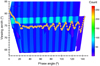Fig. 3 Extracted viewing zenith angles for all useful pixels (color dots represent pixel densities with a bin width of 0.15 in the phase angle axis and 0.021 in the viewing zenith axis) and the averaged values within a 1° phase-angle bin (yellow circles).

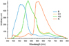Fig. 4 Spectral response functions of PCAM sensors provided by the payload team. B, G1, G2, and R represent the blue, green 1, green 2, and red pixels, respectively. The area of each of these functions was normalized to 1 when deriving the reflectance factor using Eq. (2).

4 Photometric model inversions

In order to compare the CE-3 and CE-4 landing-site photometric properties, we used the Hapke model (Hapke 2012) and the LB model (Lumme & Bowell 1981) to invert the reflectance phase curve. Although the physical significance of the model parameters has been a constant subject of debate (Mishchenko 1994; Hapke 1996, 2013; Hapke et al. 2009; Zhang & Voss 2011; Shkuratov et al. 2012), by comparing the fitting results of CE-3 and CE-4, useful conclusions in comparative planetology may be made. A comparison of similar parameters from different models may also help to verify the modeling results.

4.1 The Hapke model

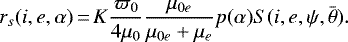
The Hapke model in reflectance factor (REFF) is given as (Hapke 2012; Hapke et al. 2012) $$\begin{array}{ll}\hfill & r_s(i,e,\alpha )=K\frac{{\varpi }_0}{4{\mu }_0}\frac{{\mu }_{0e}}{{\mu }_{0e}+{\mu }_e}\{[1+B_S(\alpha )]P(\alpha )\hfill \\ \hfill & +H({\mu }_{0e}/K)H({\mu }_e/K)-1\}[1+B_C(\alpha )]S(i,e,\psi ,\overline{\theta }),\hfill \end{array}$$(4)

where K is the porosity coefficient, ϖ₀ is the single-scattering albedo (SSALB), μ₀ is the cosine of theincident angle (i), and μ_0e and μ_e are cosines of the effective incident angle and the effective viewing zenith angle, respectively. To account for both backward- and forward-scattering lobes, a two-term Henyey-Greenstein phase function is used to approximate single-scattering phase function P(α) as $$\begin{array}{lll}P(\alpha )\hfill & =\hfill & \frac{1+c}{2}\frac{1-b^2}{{\left(1-2b\cos \alpha +b^2\right)}^{3/2}}+\frac{1-c}{2}\frac{1-b^2}{{\left(1+2b\cos \alpha +b^2\right)}^{3/2}},\hfill \\ \hfill & \hfill & \hfill \\ [-15pt]\hfill & \hfill & \hfill \end{array}$$(5)

with a corresponding asymmetry parameter ζ = −bc. The Ambartsumian-Chandrasekhar H function is approximated by 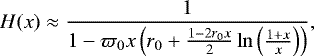$$H(x)\approx \frac{1}{1-{\varpi }_{0}x\left(r_0+\frac{1-2r_{0}x}{2}\ln \left(\frac{1+x}{x}\right)\right)},$$(6)

where r₀ is the diffusivereflectance given by $$r_0=\frac{1-\sqrt{1-{\varpi }_0}}{1+\sqrt{1-{\varpi }_0}}.$$(7)

The functions B_S(α) and B_C(α) describe the shadow-hiding opposition effect (SHOE) and the coherent-back-scattering opposition effect (CBOE) at small phase angle regionas $$B_S(\alpha )=\frac{B_{S0}}{1+\frac{1}{h_S}\tan \left(\frac{\alpha }{2}\right)},$$(8) $$B_C(\alpha )=B_{C0}\frac{1+[1-\exp (-\gamma )]/\gamma }{2{(1+\gamma )}^2},$$(9) $$\gamma =\frac{\tan (\alpha /2)}{h_C},$$(10)

and $S(i,e,\psi ,\overline{\theta })$ is the surface roughness factor with a mean slope angle $\overline{\theta }$ (Hapke 2012). For equant particles much larger than the radiation wavelength, K can be expressed as $$K=-\frac{\ln \left(1-1.209{\varphi }^{2/3}\right)}{1.209{\varphi }^{2/3}},$$(11)

where the ϕ (= 1-porosity) is the filling factor. For equant particles larger than the radiation wavelength and with a narrow particle size distribution, Eq. (9.26) from Hapke (2012) can be used to estimate the filling factor from h_S :

Fig. 5 Extracted phase curves and color ratio curves. (a) Comparisons of the CE-4 (orange, this work) and CE-3 (blue, Jin et al. 2015) phase curves in the R band (640 nm). For CE-4 data, the gray color dots represent pixel densities (with a bin width of 0.375 on the phase-angle axis and 0.000375 on the reflectance axis) of the original reflectance values and the red curve with error bars is the averaged value within a 1° phase angle; and (b) reflectance in the R band (640 nm) normalized at a 2° phase angle. We note that the minimum phase angle of the CE-4 phase curve is 1°, while that of CE-3 is 2°. (c) Reduced reflectance values obtained from Eq. (3); (d) reduced reflectance normalized at a 2° phase angle;(e) extracted phase curves in three colors for CE-4: red (R, 640 nm), green (G, the average of two 540 nm channels G1and G2), and blue (B, 470 nm); and (f) color ratios of red over blue and green over blue for CE-4.

$$h_S=\frac{3}{8}K\varphi .$$(12)

With the assumption that the regolith obeys a power-law size distribution (McKay et al. 1974), h_S can be used to estimate the particle size distribution as $$h_S=-0.537\frac{\ln \left(1-1.209{\varphi }^{2/3}\right)}{\ln \left(d_l/d_s\right)}{\varphi }^{1/3},$$(13)

where d_l and d_s are the diameters of the largest and smallest grains, respectively.

In brief, the Hapke fitting parameters used in this work are K, ϖ₀, b, c, B_S0, h_S, B_C0, h_C, and $\overline{\theta }$. The normal albedo (radiance factor at opposition) can be approximated by $$A_N\approx \frac{{\varpi }_0}{8}\left(1+B_{C0}\right)\left(1+B_{S0}\right)P(0).$$(14)

4.2 The LB model

The LB model (Lumme & Bowell 1981; Bowell et al. 1989) in REFF is expressed as: $$\begin{array}{ll}{r}_s(i,e,\alpha )=\hfill & \frac{2{\varpi }_{0}P(\alpha )}{4\left({\mu }_0+\mu \right)}{\Phi }_{\text{SH}}\frac{1+(1-\sigma )\rho \xi }{1+\rho \xi }\hfill \\ \hfill & +\frac{{\varpi }_0^{*}}{4\left({\mu }_0+\mu \right)}\left[H\left({\varpi }_0^{*},{\mu }_0\right)H\left({\varpi }_0^{*},\mu \right)-1\right],\hfill \end{array}$$(15)

where ϖ₀ and ${\varpi }_0^{*}$ are the original and the scaled SSALB, respectively: $${\varpi }_0^{*}=\frac{1-\zeta }{1-\zeta {\varpi }_0}{\varpi }_0.$$(16)

P(α) and H are given by Eqs. (5) and (6), respectively. σ is the fraction of surface area coveredby holes, and ρ is the surface roughness measured by the tangent of the mean surface slope angle, $\rho =\tan \overline{\theta }$. μ₀ and μ are cosines of the incident zenith i and viewing zenith e, respectively. The shadowing function Φ_SH can be approximated by (Peltoniemi & Lumme 1992): $${\Phi }_{\text{SH}}=\frac{y+\frac{3}{4}}{y+\frac{3}{2}}$$(17) $$y=\frac{\varphi }{2.38}\frac{{\mu }_0+\mu }{\sqrt{{\mu }_0^2+{\mu }^2-2{\mu }_0\mu \cos \alpha }},$$(18) $$\xi =\frac{\sqrt{{\mu }_0^2+{\mu }^2-2{\mu }_0\cdot \mu \cos \alpha }}{{\mu }_0\mu }$$

where ϕ is the filling factor. The LB model in this form has six free parameters: ϖ₀, b, c, ϕ, ρ, and σ.

4.3 Model fitting and results

Since curve fitting to multivariable models can be highly dependent on initial guess values, we used the following procedures to find the most likely fitting parameters.

For the Hapke model (Appendix B), we first fit the data in the phase-angle range of 20°–144°, where the opposition effects are negligible with regard to obtaining the initial guess values of K, ϖ₀, b, c, and $\overline{\theta }$. We find that the fit K value was consistently below 1, which is outside its valid domain (Hapke 2012), and therefore we set the constraint K ≥ 1 in all following steps. Next, we extended the fitting to the full range [1°–144°] to include the opposition surge [1°–20°] to estimate all nine parameters including B_S0, h_S, B_C0, and h_C. The resultant negative B_C0 value (−0.05) implies thatthe CBOE may have no contribution to the OE. Also, as is shown in Fig. B.5, multiple scattering contributes less than 14% to total reflectance at small phase angles. Thus we removed CBOE and the model parameter number was reduced to seven. Then a grid search took place with the initial guess values derived from the above procedures as ([lower, upper; step]; Appendix B) K = [1.0, 1.3;0.1], ϖ₀ = [0.05, 0.20;0.05], b = [0.3, 0.5;0.1], c = [−0.4, 0.3;0.1], $\overline{\theta }=[{26}^{°},{38}^{°};2^{°}]$, and B_S0 = [0.4, 0.9;0.1], h_S = [0.01, 0.15;0.02], with constraints K ≥ 1, 0 < b < 1, and − 1 < c < 1. The histograms of the seven resultant parameters are shown in Figs. 6a–g. The narrow histograms are likely caused by the constraint we set for K. Finally, the peak position values of the histograms were used as the initial guess values and the converged fitting results are as follows: K = 1.0 ± 2.9, ϖ₀ = 0.11 ± 0.28, b = 0.35 ± 0.04, c = −0.21 ± 0.06, $\overline{\theta }={30.0}^{°}\pm {4.5}^{°}$, B_S0 = 0.28 ± 0.16, h_S = 0.023 ± 0.013, and A_N = 0.026 ± 0.068, and the fit curve is shown in Fig. 6h. In comparison, the nine-parameter fitting results for the CE-3 data are as follows: $K={1.47}_{-0.07}^{+0.16}$, ${\varpi }_0={0.19}_{-0.3}^{+0.1}$, b = 0.30 ± 0.1, $c={0.08}_{-0.08}^{+0.12}$, $\overline{\theta }={17}^{°}{}_{-6^{°}}^{+1^{°}}$, $B_{S0}={0.52}_{-0.2}^{+0.3}$, $B_{C0}={0.47}_{-0.17}^{+0.15}$, h_S = 0.059 ± 0.01, h_C = 0.12 ± 0.01, and $A_N={0.15}_{-0.05}^{+0}$ (Jin et al. 2015).

For the LB model, we first applied a grid search with initial values of ϖ₀ = [0.15, 0.35;0.02], b = [0.1, 0.5;0.1], c = [−0.5, 0.5;0.1], ϕ = [0.1, 1;0.1], slope = [3°, 35°;3°], σ = [0.1, 1;0.1] for CE-3 and ϖ₀ = [0.01, 0.15;0.02], b = [0.1, 0.5;0.1], c = [−0.5, 0.5;0.1], ϕ = [0.1, 1;0.1], slope = [3°, 35°;3°], and σ = [0.1, 1;0.1] for CE-4. We also set the following constraints: 0 < ϖ₀ < 1, 0 < D < 1, 0 < σ < 1, according to their physical meanings. The histogram distributions of each resulting parameter are shown in Figs. 7a–f. The most probable values obtained areϖ₀ = 0.25; b = 0.31; c = 0.38; ϕ = 0.12; slope = 17.8°; σ = 0.99 for CE-3, and ϖ₀ = 0.040, b = 0.32, c = 0.40, ϕ = 0.0010, slope = 14.8°, σ = 0.99 for CE-4. These values were then used as initial guess values to fit the data, and the final fitting results are as follows: ϖ₀ = 0.22 ± 0.01, b = 0.32 ± 0.01, c = 0.58 ± 0.02, ϕ = 0.17 ± 0.11, ρ = 2.0 ± 1.9 (with a corresponding slope angle of ${63.4}^{°}{}_{-{57.7}^{°}}^{+{12.2}^{°}}$), σ = 0.34 ± 0.06 for CE-3 and ϖ₀ = 0.080 ± 0.017; b = 0.32 ± 0.04; c = 0.42 ± 0.27; ϕ = 0.0095 ± 0.0112; ρ = 0.32 ± 0.25 (with a corresponding slope angle of ${17.7}^{°}{}_{-{13.7}^{°}}^{+{12.0}^{°}}$), σ = 0.95 ± 0.36 for CE-4 as shown in Figs. 7h and 7i. The factor that caused the drop at small phase angles for CE-4 (Fig. 7i) is unknown. We noticed that this dip would disappear if the incident zenith angle were changed slightly (e.g., from 80° to 80.5°), but then it would appear at other slightly different values (e.g., 80.4°). Therefore, we did not attempt to make the fit look better by fine-tuning the incident angle, but we fixed the incident angle at 80°.

Fig. 6 Histograms of the fitted parameters of the seven-parameter Hapke model over the full phase angle range (1°–144°) with no CBOE contribution (BC(α) = 0) and with theconstraint K ≥ 1: (a) porosity factor K; (b) single scattering albedo ϖ0; (c) and (d) are b and c in Eq. (5); (e) slope angle $\overline{\theta }$; (f) and (g) are BS0 and hS in Eq. (8), respectively. The peak values of the (a)–(g) are then used as the initial guess values and the fitting results are shown in (h).

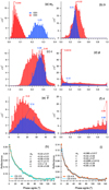Fig. 7 Fitting results of Lumme-Bowell model on CE-3’s and CE-4’s R-band data. Histograms of the grid searching results are shown in (a) to (f) as (a) ϖ0, (b) b, (c) c, (d) ϕ, (e) slope angle (°), and (f) σ. The fitting curves of (h) CE-3 and (i) CE-4 are also shown. ρ is the tangent of the slope angle, $\rho =\tan \overline{\theta }$.

5 Discussion

5.1 Phase reddening

The 3° minima in color ratios shown in Fig. 5f, not seen in the CE-3 data (Jin et al. 2015), appear to represent the colorimetric opposition effect (e.g., Shkuratov et al. 2011), which was found in laboratory measurements of lunar samples and remote sensing data (e.g., Akimov et al. 1979; Shkuratov et al. 1996; Hapke et al. 1998; Johnson et al. 2013; Kaydash et al. 2013). These minima still exist when we average the pixel values within a smaller phase angle bin, say 0.5°, and thus we believe it is not an artifact. The phase reddening effect is also quite certain as it occurs over a broad phase-angle range. The cause of the arched shape of the color ratio is believed to be related to the various contributions of volume scattering at various phase angles: in going from small to medium and then large phase angles, the mean optical path length increases and then decreases, so does the ratio of volume scattering to surface scattering (Adams & Filice 1967; Johnson et al. 2013). The overall pattern of the CE-4 color ratio is similar to that of CE-3 (Jin et al. 2015) but with a larger amplitude. This may be explained by the fact that the CE-4 landing site has redder reflectance spectra than CE-3 and according to the laboratory study by Schröder et al. (2014), redder reflectance spectra have a stronger phase reddening effect. The fact that the maximum of the arch appears at very large phase angles may be caused by the large incident angle of 80° (Schröder et al. 2014) for the CE-4 data here.

5.2 Model parameter interpretations

The final fitting results of the CE-3 and CE-4 data phase curves using the two models are summarized in Table 1. It should be noted that the porosity coefficient K retrieved by the Hapke model for CE-4 is 1.0, leading to a filling factor of 0 according to Eq. (11). Therefore, Eq. (12) was used to estimate ϕ for CE-4. Table 1 shows that three out of the four parameters that both models contain, ϖ₀, ϕ, and ζ, have similar differential behaviors despite their different absolute values: although the LB ϖ₀ differ from the Hapke ϖ₀ by 20− 30%, both are lower for CE-4 than CE-3 by about 50%, which is consistent with the much lower values of both spectral reflectance (Hu et al. 2019) and phase curves (this work) of the CE-4 landing site. On one hand, we notice that many photometric modelings using the Hapke model retrieved similar low SSALB values (e.g., Beck et al. 2012; Sato et al. 2014). On the other hand, we recognize that these SSALB values may be too low to be considered realistic, as Mie calculations can hardly produce SSALB lower than 0.6 or so, even for highly absorbing grains. Therefore, the retrieved SSALB values should be interpreted more in a comparative sense. The filling factors ϕ retrieved by both models are consistently much lower for the CE-4 site (~ 6% by Hapke and ~ 1% by LB) than for the CE-3 (~32% by Hapke and ~17% by LB), indicating that the regolith of the former is more porous than that of the latter. Due to the long-term space weathering processes and the Moon’s low gravity, the porosity of the uppermost regolith layer is believed to be very high. Hapke & Sato (2016) confirmed the high porosity values (74–87%) of the uppermost layer of lunar regolith derived by Ohtake et al. (2010) and concluded this may be a lower limit. Although our retrieval results (porosity >90%) are basically commensurate with these values, as the rover did not photograph any (nearly) levitating particles on the surface, our retrieved porosity values should be more of comparative significance. The asymmetry parameters ζ retrieved by the two models have opposite signs for both the CE-3 and CE-4 landing sites; however, both are more positive for CE-4 than CE-3, indicating the CE-4 regolith is more forward scattering. With a fit h_S ~ 0.023, the ratio of the largest and smallest particle diameters d_l∕d_s can be estimated by Eq. (13) as ~7, in contrast to ~46 for CE-3, suggesting a much narrower size distribution at the CE-4 site than the CE-3 (The d_l ∕d_s estimated from Eq. (11) for CE-3 is ~180). Even the absolute accuracy of these model parameters cannot be evaluated or justified, the semi-quantitative and qualitative agreement between twomodel parameters can give us confidence in comparing the model parameters between the CE-3 and CE-4 landing sites. The lower B_S0 value by theHapke model, 0.28 for CE-4 and 0.52 for CE-3, indicates the CE-4 regolith is more transparent and this larger transparency may have caused the regolith layer to be more forward scattering.

The conclusion that coherent back-scattering (CBS) is absent at CE-4’s landing site comes mainly from the fact that the Hapke model fitting did not return physically possible CBS parameters. Considering the fact that CE-4’s landing site is very dark and the solar zenith angles when taking the PCAM images were very large (~ 80°), it is possible that multiple scattering is weak, and thus the CBS contribution is small. However, recent numerical simulations (e.g., Muinonen et al. 2012, 2018; Markkanen et al. 2018) and laboratory measurements (Hapke et al. 1993; Nelson et al. 1998, 2000) show that CBS could be present on dark surfaces. Therefore, the possible presence of the CBS in CE-4 phase curves cannot be completely ruled out, and its exclusion may have led to the very high porosity value derived from the Hapke model.

As the landing site surface ages of CE-3 and CE-4 have been estimated to be ~ 3 Ga and ~3.6 Ga, respectively (e.g., Hiesinger et al. 2000; Fa et al. 2015; Pasckert et al. 2018), the surface material of the latter may have experienced a higher level of space weathering including meteorite bombardment and comminution, and thus have become darker and finer with a narrower size distribution. The much lower normal albedo value at the CE-4 site (~ 0.03) compared tothat of CE-3 (0.15), together with the fact that the CE-4 site shows no signs of albedo increase caused by descent engine blow¹, also supportthis argument. The higher transparency of the CE-4 regolith could be caused by the higher concentrations of glassy materials generated by space weathering, but this speculation would need further investigation, as other factors such as different mineralogies(Zhang et al. 2015; Hu et al. 2019) may also play a role.

For slope angle $\overline{\theta }$, the two models did not return consistent values between the CE-3 and CE-4 sites. Although neither model specified the valid spatial scales of its model roughness, the scales of the “macroscopic roughness” (Hapke 2012) and “depth-to-radius ratio of a hole” (Lumme & Bowell 1981) are both likely below ~ 8 cm (Helfenstein & Shepard 1999). In comparison, Rozitis & Green (2011) derived the root mean square (RMS) slope of the Moon’s entire surface to be ~ 32° at scales from thermal skin depth (~1 cm) to observational spatial resolution (~18 km). A topographical study using Kaguya’s Terrain Camera dataset with a 30 m baseline found the CE-4 landing area is flat, with 90% of the surface having slopes of less than 5° (Qiao et al. 2019). By studying the Apollo Lunar Surface Closeup Camera pictures, Helfenstein & Shepard (1999) found the RMS slope at a 1 mm scale is ~ 16° for the lunar mare and ~25° for the highland. The Hapke $\overline{\theta }$ values (~17° for CE-3 and ~30° for CE-4) are close to that of Helfenstein & Shepard (1999) and these are consistent with the fact that the lunar highlands are photometrically rougher than the mares. Since the spatial scale that $\overline{\theta }$ characterizes may also depend on surface albedo (Helfenstein & Shepard 1999), and the CE-3 regolith is much brighter with stronger multiple scattering, it is possible that CE-3’s $\overline{\theta }$ has a larger spatial scale than that of CE-4. The LB $\overline{\theta }$ (~ 63°) for CE-3 is probably too large, as in Fig. 7e most $\overline{\theta }$ values are concentrated below 20°. In short, the Hapke $\overline{\theta }$ values for CE-3 and CE-4 may be realistic on millimeter and centimeter scales and are not inconsistent with the result from Qiao et al. (2019) as they were made at different spatial scales.

5.3 Comparison with remote sensing measurement

To compare with remote sensing measurements of lunar highland at 643 nm made by Sato et al. (2014), we also fit the Hapke model to the CE-4 data with fewer parameters. Since the maximum phase angle of Sato et al. (2014) is 97°, we carried out fittings over the full phase angle range (1–144°) and over (1–97°) as well (Appendix B.2, Figs. B.7–B.10, Table 2). The principal results are as follows: (1) our ϖ₀, 0.082, is smaller than their value, 0.42, which is consistent with the darker nature of the CE-4 landing site; (2) our b (0.34) and c (−0.085) are close to the typical highland crystalline in the “hockey-stick” graph (Fig. 8); (3) our h_S, 0.037, is smaller than their 0.080, indicating we are seeing a narrower size distribution (this does not contradict the above CE-3/CE-4 comparison, however); (4) our B_S0, 0.52, is smaller than their value of 1.7, suggesting that we observe more transparent grains.

Sato et al. (2014) found that, in general, the lunar surface with higher level of maturity is more forward scattering, though mineralogy must be considered when making comparisons (e.g., the anorthosite-rich but ilmenite-poor highland material and the ilmenite-rich mare material may have different scattering properties). On the other hand, in our laboratory photometric study of analog materials including lunar regolith simulant, silicates, and ilmenite before and after simulated space weathering, we found that the back-scattering lobes of five out of the six samples became stronger with more negative asymmetry parameters of the single-scattering phase functions after laser irradiations (Jiang et al. 2019). Reflectance spectroscopy shows that the CE-4 regolith is redder with more subdued absorption features than the CE-3 regolith (Zhang et al. 2015; Hu et al. 2019), indicating the former is more mature and therefore, should be more back scattering. In this study, both photometric models have returned more positive asymmetry parameters for the CE-4 site than CE-3 (Table 1). Thus, according to the result of Sato et al. (2014), the CE-4 site should be more mature than that of CE-3, consistently with the spectroscopic results. The contradiction with our laboratory measurement is expected to be solved by performing more laboratory and modeling work in the future.

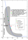Fig. 8 Typical values of b and c (Henyey-Greenstein phase-function parameters) for the mature mare (low and high Ti content), the mature highland, and the immature highland ejecta in 643 nm band parameter maps by Sato et al. (2014). The red horizontal double triangle indicates the b and c values derived in B.2. The blue vertical double triangle represents the b and c values of CE-3 in Jin et al. (2015).

6 Summary and conclusion

We extracted the phase curves of CE-4’s landing site using the panorama camera images measured by the Yutu-2 rover and carried out photometric inversions using the Hapke model and the Lumme-Bowell model. We obtained the following results: compared with the insitu lunar phase curves measured by CE -3, the CE -4 phase curves have lower reflectance values and are relatively steeper, have a stronger phase-reddening effect, and show the colorimetric opposition effect. The Hapke model and the Lumme-Bowell model returned qualitatively consistent results in a single-scattering albedo, porosity, and an asymmetry parameter, which shows that the CE-4 regolith is much darker, more porous, and more forward scattering than that of CE-3. The Hapke model shows the CE-4 site is rougher than the CE-3 site. These features indicate that the surface materials at the CE-4 landing site are more mature than those of CE-3.

Even concerning parameters for which the two models yielded consistent results, their absolute values are not guaranteed to be physically correct. Therefore, more focus should be placed on their interpretations in comparative analysis.

Acknowledgements

We thank Karri Muinonen for critical comments that improved the quality of the manuscript. We thank the Chang’E payload team for mission operations and China National Space Administration for providing the Chang’E data that made this study possible. This work was supported by the National Natural Science Foundation of China (11773023, 11941001, U1631124, 11941002) and the Civil Aerospace Pre-research Project (D020302). M.-H.Z. was supported by the Science and Technology Development Fund, Macau (0079/2018/A2) and the pre-research project on Civil Aerospace Technologies No. D020202 funded by China National Space Administration (CNSA). The Chang’E data used in this work were processed and produced by the Ground Research and Application System of China’s Lunar Exploration Program and can be downloaded at http://moon.bao.ac.cn/searchOrder_dataSearchData.search.

Appendix A More information on the landing site and images

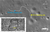Fig. A.1 Location of CE-4 landing site and PCAM measurement site. The white line indicates the Yutu-2 Rover’s path during the first three lunar days. The base image was photographed by the landing camera onboard the CE-4 spacecraft. The inset shows the Lunar Reconnaissance Orbiter Camera Wide Angle Camera mosaic of the surrounding region of the CE-4 landing site in the South Pole-Aitken basin.

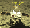Fig. A.2 Arrangement of PCAMs on CE-4’s rover Yutu-2. PCAML and PCAMR are indicated by yellow arrows.

Fig. A.3 All images taken by PCAMR in color mode during the third lunar day. Obviously, images with numbers in yellow are identified as glare-contaminated, and thus are not used in mosaicing.

Appendix B Detailed procedures for fitting the Hapke model

B.1 A piecewise fitting approach

To avoid any possible initial guess value-dependent fitting uncertainties, we performed a grid search in parameter space to obtain a more reliable fitting result. The fitting steps are summarized in Fig. B.1 and are described as follows.

Fig. B.1 Flowchart of Hapke model fitting process.

B.1.1 Step 1: fitting of the phase curve in a phase-angle range with no opposition surge (20°–144°) using the five-parameter model

We first fit the phase curve in the phase angle range with no opposition surge (20°–144°) by setting B_S(α) and B_C(α) in Eq. (4) to zero to obtain the initial guess values of the rest five parameters: K, ϖ₀, b, c, and $\overline{\theta }$. By varying these five parameters from lower to upper bounds with steps ([lower, upper; step]) as: K = [0.3, 1.8; 0.2], ϖ₀ = [0.05, 0.5; 0.1], b = [0, 0.5; 0.1], c = [-0.5, 0.5; 0.3], and $\overline{\theta }$ = [10°, 35°; 3°], we obtained the histograms (Figs. B.2a–e) of the distributions of these five parameters. By using the peak values in these five histograms as the initial guess values, we obtain the fitting result shown in Fig. B.2f. It can be seen that the fitted K value 0.074 is unphysical as by definition (Eq. (11)) it should be larger than or equal to 1. Figure B.2a also shows that the porosity factor K has large amount of values concentrated in regions of smaller than 1. To make the fitting results more physically plausible, we repeated the above step with K constrained to be larger or equal to 1, and the results are shown in Fig. B.2. The peak values of the histograms in Figs. B.3a–e, K = 1.0, ϖ₀ = 0.11, b = 0.35, c = −0.23, $\overline{\theta }$ = 32.5°, were then used as the initial fitting parameters, and the resultant fitting is shown in Fig. B.3f. Although now the fit K has a larger spread, the central value 1.0 does not contradict its definition.

B.1.2 Step 2: fitting the phase curve using the nine-parameter Hapke model over the full phase-angle range (1°–144°)

In this step, we performed the fitting using the full model including the shadow-hiding (B_S0, h_S) and coherent-back-scattering (B_C0, h_C) contributions over the full phase-angle range (1°–144°). Based on the results shown in Figs. B.3a–f, we chose the grid values as follows: [lower, upper; step] as: K = [1, 1.3; 0.1], ϖ₀ = [0.05, 0.2; 0.05], b = [0.1, 0.5; 0.1], c = [−0.5, 0.1; 0.2], $\overline{\theta }$ = [25°, 40°; 5°], B_S0 = [0.4, 1; 0.2], h_S = [0.05, 0.15; 0.05], B_C0 = [0.4, 1; 0.2], and h_C = [0.05, 0.2; 0.05]. With these 245,760 combinations as initial guess values, nonlinear least square fittings of Eq. (4) were performed, and the resultant parameter histograms are shown in Figs. B.4a–i. With these peak values as the initial fitting guessvalues, the nine-parameter fitting was performed again, and the fitting result is shown in Fig. B.4j.

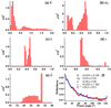Fig. B.2 Histograms of fit parameters ((a) porosity factor K; (b) single-scattering albedo ϖ0; (c) and (d) are b and c in Eq. (5); and (e) slope angle $\overline{\theta }$) of theHapke model with no SHOE and CBS terms over the phase-angle range (20°–144°). The final fitting result (f) was obtained using the peak values retrieved from (a) to (e) as initial guess values.

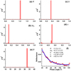Fig. B.3 Histograms of fit model parameters ((a) porosity factor K; (b) single-scattering albedo ϖ0; (c) and (d) are b and c in Eq. (5); (e) slope angle $\overline{\theta }$) of the five-parameter Hapke model fitting with no opposition terms (by setting BS (α) = 0 and BC (α) = 0 in Eq. (4) over the phase angle range (20°–144°) with K constrained to be larger than or equal to 1. The peak values of the parameters in (a)–(e) were then used as the initial guess values in the fitting and the final results are shown in (f).

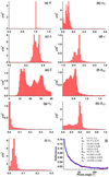Fig. B.4 Histograms of fit parameters ((a) porosity factor K; (b) single-scattering albedo ϖ0; (c) and (d) are b and c in Eq. (5); (e) slope angle $\overline{\theta }$; (f) and (g) are BS0 and hS in Eq. (8); and (h) and (i) are BC0 and hC in Eq. (9)) of the nine-parameter Hapke model over the full phas- angle range (1°–144°) with K constrained to be larger than or equal to 1. The peak values of (a)–(i) were then used as the initial guess values, and the fitting results are shown in (j).

B.1.3 Step 3: seven-parameter fitting for the full phase angle range (1°–144°)

Since the fit B_C0 value from Step 2 is −0.050 (Fig. B.4j), the coherent-back-scattering (CBOE) contribution may be negligible. To observe this, in Fig. B.5 we plot the estimated multiple-scattering contribution by using Eq. (B.1) to approximate the single-scattering contribution with the parameters obtained in Step 2 (shown in Fig. B.4j): $$r_s(i,e,\alpha )=K\frac{{\varpi }_0}{4{\mu }_0}\frac{{\mu }_{0e}}{{\mu }_{0e}+{\mu }_e}p(\alpha )S(i,e,\psi ,\overline{\theta }).$$(B.1)

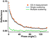Fig. B.5 Estimated contributions of multiple scattering (green curve) and single scattering (blue) to the CE-4 measured phase curve (red dots) by approximating a single scattering by Eq. (B.1). The single-scattering parameters used (K = 1.0, ϖ0 = 0.11, b = 0.35, c = −0.22, $\overline{\theta }$ = 30.4°) were obtained from Step 2, Fig. B.4j. The multiple scattering is calculated by subtracting single scattering from the CE-4 measurement.

Obviously, Fig. B.5 indicates that multiple scattering plays a minor role in the CE-4 phase curve, and as a result we can safely ignore the CBS contribution. By removing the CBOE terms in Eq. (4), the nine-parameter model has now been reduced to a seven-parameter version. By supplying the initial guess values ([lower, upper; step]) as follows: K = [1, 1.3; 0.1], ϖ₀ = [0.05, 0.2; 0.05], b = [0.3, 0.5; 0.1], c = [−0.4, 0.3; 0.1], $\overline{\theta }$ = [26°, 38°; 2°], B_S0 = [0.4, 0.9; 0.1], and h_S = [0.01, 0.15; 0.02], the fit parameter histograms are shown in Figs. B.6a–g. The peak values in Figs. B.6a–g were then used as the initial guess values, and the final fitting results of the seven-parameter model are obtained as K = 1.0 ± 2.9, ϖ₀ = 0.11 ± 0.28, b = 0.35 ± 0.04, c = −0.21 ± 0.06, $\overline{\theta }$ = 30.0° ± 4.5°, B_S0 = 0.28 ± 0.16, and h_S = 0.023 ± 0.013. During this final fitting step, the parameters ϖ₀, b, c, $\overline{\theta }$ are quite stable and appear plausible. With K constrained to be larger than or equal to 1, the fit K always stays near 1. Since the fit B_S0 value is below 1, the shadow-hiding term alone should be sufficient to describe the opposition effect. The very narrow histograms were probably a consequence of constraining K in the seven-parameter model fitting. The fitting results obtained in each of the above procedures are summarized in Table B.1.

B.2 Comparisons with Sato’s Hapke fitting to lunar global data

Sato et al. (2014) mapped the Hapke parameters over the Moon using a simplified version with three parameters (ϖ₀, b, B_S0, and h_S, but with ϖ₀ and B_S0 correlated through Eq. (B.3) below). They correlated b with c through Eq. (B.2) and B_S0 with ϖ₀ through Eq. (B.3) and fixed the slope angle to $\overline{\theta }$ = 23.4°. These simplifications allowed quicker computations of large amounts of data: $$c=3.29e^{-17.4b^2}-0.908,$$(B.2) $$B_{S0}\approx \frac{S(0)}{{\varpi }_{0}p(0)},$$(B.3)

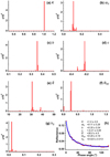Fig. B.6 Histograms of fit parameters ((a) porosity factor K; (b) single-scattering albedo ϖ0; (c) and (d) are b and c in Eq. (5); (e) slope angle $\overline{\theta }$; and (f) and (g) are BS0 and hS in Eq. (8)) of the seven-parameter Hapke model over the full phase-angle range (1°–144°) with no CBOE contribution (BC(α) = 0) and with K constrained to be larger than or equal to 1. The peak values of (a)–(g) are then used as the initial guess values and the fitting results are shown in (h).

where S(0) is the light scattered into the zero phase angle from the illuminated part of the particle surface, and ϖ₀ p(0) is the total light scattered from the particle into zero phase angle.

To compare our CE-4 data with those of Sato et al. (2014), we first used the same three-parameter model with a fixed slope angle (23.4°) but found this model to be incapable of fitting the measurement well (Fig. B.7d). Thus, we relaxed the correlations of Eqs. (B.2) and (B.3) and used the model with five free parameters (ϖ₀, b, c, B_S0, and h_S) with a fixed $\overline{\theta }$ = 23.4°. Again, we used the grid search method to find the most probable fitting parameters (Figs. B.8a-e): ϖ₀ = 0.090, b = 0.35, c = −0.090, B_S0 = 0.50, and h_S = 0.040 (also summarized in Table 2), and we used these as the initial guess values to obtain the final fitting result shown in Fig. B.8f.

It should be noted that the maximum phase angle in the data of Sato et al. (2014) is 97°, while ours is 144°. To understand if such a difference in phase angle coverage would affect the fitting results, we also fit the above three-parameter and five-parameter models within a 97° phase angle, and the results are shown in Figs. B.9 and B.10 and summarized in Table 2.

Obviously, the three-parameter model fitting over 1°–97° is still less satisfactory (Fig. B.9d), and the five-parameter fitting over 1°–97° (Fig. B.10f) produced very a similar result to that over 1°–144° (Fig. B.8f), with the largest difference being in the c parameter. To be consistent with our CE-4 data, we chose the b and c values derived from the five-parameter model over 1–144° to compare with the results of Sato et al. (2014). The b and c parameters for both CE-3 and CE-4 are added to the “hockey-stick” plot (McGuire & Hapke 1995) in Fig. 8.

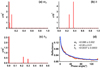Fig. B.7 Histograms of fit parameters ((a) single-scattering albedo ϖ0; (b) b; and (c) hS) of the simplified Hapke model over the full phase-angle range (1°–144°). The peak values of (a)–(c) were then used as the initial guess values, and the fitting results are shown in (d).

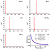Fig. B.8 Histograms of fit parameters ((a) single-scattering albedo ϖ0; (b) and (c) are b and c in Eq. (5); and (d) and (e) are BS0 and hS in Eq. (8)) of the five-parameter Hapke model over the full phase-angle range (1°–144°). The peak values of (a)–(e) are then used as the initial guess values, and the fitting results are shown in (f).

Fig. B.9 Same as in Fig. B.7 but over the phase-angle range (1°–97°).

Fig. B.10 Same as in Fig. B.8 but over the phase-angle range (1°–97°).

Appendix C List of all data file names used in this work

References

All Tables

All Figures

	Fig. 1 Panoramic view of the study area imaged by the PCAMR with image IDs listed in Table C.1. The opposition effect is seen centred around the shadow of the PCAMR. The average solar zenith angle for these images is 80°.
In the text

	Fig. 2 Example contour plots of the calculated viewing zenith angles (a) and phase angles (b) in phase curve extractions. Regions surrounded by dashed green lines are treated as shadows and are not used in phase curve extractions.
In the text

	Fig. 3 Extracted viewing zenith angles for all useful pixels (color dots represent pixel densities with a bin width of 0.15 in the phase angle axis and 0.021 in the viewing zenith axis) and the averaged values within a 1° phase-angle bin (yellow circles).
In the text

	Fig. 4 Spectral response functions of PCAM sensors provided by the payload team. B, G1, G2, and R represent the blue, green 1, green 2, and red pixels, respectively. The area of each of these functions was normalized to 1 when deriving the reflectance factor using Eq. (2).
In the text

Fig. 5 Extracted phase curves and color ratio curves. (a) Comparisons of the CE-4 (orange, this work) and CE-3 (blue, Jin et al. 2015) phase curves in the R band (640 nm). For CE-4 data, the gray color dots represent pixel densities (with a bin width of 0.375 on the phase-angle axis and 0.000375 on the reflectance axis) of the original reflectance values and the red curve with error bars is the averaged value within a 1° phase angle; and (b) reflectance in the R band (640 nm) normalized at a 2° phase angle. We note that the minimum phase angle of the CE-4 phase curve is 1°, while that of CE-3 is 2°. (c) Reduced reflectance values obtained from Eq. (3); (d) reduced reflectance normalized at a 2° phase angle;(e) extracted phase curves in three colors for CE-4: red (R, 640 nm), green (G, the average of two 540 nm channels G1and G2), and blue (B, 470 nm); and (f) color ratios of red over blue and green over blue for CE-4.

In the text

Fig. 6 Histograms of the fitted parameters of the seven-parameter Hapke model over the full phase angle range (1°–144°) with no CBOE contribution (BC(α) = 0) and with theconstraint K ≥ 1: (a) porosity factor K; (b) single scattering albedo ϖ0; (c) and (d) are b and c in Eq. (5); (e) slope angle $\overline{\theta }$; (f) and (g) are BS0 and hS in Eq. (8), respectively. The peak values of the (a)–(g) are then used as the initial guess values and the fitting results are shown in (h).

In the text

	Fig. 7 Fitting results of Lumme-Bowell model on CE-3’s and CE-4’s R-band data. Histograms of the grid searching results are shown in (a) to (f) as (a) ϖ0, (b) b, (c) c, (d) ϕ, (e) slope angle (°), and (f) σ. The fitting curves of (h) CE-3 and (i) CE-4 are also shown. ρ is the tangent of the slope angle, $\rho =\tan \overline{\theta }$.
In the text

Fig. 8 Typical values of b and c (Henyey-Greenstein phase-function parameters) for the mature mare (low and high Ti content), the mature highland, and the immature highland ejecta in 643 nm band parameter maps by Sato et al. (2014). The red horizontal double triangle indicates the b and c values derived in B.2. The blue vertical double triangle represents the b and c values of CE-3 in Jin et al. (2015).

In the text

	Fig. A.1 Location of CE-4 landing site and PCAM measurement site. The white line indicates the Yutu-2 Rover’s path during the first three lunar days. The base image was photographed by the landing camera onboard the CE-4 spacecraft. The inset shows the Lunar Reconnaissance Orbiter Camera Wide Angle Camera mosaic of the surrounding region of the CE-4 landing site in the South Pole-Aitken basin.
In the text

	Fig. A.2 Arrangement of PCAMs on CE-4’s rover Yutu-2. PCAML and PCAMR are indicated by yellow arrows.
In the text

	Fig. A.3 All images taken by PCAMR in color mode during the third lunar day. Obviously, images with numbers in yellow are identified as glare-contaminated, and thus are not used in mosaicing.
In the text

	Fig. B.1 Flowchart of Hapke model fitting process.
In the text

	Fig. B.2 Histograms of fit parameters ((a) porosity factor K; (b) single-scattering albedo ϖ0; (c) and (d) are b and c in Eq. (5); and (e) slope angle $\overline{\theta }$) of theHapke model with no SHOE and CBS terms over the phase-angle range (20°–144°). The final fitting result (f) was obtained using the peak values retrieved from (a) to (e) as initial guess values.
In the text

Fig. B.3 Histograms of fit model parameters ((a) porosity factor K; (b) single-scattering albedo ϖ0; (c) and (d) are b and c in Eq. (5); (e) slope angle $\overline{\theta }$) of the five-parameter Hapke model fitting with no opposition terms (by setting BS (α) = 0 and BC (α) = 0 in Eq. (4) over the phase angle range (20°–144°) with K constrained to be larger than or equal to 1. The peak values of the parameters in (a)–(e) were then used as the initial guess values in the fitting and the final results are shown in (f).

In the text

Fig. B.4 Histograms of fit parameters ((a) porosity factor K; (b) single-scattering albedo ϖ0; (c) and (d) are b and c in Eq. (5); (e) slope angle $\overline{\theta }$; (f) and (g) are BS0 and hS in Eq. (8); and (h) and (i) are BC0 and hC in Eq. (9)) of the nine-parameter Hapke model over the full phas- angle range (1°–144°) with K constrained to be larger than or equal to 1. The peak values of (a)–(i) were then used as the initial guess values, and the fitting results are shown in (j).

In the text

Fig. B.5 Estimated contributions of multiple scattering (green curve) and single scattering (blue) to the CE-4 measured phase curve (red dots) by approximating a single scattering by Eq. (B.1). The single-scattering parameters used (K = 1.0, ϖ0 = 0.11, b = 0.35, c = −0.22, $\overline{\theta }$ = 30.4°) were obtained from Step 2, Fig. B.4j. The multiple scattering is calculated by subtracting single scattering from the CE-4 measurement.

In the text

Fig. B.6 Histograms of fit parameters ((a) porosity factor K; (b) single-scattering albedo ϖ0; (c) and (d) are b and c in Eq. (5); (e) slope angle $\overline{\theta }$; and (f) and (g) are BS0 and hS in Eq. (8)) of the seven-parameter Hapke model over the full phase-angle range (1°–144°) with no CBOE contribution (BC(α) = 0) and with K constrained to be larger than or equal to 1. The peak values of (a)–(g) are then used as the initial guess values and the fitting results are shown in (h).

In the text

	Fig. B.7 Histograms of fit parameters ((a) single-scattering albedo ϖ0; (b) b; and (c) hS) of the simplified Hapke model over the full phase-angle range (1°–144°). The peak values of (a)–(c) were then used as the initial guess values, and the fitting results are shown in (d).
In the text

	Fig. B.8 Histograms of fit parameters ((a) single-scattering albedo ϖ0; (b) and (c) are b and c in Eq. (5); and (d) and (e) are BS0 and hS in Eq. (8)) of the five-parameter Hapke model over the full phase-angle range (1°–144°). The peak values of (a)–(e) are then used as the initial guess values, and the fitting results are shown in (f).
In the text

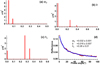	Fig. B.9 Same as in Fig. B.7 but over the phase-angle range (1°–97°).
In the text

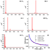	Fig. B.10 Same as in Fig. B.8 but over the phase-angle range (1°–97°).
In the text

References

- Abe, M., Takagi, Y., Kitazato, K., et al. 2006, Science, 312, 1334 [NASA ADS] [CrossRef] [Google Scholar]
- Adams, J. B., & Filice, A. L. 1967, J. Geophys. Res., 72, 5705 [CrossRef] [Google Scholar]
- Akimov, L. A., Antipova-Karataeva, I. I., & Shkuratov, T. G. 1979, in Lunar and Planetary Science Conference, 9 [Google Scholar]
- Beck, P., Pommerol, A., Thomas, N., et al. 2012, Icarus, 218, 364 [NASA ADS] [CrossRef] [Google Scholar]
- Bowell, E., Hapke, B., Domingue, D., et al. 1989, in Asteroids II, eds. R. P. Binzel, T. Gehrels, & M. S. Matthews (Tucson: University of Arizona Press), 524 [Google Scholar]
- Di, K., Liu, Z., Liu, B., et al. 2019a, J. Rem. Sensing, 23, 177 [Google Scholar]
- Di, K., Zhu, M.-H., Yue, Z., et al. 2019b, Geophys. Res. Lett., 46, 12, 764 [NASA ADS] [CrossRef] [Google Scholar]
- Fa, W., Zhu, M. H., & Liu, T. 2015, in European Planetary Science Congress, EPSC2015–190 [Google Scholar]
- Gehrels, T., Coffeen, T., & Owings, D. 1964, AJ, 69, 826 [NASA ADS] [CrossRef] [Google Scholar]
- Gueymard, C. A. 2004, Sol. Energy, 76, 423 [NASA ADS] [CrossRef] [Google Scholar]
- Hapke, B. 1996, J. Quant. Spectr. Rad. Transf., 55, 837 [CrossRef] [Google Scholar]
- Hapke, B. 2012, Theory of reflectance and emittance spectroscopy (Cambridge: Cambridge university press) [Google Scholar]
- Hapke, B. 2013, J. Quant. Spectr. Rad. Transf., 116, 184 [NASA ADS] [CrossRef] [Google Scholar]
- Hapke, B., & Sato, H. 2016, Icarus, 273, 75 [NASA ADS] [CrossRef] [Google Scholar]
- Hapke, B. W., Nelson, R. M., & Smythe, W. D. 1993, Science, 260, 509 [NASA ADS] [CrossRef] [PubMed] [Google Scholar]
- Hapke, B., Nelson, R., & Smythe, W. 1998, Icarus, 133, 89 [NASA ADS] [CrossRef] [Google Scholar]
- Hapke, B. W., Shepard, M. K., Nelson, R. M., Smythe, W. D., & Piatek, J. L. 2009, Icarus, 199, 210 [CrossRef] [Google Scholar]
- Hapke, B., Denevi, B., Sato, H., Braden, S., & Robinson, M. 2012, J. Geophys. Res. Planets, 117, E00H15 [CrossRef] [Google Scholar]
- Helfenstein, P., & Shepard, M. K. 1999, Icarus, 141, 107 [CrossRef] [Google Scholar]
- Helfenstein, P., Veverka, J., & Hillier, J. 1997, Icarus, 128, 2 [NASA ADS] [CrossRef] [Google Scholar]
- Hiesinger, H., Jaumann, R., Neukam, G., & Head, J. W. 2000, J. Geophys. Res., 105, 29239 [CrossRef] [Google Scholar]
- Hu, X., Ma, P., Yang, Y., et al. 2019, Geophys. Res. Lett., 46, 9439 [NASA ADS] [CrossRef] [Google Scholar]
- Jia, Y., Zou, Y., Ping, J., et al. 2018, Planet. Space Sci., 162, 207 [CrossRef] [Google Scholar]
- Jiang, T., Zhang, H., Yang, Y., et al. 2019, Icarus, 331, 127 [CrossRef] [Google Scholar]
- Jin, W., Zhang, H., Yuan, Y., et al. 2015, Geophys. Res. Lett., 42, 8312 [NASA ADS] [CrossRef] [Google Scholar]
- Johnson, J. R., Shepard, M. K., Grundy, W. M., Paige, D. A., & Foote, E. J. 2013, Icarus, 223, 383 [NASA ADS] [CrossRef] [Google Scholar]
- Kaydash, V., Pieters, C., Shkuratov, Y., & Korokhin, V. 2013, J. Geophys. Res. Planets, 118, 1221 [NASA ADS] [CrossRef] [Google Scholar]
- Li, C., Liu, D., Liu, B., et al. 2019, Nature, 569, 378 [NASA ADS] [CrossRef] [Google Scholar]
- Lumme, K., & Bowell, E. 1981, AJ, 86, 1694 [NASA ADS] [CrossRef] [Google Scholar]
- Markkanen, J., Väisänen, T., Penttilä, A., & Muinonen, K. 2018, Opt. Lett., 43, 2925 [NASA ADS] [CrossRef] [Google Scholar]
- McCord, T. B. 1969, J. Geophys. Res., 74, 3131 [CrossRef] [Google Scholar]
- McGuire, A. F., & Hapke, B. W. 1995, Icarus, 113, 134 [NASA ADS] [CrossRef] [Google Scholar]
- McKay, D., Fruland, R., & Heiken, G. 1974, Lunar Planet. Sci. Conf. Proc., 5, 887 [Google Scholar]
- Mishchenko, M. I. 1994, J. Quant. Spectr. Rad. Transf., 52, 95 [CrossRef] [Google Scholar]
- Mishchenko, M. I. 2008, Rev. Geophys., 46, RG2003 [CrossRef] [Google Scholar]
- Mishchenko, M. I., Dlugach, J. M., Chowdhary, J., & Zakharova, N. T. 2015, J. Quant. Spectr. Rad. Transf., 156, 97 [CrossRef] [Google Scholar]
- Muinonen, K. 2004, Waves Random Media, 14, 365 [NASA ADS] [CrossRef] [Google Scholar]
- Muinonen, K., Mishchenko, M. I., Dlugach, J. M., et al. 2012, ApJ, 760, 118 [NASA ADS] [CrossRef] [Google Scholar]
- Muinonen, K., Markkanen, J., Väisänen, T., Peltoniemi, J., & Penttilä, A. 2018, Opt. Lett., 43, 683 [NASA ADS] [CrossRef] [Google Scholar]
- Nelson, R. M., Hapke, B. W., Smythe, W. D., & Horn, L. J. 1998, Icarus, 131, 223 [NASA ADS] [CrossRef] [Google Scholar]
- Nelson, R. M., Hapke, B. W., Smythe, W. D., & Spilker, L. J. 2000, Icarus, 147, 545 [NASA ADS] [CrossRef] [Google Scholar]
- Ohtake, M., Matsunaga, T., Yokota, Y., et al. 2010, Space Sci. Rev., 154, 57 [CrossRef] [Google Scholar]
- Pasckert, J. H., Hiesinger, H., & van der Bogert, C. H. 2018, Icarus, 299, 538 [CrossRef] [Google Scholar]
- Peltoniemi, J. I., & Lumme, K. 1992, J. Opt. Soc. Am. A, 9, 1320 [NASA ADS] [CrossRef] [Google Scholar]
- Pommerol, A., Thomas, N., Jost, B., et al. 2013, J. Geophys. Res. Planets, 118, 2045 [CrossRef] [Google Scholar]
- Qiao, L., Ling, Z., Fu, X., & Li, B. 2019, Icarus, 333, 37 [NASA ADS] [CrossRef] [Google Scholar]
- Ren, X., Li, C.-L., Liu, J.-J., et al. 2014, Res. Astron. Astrophys., 14, 1557 [CrossRef] [Google Scholar]
- Rozitis, B., & Green, S. F. 2011, MNRAS, 415, 2042 [NASA ADS] [CrossRef] [Google Scholar]
- Sato, H., Robinson, M. S., Hapke, B., Denevi, B. W., & Boyd, A. K. 2014, J. Geophys. Res. Planets, 119, 1775 [NASA ADS] [CrossRef] [Google Scholar]
- Schröder, S. E., Grynko, Y., Pommerol, A., et al. 2014, Icarus, 239, 201 [NASA ADS] [CrossRef] [Google Scholar]
- Shkuratov, Y. G., Melkumova, L. Y., Opanasenko, N. V., & Stankevich, D. G. 1996, Sol. Syst. Res., 30, 71 [Google Scholar]
- Shkuratov, Y., Kaydash, V., Korokhin, V., et al. 2011, Planet. Space Sci., 59, 1326 [NASA ADS] [CrossRef] [Google Scholar]
- Shkuratov, Y., Kaydash, V., Korokhin, V., et al. 2012, J. Quant. Spectr. Rad. Transf., 113, 2431 [NASA ADS] [CrossRef] [Google Scholar]
- Zhang, H., & Voss, K. J. 2011, Icarus, 215, 27 [NASA ADS] [CrossRef] [Google Scholar]
- Zhang, H., Yang, Y., Yuan, Y., et al. 2015, Geophys. Res. Lett., 42, 6945 [CrossRef] [Google Scholar]
All Tables
Comparisons of fitting parameters of the Hapke model and the Lumme-Bowell model for CE-3 and CE-4 data.
Comparisons of the three- and five-parameter Hapke model parameters derived from this study and that by Sato et al. (2014).