| Issue |
A&A
Volume 646, February 2021
|
|
|---|---|---|
| Article Number | A88 | |
| Number of page(s) | 13 | |
| Section | The Sun and the Heliosphere | |
| DOI | https://doi.org/10.1051/0004-6361/202039239 | |
| Published online | 11 February 2021 | |
A magnetic reconnection model for hot explosions in the cool atmosphere of the Sun
1
Yunnan Observatories, Chinese Academy of Sciences, Kunming, Yunnan 650216, PR China
e-mail: This email address is being protected from spambots. You need JavaScript enabled to view it.
2
School of Earth and Space Sciences, Peking University, Beijing 100871, PR China
e-mail: This email address is being protected from spambots. You need JavaScript enabled to view it.
3
Max Planck Institute for Solar System Research, Justus-von-Liebig-Weg 3, 37077 Göttingen, Germany
4
Center for Astronomical Mega-Science, Chinese Academy of Sciences, 20A Datun Road, Chaoyang District, Beijing 100012, PR China
5
Key Laboratory of Solar Activity, National Astronomical Observatories, Chinese Academy of Sciences, Beijing 100012, PR China
6
University of Chinese Academy of Sciences, Beijing 100049, PR China
Received:
23
August
2020
Accepted:
14
November
2020
Abstract
Context. Ultraviolet (UV) bursts and Ellerman bombs (EBs) are transient brightenings observed in the low solar atmospheres of emerging flux regions. Magnetic reconnection is believed to be the main mechanism leading to formation of the two activities, which are usually formed far apart from each other. However, observations also led to the discovery of co-spatial and co-temporal EBs and UV bursts, and their formation mechanisms are still not clear. The multi-thermal components in these events, which span a large temperature range, challenge our understanding of magnetic reconnection and heating mechanisms in the partially ionized lower solar atmosphere.
Aims. We studied magnetic reconnection between the emerging magnetic flux and back ground magnetic fields in the partially ionized and highly stratificated low solar atmosphere. We aim to explain the multi-thermal characteristics of UV bursts, and to find out whether EBs and UV bursts can be generated in the same reconnection process and how they are related with each other. We also aim to unearth the important small-scale physics in these events.
Methods. We used the single-fluid magnetohydrodynamic (MHD) code NIRVANA to perform simulations. The background magnetic fields and emerging fields at the solar surface are reasonably strong. The initial plasma parameters are based on the C7 atmosphere model. We simulated cases with different resolutions, and included the effects of ambipolar diffusion, radiative cooling, and heat conduction. We analyzed the current density, plasma density, temperature, and velocity distributions in the main current sheet region, and synthesized the Si IV emission spectrum.
Results. After the current sheet with dense photosphere plasma emerges and reaches 0.5 Mm above the solar surface, plasmoid instability appears. The plasmoids collide and coalesce with each other, which causes the plasmas with different densities and temperatures to be mixed up in the turbulent reconnection region. Therefore, the hot plasmas corresponding to the UV emissions and colder plasmas corresponding to the emissions from other wavelengths can move together and occur at about the same height. In the meantime, the hot turbulent structures concentrate above 0.4 Mm, whereas the cool plasmas extend to much lower heights to the bottom of the current sheet. These phenomena are consistent with published observations in which UV bursts have a tendency to be located at greater heights close to corresponding EBs and all the EBs have partial overlap with corresponding UV bursts in space. The synthesized Si IV line profiles are similar to that observed in UV bursts; the enhanced wing of the line profiles can extend to about 100 km s−1. The differences are significant among the numerical results with different resolutions, indicating that the realistic magnetic diffusivity is crucial to revealing the fine structures and realistic plasmas heating in these reconnection events. Our results also show that the reconnection heating contributed by ambipolar diffusion in the low chromosphere around the temperature minimum region is not efficient.
Key words: magnetic reconnection / magnetohydrodynamics (MHD) / Sun: chromosphere / Sun: UV radiation
© ESO 2021
1. Introduction
The low solar atmosphere is always in a dynamic state even in the so-called quiet Sun region. Different scales of magnetic flux emergence happen all the time. The observational results indicate that the emerged magnetic fields can be as strong as several thousand Gauss in the photosphere (e.g., Yan et al. 2017; Leenaarts et al. 2018; Getling & Buchnev 2019; Liu et al. 2020; Yan et al. 2020). Magnetic reconnection can happen between emerging magnetic fields with opposite directions, or when emerged magnetic fields interact with background magnetic fields. The frequently observed compact transient brightenings, the bidirectional flows in these brightenings, and the corresponding opposite magnetic fields approaching each other in the photosphere are all indicators of these reconnection events. Numerous high-resolution observations at different wavelengths have led to the discovery of different kinds of small-scale reconnection events (e.g., Xue et al. 2016; Zhao et al. 2017; Tian et al. 2018a; Huang et al. 2018, 2019; Yang et al. 2019; Romano et al. 2019) from the photosphere to the transition regions.
Ellerman bombs (EBs; e.g., Ellerman 1917; Ding et al. 1998; Georgoulis et al. 2002; Watanabe et al. 2011; Nelson et al. 2015; Vissers et al. 2013; Yang et al. 2013; Vissers et al. 2015) are considered as one type of these low-solar-atmosphere reconnection events, and usually appear around the solar temperature minimum region (TMR). They are seen as compact intense brightenings in images of the extended Hα wings, but leave no obvious signatures in Hα core images. The temperature increases in EBs are about 400 to 3000 K (e.g., Fang et al. 2006; Rutten 2016; Hong et al. 2017). The typical lifetime of an EB is about several minutes, and the typical size is about 1″.
In the past few years, the Interface Region Imaging Spectrograph (IRIS; De Pontieu et al. 2014) has identified a type of “hot bomb (Peter et al. 2014; Grubecka et al. 2016; Tian et al. 2016, 2018a,b; Rouppe van der Voort et al. 2017; Chitta et al. 2017; Guglielmino et al. 2019; Chen et al. 2019a)” called a UV burst (e.g., Young et al. 2018). Observations indicate that UV bursts are also formed in the magnetic reconnection process in the cool, lower solar atmosphere. They share some characteristics with traditional EBs (e.g., similar lifetimes and sizes). The strong Si IV emission, enhanced emission in the Mg II wings but not in the core, Mn I absorption in the wings of Mg II, deep absorption in Ni II lines, and compact brightenings in the AIA 1700 are usually observed in UV bursts. Therefore, there are suggestions that some UV bursts might also be formed around the solar TMR region (e.g., Peter et al. 2014; Tian et al. 2016). However, the Si IV emission in the UV bursts requires a temperature increase of about 2 × 10⁴ K in the dense photosphere, or about 8 × 10⁴ K in the upper chromosphere with much smaller density (Rutten 2016). Though UV bursts have a signature in the UV continua at 1600 and 1700 observed by the Solar Dynamics Observatory (SDO) Atmospheric Imaging Assembly (AIA; Lemen et al. 2014), they remain invisible in its He II and higher temperature coronal channels. The spectral profiles of Si IV, C II and Mg II h and k emission lines in UV bursts are significantly enhanced and broadened (e.g., Peter et al. 2014; Tian et al. 2016), and the red and blue wings of the line profile of Si IV emission lines are usually about 100 km s−1 away from line center. The commissioning observations with CHROMIS in Ca II K uncovered a whole new level of fine structures in UV bursts, which are highly dynamic blob-like substructure evolving on a timescale of seconds (Rouppe van der Voort et al. 2017). The non-local thermodynamic equilibrium (non-LTE) inversions of the low-atmosphere reconnection based on SST and IRIS observations also revealed these blob-like substructures (Vissers et al. 2019), which have been proposed as one of the mechanisms causing the non-Gaussian broadened spectral profiles. However, we should also point out that UV bursts with narrow line widths of 15−18 km s−1 have also been observed (Hou et al. 2016).
Recently, the relationship between EBs and UV bursts was debated. Observations showed that the occurrence of co-spatial and co-temporal EBs and UV bursts is between 10% and 20% (e.g., Vissers et al. 2015; Tian et al. 2016; Chen et al. 2019b), which suggests that the UV bursts and their associated EBs are caused or modulated by a common physical process. However, Fang et al. (2017) pointed out that the observed Hα emission cannot be reproduced using non-LTE semi-empirical modeling if the temperature is above 104 K. Therefore, the Hα and Si IVemissions in these events are likely to come from the plasmas with different temperatures. Chen et al. (2019b) identified 161 EBs from the 1.6 m Goode Solar Telescope (GST), and 20 of them reveal signatures of UV bursts in the IRIS images. These latter authors found that most of these UV bursts have a tendency to appear at the upper parts of their associated flame-like EBs. However, in about one-third of the events, the formation heights of the UV bursts are not found to be higher than their corresponding EBs.
The early numerical simulations of magnetic reconnection in the low solar atmosphere can qualitatively reproduce and explain some of the typical characteristics of the observed EBs (e.g., Chen et al. 2001; Isobe et al. 2007; Archontis & Hood 2009; Danilovic 2017). The large anomalous or numerical resistivities are usually applied to trigger the reconnection processes. Partial ionization effects are rarely considered in these simulations, and the flux density of the reconnecting magnetic fields is approximately dozens of Gauss, which causes the maximum temperature increase to be only about several thousand Kelvin. Ni et al. (2015, 2016) studied magnetic reconnection around the solar TMR with much stronger magnetic fields, and included the ambipolar diffusion effect resulting from the decoupling of ions and neutrals in their simulations. The authors include extremely high resolutions to ensure that the magnetic diffusion in the reconnection process are close to the realistic one (Ni et al. 2015, 2016). For the first time, the plasmoid cascading process has been shown and studied in the chromosphere magnetic reconnection by numerical simulations (Ni et al. 2015), and the plasmas can be heated from several thousand Kelvin to above tens of thousands of Kelvin by small-scale shocks inside the plasmoids even around the solar TMR (∼500 km above the solar surface; Ni et al. 2015, 2016). By including the iterations between ions and neutrals, the multi-fluid simulations further prove that the plasmas indeed can be heated above tens of thousands of Kelvin when the reconnection magnetic fields around the solar TMR are strong (Ni et al. 2018a,b; Ni & Lukin 2018). Nevertheless, the non-equilibrium ionization-recombination effect makes the temperature increase in the reconnection process more difficult (Ni et al. 2018a).
The plasmoids in the reconnection current sheets are suggested to correspond to the blob like structures in the observations. Recent simulation results show that the plasmoid instability in the reconnection region can significantly broaden the Si IV spectral line profiles (Innes et al. 2015; Rouppe van der Voort et al. 2017), and the strong enhancement of line cores and increased emission in the line wings can both be produced when plasmoid instability occurs.
The flux emergence process has been modeled many times and used to simulate magnetic reconnection events (e.g., flares, jets and surges) with different length scales from solar chromosphere to corona (e.g., Heyvaerts et al. 1977; Shibata et al. 1992; Yokoyama & Shibata 1995; Galsgaard et al. 2005; Archontis et al. 2005; Takasao et al. 2013; Nóbrega-Siverio et al. 2016, 2018). When the resolutions are high enough and the Lundquist number exceeds the critical value (e.g., Leake et al. 2013; Ni et al. 2015; Murphy & Lukin 2015), the plasmoids can always be identified in the interaction regions where the magnetic fields with opposite directions meet with each other even in the chromosphere. The recent flux emergence simulations (Nóbrega-Siverio et al. 2016; Rouppe van der Voort et al. 2017; Nóbrega-Siverio et al. 2018) with a length scale of 10 Mm have shown the formations of plasmoids above the upper chromosphere (1.5 Mm above the solar surface).
Hansteen et al. (2017) showed that magnetic reconnection between the emerged magnetic fields give rise to EBs in the photosphere and UV bursts in the middle chromosphere. However, the EBs and UV bursts appear at different reconnection process and no co-spatial or co-temporal EBs and UV bursts were produced. The same three dimensional (3D) radiative MHD code was then used by Hansteen et al. (2019) to study the UV bursts that connect with EBs. The numerical results of these latter authors show that a long-lasting current sheet that extends over different scale heights through the low solar atmosphere is formed. The part of such a long current sheet above 1 Mm is very hot and the temperature reaches about 105 K, while the temperature of the lower part is below 104 K. The plasmoid-like fine structures are not mentioned or shown in their work. Their simulation results indicate that EBs and UV bursts are occasionally formed at opposite ends of a long current sheet (Hansteen et al. 2019), which could explain the UV bursts that connect with the EBs.
In this work, we study the magnetic reconnection resulting from flux emergence in the stratificated low solar atmosphere. We propose a model to explain the UV bursts with multi-thermal characteristics and the UV bursts that appear to be associated with EBs. Simulations were performed using different resolutions, and the effects of radiative cooling, ambipolar diffusion, and heat conduction are discussed. The remaining part of this paper is structured as follows. Section 2 describes the numerical models, with their initial and boundary conditions. Section 3 presents our numerical results. A summary and discussions are presented in Sect. 4.
2. Numerical setup
2.1. Model equations
We performed 2.5D MHD simulations in Cartesian geometry using the single-fluid MHD code NIRVANA(version 3.6; Ziegler 2011). The solved MHD equations are as follows:
 (1)
(1)
![Mathematical equation: $$ \begin{aligned} \frac{\partial \left( \rho \boldsymbol{v} \right)}{\partial t}&= - \nabla \cdot \left[ \rho \boldsymbol{vv} +\left( p+\frac{1}{2\mu _{0}}\left| \boldsymbol{B} \right|^{2} \right)I-\frac{1}{\mu _{0}}\boldsymbol{BB} \right] \nonumber \\&+\nabla \cdot \tau +\rho \boldsymbol{g} \end{aligned} $$](/articles/aa/full_html/2021/02/aa39239-20/aa39239-20-eq2.gif) (2)
(2)
![Mathematical equation: $$ \begin{aligned} \frac{\partial e}{\partial t}&= -\nabla \cdot \left[ \left( e+p+\frac{1}{2\mu _{0}}\left| \boldsymbol{B} \right|^{2} \right)\boldsymbol{v} \right] \nonumber \\&+\nabla \cdot \left[ \frac{1}{\mu _{0}}\left( \boldsymbol{v}\cdot \boldsymbol{B} \right)\boldsymbol{B} \right] \nonumber \\&+\nabla \cdot \left[ \boldsymbol{v}\tau +\frac{\eta }{\mu _{0}}\boldsymbol{B}\times \left( \nabla \times \boldsymbol{B} \right)\right] \nonumber \\&-\nabla \cdot \left[ \frac{1 }{\mu _{0}}\boldsymbol{B}\times \boldsymbol{E}_{\rm AD}+\boldsymbol{F}_{c}\right] \nonumber \\&+\rho \boldsymbol{g}\cdot \boldsymbol{v}+L_{\rm rad}+H \end{aligned} $$](/articles/aa/full_html/2021/02/aa39239-20/aa39239-20-eq3.gif) (3)
(3)
 (4)
(4)
 (5)
(5)
 (6)
(6)
where ρ, v, B, p, T, e, Yi are mass density, fluid velocity, magnetic field, thermal pressure, temperature, total energy density, and the ionization fraction of the plasma, respectively. The gravitational acceleration of the sun is g = −273.9 m s−2ey, and mi is the mass of a proton. We set the ratio of specific heats as γ = 5/3. Dynamic viscosity was included, and ![Mathematical equation: $ \tau=\nu \left [ \nabla \boldsymbol{v}+\left ( \nabla \boldsymbol{v} \right )^{\mathrm{T}}-\frac{2}{3}\left ( \nabla\cdot \boldsymbol{v} \right )I \right ] $](/articles/aa/full_html/2021/02/aa39239-20/aa39239-20-eq7.gif) is the stress tensor, where ν is the dynamic viscosity coefficient and its unit is kg m−1 s−1.
is the stress tensor, where ν is the dynamic viscosity coefficient and its unit is kg m−1 s−1.
We applied physical magnetic diffusion in our simulations. Similar to Khomenko & Collados (2012), collisions between electrons and ions and those between neutrals and electrons both contribute to the magnetic diffusivity η, which is given by:
 (7)
(7)
where νei and νen are collisional frequencies between electrons and ions and between electrons and neutrals, respectively. According to Spitzer (1962) and Braginskii (1965), Eq. (7) can be simplified as:
 (8)
(8)
We also used the classic form of anisotropic heat conduction flux:
![Mathematical equation: $$ \begin{aligned} {\boldsymbol{F}}_{c}=-\kappa _{\parallel }\left( \nabla T\cdot \hat{\boldsymbol{B}} \right)\hat{\boldsymbol{B}}-\kappa _{\perp }\left[ \nabla T-\left( \nabla T\cdot \hat{\boldsymbol{B}} \right)\hat{\boldsymbol{B}} \right] \end{aligned} $$](/articles/aa/full_html/2021/02/aa39239-20/aa39239-20-eq10.gif) (9)
(9)
where  is the unit vector in the direction of magnetic field. According to Orrall & Zirker (1961) and Ni et al. (2016), the parallel and perpendicular conductivity coefficients, κ∥ and κ⊥, are given by:
 (10)
(10)
 (11)
(11)
in which 108T−2.5 and  are the terms associated with neutral and ionized particles, respectively.
The radiative cooling function Lrad was taken from Gan & Fang (1990):
 (12)
(12)
and the heating function H is the same as that in Ni et al. (2016):
 (13)
(13)
where ρ0 and T0 are the initial mass density and temperature.
The ambipolar diffusion field EAD in the energy Eq. (3) and induction Eq. (4) was given by:
![Mathematical equation: $$ \begin{aligned} \boldsymbol{E}_{\rm AD}=\frac{1}{\mu _{0}}\eta _{\rm AD}\left[ \left( \nabla \times \boldsymbol{B} \right) \times \boldsymbol{B} \right] \times \boldsymbol{B} \end{aligned} $$](/articles/aa/full_html/2021/02/aa39239-20/aa39239-20-eq17.gif) (14)
(14)
where ηAD is the ambipolar diffusion coefficient. We took the same ηAD given in Ni et al. (2015):
 (15)
(15)
2.2. Initial conditions
The simulation domain extends from −8 to 8 Mm in the horizontal (x) direction and from 0 to 2 Mm in the vertical (y) direction, and the photosphere is at y = 0. We applied adaptive mesh refinement (AMR) in our simulations, and the simulations started from a base-level grid of 768 × 384. We used different highest refinement levels of 1, 3, 5, and 7 in different runs referred to Cases 1, 2, 3, and 4 to investigate the effects of increasing spatial resolution. The minimum grid size is about 45 m when the highest refinement level reaches 7. The output raw data with nonuniform grids based on the AMR skill are converted to uniform IDL data, which are then used to plot the figures in this work. We can choose to produce the IDL data with different grid sizes.
Based on the C7 atmosphere model (Avrett & Loeser 2008), the function of the initial temperature profile is as follows:
 (16)
(16)
where L0 = 106 m, y is in meters (m), and T is in Kelvin (K). We set the ionization fraction (Yi) as:
 (17)
(17)
where y1 = y/L0 + 0.12. It is worth mentioning that the Yi does not change with time in our simulations. We chose the mass density at the photosphere in the C7 model as the mass density at our bottom boundary, and then we numerically solved the hydrostatic equilibrium equation ∇p = −ρg to obtain the initial mass density in our simulations. The initial temperature, ionization fraction, and mass density of the atmosphere are presented in Fig. 1. We mimicked a temperature minimum region at the heights around 400 km, that is, the temperature drops from ∼6900 K to ∼4200 K and then rises to ∼6600 K. The ionization fraction varies from ∼10−4 to ∼0.6, and the resulting mass density drops from ∼10−4 kg m−3 at the bottom boundary to ∼10−9 kg m−3 at the top boundary.
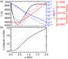 |
Fig. 1. Initial state of the simulations. Panel a: temperature (black), density (blue), and ionization fraction (red) of the atmosphere. Panel b: initial Lundquist number varying with height. The corresponding dashed lines represent the exact values in C7 model. |
We also assumed a uniform initial magnetic field:
 (18)
(18)
 (19)
(19)
 (20)
(20)
where c0 and b0 are constants. We chose c0 = 0.5 and b0 = 600 G for Cases 5, 5a, 5b, and c0 = 1 and b0 = 500 G for other cases.
Based on the initial temperature and ionization fraction of our simulations, we find that the initial η is in the order of 104 m2 s−1 in the whole simulation domain. We also estimated the corresponding Lundquist number LvA/η, where L = 1 Mm is the typical length scale of the system and  is the Alfvén speed. The initial Lundquist number is also shown in Fig. 1, and has values from ∼106 to ∼109. These values significantly exceed the critical Lundquist number (103 ∼ 104) for the onset of plasmoid instability (e.g., Bhattacharjee et al. 2009; Huang & Bhattacharjee 2010; Ni et al. 2013; Leake et al. 2012, 2013).
2.3. Boundary conditions
We used outflow boundaries at the top boundary. The fluid is only allowed to flow out of the computation domain by assuming:
where vyug and vyul separately represent the velocities at the two top ghost layers and at the last two layers inside the simulation box in the y-direction. The gradients of velocities in the x-direction and z-direction vanish at the top boundary by assuming  ,
,  . Similarly, the gradients of the thermal energy, mass density, and parallel components of magnetic field are set to zero. The perpendicular component of the magnetic field is obtained by divergence-free extrapolation of the magnetic field. We set the dynamic viscosity coefficient
 ![Mathematical equation: $ \nu = 10^4 \rho [1+10(1+\mathrm{tanh}\frac{\mathit{y}-1.95L_0}{0.1L_0})] $](/articles/aa/full_html/2021/02/aa39239-20/aa39239-20-eq28.gif) to make an enhancement of viscous diffusion around the top boundary.
to make an enhancement of viscous diffusion around the top boundary.
To drive the reconnection, we mimicked a flux emergence process similar to Ni et al. (2017) by setting the magnetic fields at the bottom boundary as:
![Mathematical equation: $$ \begin{aligned} B_{xb}&= \left\{ \begin{matrix} -0.85b_{0}+b_{1}\frac{\left( { y}-{ y}_{0} \right)L_{0}^{1.6}t}{\left[ x^{2} +( \left( { y}-{ y}_{0} \right)^{2} \right]^{1.3}t_{0}},&\ t\leqslant t_{0}\\ -0.85b_{0}+b_{1}\frac{\left( { y}-{ y}_{0} \right)L_{0}^{1.6}}{\left[ x^{2} +( \left( { y}-{ y}_{0} \right)^{2} \right]^{1.3}},&\ t> t_{0} \end{matrix}\right. \end{aligned} $$](/articles/aa/full_html/2021/02/aa39239-20/aa39239-20-eq29.gif) (21)
(21)
![Mathematical equation: $$ \begin{aligned} B_{{ y}b}&= \left\{ \begin{matrix} -0.35b_{0}-b_{1}\frac{xL_{0}^{1.6}t}{\left[ x^{2} +( \left( { y}-{ y}_{0} \right)^{2} \right]^{1.3}t_{0}},&\ t\leqslant t_{0}\\ -0.35b_{0}-b_{1}\frac{xL_{0}^{1.6}}{\left[ x^{2} +( \left( { y}-{ y}_{0} \right)^{2} \right]^{1.3}},&\ t> t_{0} \end{matrix}\right. \end{aligned} $$](/articles/aa/full_html/2021/02/aa39239-20/aa39239-20-eq30.gif) (22)
(22)
 (23)
(23)
where t0 = 60 s. The emerging flux and the greatest heights it can reach increase monotonically with y0 and b1. The divergence-free condition of the magnetic field in the simulation domain is satisfied. We chose y0 = −3 × 10⁵ m and b1 = 500 G for all the cases except Cases 5, 5a, and 5b. We set y0 = −2 × 10⁵ m and b1 = 600 G in Cases 5, 5a, and 5b so that the emerging flux reaches greater heights. The emerging magnetic field with such a form leads to reconnection magnetic fields in the (x, y) plane around the temperature minimum region of about several hundred Gauss. The small-scale flux emergences with a maximum strength of several hundred Gauss are frequently observed in reconnection events of UV bursts and EBs (e.g., Wang et al. 2020; Chen et al. 2019a), and much stronger magnetic fields of over several thousand Gauss have also been observed in active regions (e.g., Getling & Buchnev 2019; Liu et al. 2020; Leenaarts et al. 2018; Yan et al. 2017, 2020). Therefore, the strength of reconnection magnetic fields in our simulations is reasonable.
The fluid velocity was set to zero, and the density and thermal energy were fixed with the initial values at the bottom boundary. In addition, periodic boundary conditions were used in the horizontal direction.
3. Results and discussions
We tested ten different simulation cases, as summarized in Table 1. As mentioned before, we used a maximum AMR level of 1, 3, 5, and 7 in Cases 1, 2, 3, and 4, respectively. Radiative cooling, heat conduction, and ambipolar diffusion are all included in these cases. The effects of increasing spatial resolution are studied based on these cases.
Differences among simulation cases.
Then we turned off the radiative cooling, heat conduction, and ambipolar diffusion in Cases 3a, 3b, and 3c, respectively, to investigate the roles of different terms in our simulations; the highest refinement level in these cases is 5. We also ran cases (Case 5, 5a, 5b) with larger emerging flux. In Cases 5 and 5a, the maximum AMR refinement level is 5 and 3 respectively, but excluding ambipolar diffusion and heat conduction. The maximum AMR refinement level in Case 5b is also 3, but ambipolar diffusion is included.
3.1. Simulations with different spatial resolution
We started our simulations at relatively low resolution in order to obtain a general view of the magnetic reconnection processes. The maximum AMR level in Case 1 is 1, giving a minimum grid size of ∼2.86 km. The resolution in Case 1 is the lowest among all the Cases presented in this work, but it is still higher that those in previous 3D simulations in the low solar atmosphere (e.g., Hansteen et al. 2019). Four snapshots of Case 1 are presented in Fig. 2. The original data calculated using the NIRVANA code are transformed to uniform IDL data. First, the new emerging flux rises from the bottom boundary to the computation domain. The emerging flux interacts with the existing overlaying magnetic field, and a current sheet forms along the separatrice. The current sheet is filled with dense low-photosphere plasmas with a density that is larger than the ambient density. The temperature inside the current sheet is not heated above 10 000 K. As the current sheet continues to rise to a higher location, and plasmoids start to appear after it reaches 0.5 Mm above the solar surface. At the same time, the mass density in the current sheet decreases because the plasma is ejected to the exhaust region and then drops back because of gravity. The density and temperature distributions along the current sheet become nonuniform after the plasmoids appear. The cores of these plasmoids fill with dense photosphere plasmas and the plasmas at the edges of the plasmoids are usually more tenuous (see Fig. 3), especially when they are growing to bigger ones. Therefore, these regions with lighter plasmas are heated to higher temperatures (> 20 000 K). Later on, the plasmoids are ejected to the exhaust regions and the current sheet continues to rise. In the end, an oblique current sheet extends from 0 to 1.2 Mm in height and the mass density at the higher part of the current sheet is much lower than that at the lower part of the current sheet. Plasma at greater heights of the current sheet is heated to ∼105 K, while the temperature at lower heights of the current sheet is below 104 K. Such a final stage in Case 1 is similar to the results in Hansteen et al. (2019). In their 3D RMHD simulations, a vertical current sheet extends more than 2 Mm from the photosphere to the low corona, and the cool (< 104 K) and hot (≳105 K) plasmas are located at opposite ends of the current sheet.
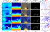 |
Fig. 2. General view of Case 1 with the lowest resolution. The distributions of temperature (a), density (b), total magnetic field strength (c), current density (d), and vertical velocity (e) at t = 226, 375, 569, and 611 s are presented. The white lines in the third column outline the magnetic field lines. The initial background magnetic field is about 500 G. |
Based on the results of Case 1, we increased the maximum AMR level step by step to investigate the effects of different computational spatial resolutions. In this work, we selected four cases with maximum AMR levels of 1, 3, 5, and 7, the comparisons among these cases are presented in Figs. 3 and 4. Increasing resolutions in the NIRVANA code shortens the time-step, which causes the runs with higher resolutions to be terminated earlier. However, the stages with plasmoid instability appearing in the reconnection region are well solved in all the cases. Fig. 3 presents the distributions of plasma temperature, density, and the joint probability distribution function (PDF) of temperature and density at a time after plasmoids appear in Cases 1 to 4. Figure 4 shows a zoom in to small scale in order to show the fine structures in one plasmoid. The Level-1 IDL data are used to plot Fig. 3, but the original levels of IDL data are used in Fig. 4.
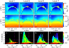 |
Fig. 3. Comparisons among Cases 1, 2, 3, and 4 with different maximum AMR levels, of namely 1, 3, 5, and 7, respectively. The distributions of temperature (panels a-d), density (panels e–h), and the joint PDF of temperature and density (panel i–l) at around 376 s are presented. The vertical and horizontal purple dashed lines in panels i–l indicate the positions with the density of 10−4.5 kg m−3 and the temperature of 2 × 10⁴ K. |
We find that the locations and morphologies of the current sheets in all four cases are similar. However, the fine structures inside the current sheets are very different. Plasmoid instability appears in Case 1, but only the big plasmoids of first order are identified. These big plasmoids are very smooth, and no turbulent structures appear inside them (see Figs. 3 and 4). More plasmoids appear in Cases 3 and 4, and the turbulent fine structures inside the big plasmoids as shown in Fig. 4 are only clearly observed in these two cases. The numerical results in Case 3 with level 5 AMR are similar to those in Case 4 with level 7 AMR. The density and temperature distributions in the reconnection region in Case 1 are also not uniform, but the differences among different components in Cases 3 and 4 are much larger and more obvious than those in Case 1, and more plasmas are heated to higher temperatures. Before the current sheet emerges above the middle chromosphere, the maximum temperature in the reconnection region in Case 1 is always below 30 000 K. Comparing Figs. 3 and 4, one can find the maximum temperature in the main current sheet reaches above 60 000 K in Case 2, and is about 50 000 K in Case 3 and 4. After the plasmoids are ejected out along the current sheet, they merge with the background plasmas and magnetic fields, both sides of the dome region become very turbulent and many fragment currents appear (see Fig. 5), especially on the right-hand side (see inside the black dotted box in Fig. 5). Figure 5 shows the results for Case 3: a turbulent reconnection outflow region is more clearly identified in the high-resolution runs, and the maximum temperature reaches about 80 000 K in this turbulent region in Case 3.
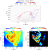 |
Fig. 5. Distributions of the current density in z direction (panel a), temperature (panel b) and the synthetic Si IV 1394 Å line emissions at each grid point (panel c) at a time during the later stage of the reconnection process in Case 3. The domain in panel b and panel c corresponds to the region in the dotted box in panel a. The black arrows in panel b represent the total velocity. |
In the simulations, both physical diffusion and numerical diffusion contribute to heating. Taking ohmic heating as an example, the heating rate Q can be written as Q = (η + ηnum)J2 = ηeffJ2, where ηnum is numerical diffusivity and ηeff is the total effective diffusivity. When the grid size becomes smaller, the current density increases and ηnum decreases. In Cases 1 and 2, the grids are coarse and the numerical diffusion dominates the heating. When the grid sizes become much smaller in Cases 3 and 4, the numerical diffusion becomes much less and the physical diffusion starts to play a role. Though the current density in Cases 3 and 4 is stronger than that in Case 2, the maximum temperature enhancement is less due to the smaller global ηeff. As shown in Figs. 3 and 4, the results in Case 3 are close to those in Case 4, which indicates that the simulation results in Case 3 and Case 4 are approaching the ones with realistic magnetic diffusion.
3.2. Effects of radiative cooling, heat conduction, and ambipolar diffusion
In order to understand the effects of radiative cooling in our simulations, we turned off radiative cooling and ran the simulation again to obtain Case 3a. Similarly, we dropped heat conduction and ambipolar diffusion in Cases 3b and 3c, respectively. The maximum AMR level in these Cases is 5, and we compared the results from Cases 3a, 3b, and 3c with those from Case 3 to study the three different effects on the magnetic reconnection process. The current sheet in these cases is not emerged to a location higher than 0.7 Mm before they are terminated because of the extremely small time-step. In order to check whether the ambipolar diffusion can effect the magnetic reconnection process at the greater height, we also tried to include this effect in Case 5. However, including the ambipolar diffusion effect in Case 5 leads to termination of the run before plasmoid instability appears. Therefore, we turned off the ambipolar diffusion effect in Case 5. We then performed another two simulations (Case 5a and 5b) using less refinements. The highest AMR level in Cases 5a and 5b is 3. The ambipolar diffusion is turned off in Case 5a and included in Case 5b. These results are presented in Figs. 6–8.
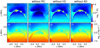 |
Fig. 6. Comparisons among Cases 3, 3a, 3b, and 3c where different terms are turned off in each. The distributions of temperature (panels a–d) and density (panels e–h) of cases 3, 3a (turning off radiative cooling), 3b (turning off heat conduction), and 3c (turning off ambipolar diffusion) are presented. |
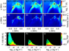 |
Fig. 7. Comparisons among three different cases. The distributions of temperature (panels a–c), total velocity the in x − y plane ( |

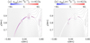 |
Fig. 8. Comparisons of two different energy terms at t = 403 s in Case 5b. Panel a: energy term emD contributed by effective magnetic diffusion, and panel b: energy term eAD contributed by ambipolar diffusion. |
Comparing the results of Cases 3 and 3a, one sees that radiative cooling plays an important role in such a magnetic reconnection process. Including radiative cooling makes plasmoids appear earlier (see Fig 6) and the dense cores of the plasmoids colder, which may significantly affect the synthesized spectral lines and images. Previous studies suggested that radiative cooling has little effect on the reconnection processes with a strong guide field (e.g., Uzdensky & McKinney 2011; Ni et al. 2015). However, the guide field in our models is quite strong (500 G) and the radiative cooling still plays an important. The mass density in the current sheet region in our simulations is larger than previous simulations, which is probably one of the reasons for such a discrepancy. Moreover, the reconnection process is driven by the strong flux emergence process in this work, which is different from the previous current sheet studies with small initial perturbations (e.g., Ni et al. 2015). We also find that the upper boundary is unrealistically heated to high temperatures where radiative cooling is excluded. Therefore, including radiative cooling is very important for numerical studies of activities in the low solar atmosphere. In this work, we used the radiative cooling model proposed by Gan & Fang (1990), in which the authors derived their model based on the detailed non-LTE calculations. Using the plasma parameters from the low solar atmosphere model (Vernazza et al. 1981), Gan & Fang (1990) found that the radiative loss calculated from their model is close to that from non-LTE calculations. Therefore, this model can provide a reasonable approximation of the radiative cooling in the photosphere and chromosphere. However, more realistic models and further studies are still necessary. Comparing Figs. 6a and c, one can find that heat conduction does not play a role in the main current sheet region. The maximum temperature ranges from several thousand to tens of thousands of Kelvin, which might mean that heat conduction along the magnetic field line is significant. However, the plasmoids with closed magnetic fields trap the heating within the plasmoids, and the heat conduction loses efficacy.
Previous studies showed that ambipolar diffusion can be very important in heating the chromosphere, and amplifying and transporting the magnetic tension (e.g., Khomenko & Collados 2012; Martínez-Sykora et al. 2017) in the low solar atmosphere. Our simulation results indicate that ambipolar diffusion does not significantly change the reconnection process and local plasma heating in the low chromosphere. Comparing Figs. 6a and d, one finds small differences in the details between Cases 3 and 3c. Fig. 7 also shows that the ambipolar diffusion effect causes the maximum temperature in Case 5b to be slightly higher than that in Case 5a. We calculated the two terms emD and eAD on the right-hand side of the energy equation at t = 403s in Case 5b with ambipolar diffusion, where ![Mathematical equation: $ e_{\mathrm{mD}}=\nabla \cdot \left [\frac{\eta_{\mathrm{eff}} }{\mu _{0}}\boldsymbol{B}\times \left ( \nabla \times \boldsymbol{B} \right )\right ] $](/articles/aa/full_html/2021/02/aa39239-20/aa39239-20-eq33.gif) and
and ![Mathematical equation: $ e_{\mathrm{AD}}=-\nabla \cdot \left [ \frac{1 }{\mu _{0}}\boldsymbol{B}\times \boldsymbol{E}_{\mathrm{AD}}\right ] $](/articles/aa/full_html/2021/02/aa39239-20/aa39239-20-eq34.gif) . The distributions of the two terms contributed by magnetic diffusion and ambipolar diffusion at this moment are presented in Fig. 8. We find that the maximum values of eAD and emD have about the same order of magnitude. As shown in Figs. 9c and d, the plasma density inside and around the current sheet region is ≳1020 m−3. Such a high plasma density causes the maximum ambipolar diffusion to be comparable to the maximum effective diffusion in our simulations. However, the areas with strong emD are much larger than the areas with strong eAD. The heating contributed by compression processes is also very strong. Therefore, the heating contributed by ambipolar diffusion is much less efficient compared to the other processes. As we zoom into the regions with strong eAD and emD, we also find that the locations with strong eAD are always staggered with the locations with strong emD. We should point out that the ionization fraction Yi is fixed in our simulations. As the realistic ionization fraction Yi should increase with temperature and the ambipolar diffusion ηAD decreases with increasing Yi and T, heating caused by ambipolar diffusion is possibly overestimated in our simulations. The ambipolar diffusion effect should become even less efficient than it is shown to be in this work if we consider the time-dependent ionization fraction. Ambipolar diffusion can possibly play important roles in the magnetic reconnection process above the middle chromosphere, where the plasma density is much lower. In recent work by Nóbrega-Siverio et al. (2020), the authors show that the ambipolar diffusion does not significantly change the amount of emerged magnetic flux when nonequilibrium ionization and recombination, and molecule formation of hydrogen are included, but it can efficiently heat the shock structures above the middle chromosphere.
. The distributions of the two terms contributed by magnetic diffusion and ambipolar diffusion at this moment are presented in Fig. 8. We find that the maximum values of eAD and emD have about the same order of magnitude. As shown in Figs. 9c and d, the plasma density inside and around the current sheet region is ≳1020 m−3. Such a high plasma density causes the maximum ambipolar diffusion to be comparable to the maximum effective diffusion in our simulations. However, the areas with strong emD are much larger than the areas with strong eAD. The heating contributed by compression processes is also very strong. Therefore, the heating contributed by ambipolar diffusion is much less efficient compared to the other processes. As we zoom into the regions with strong eAD and emD, we also find that the locations with strong eAD are always staggered with the locations with strong emD. We should point out that the ionization fraction Yi is fixed in our simulations. As the realistic ionization fraction Yi should increase with temperature and the ambipolar diffusion ηAD decreases with increasing Yi and T, heating caused by ambipolar diffusion is possibly overestimated in our simulations. The ambipolar diffusion effect should become even less efficient than it is shown to be in this work if we consider the time-dependent ionization fraction. Ambipolar diffusion can possibly play important roles in the magnetic reconnection process above the middle chromosphere, where the plasma density is much lower. In recent work by Nóbrega-Siverio et al. (2020), the authors show that the ambipolar diffusion does not significantly change the amount of emerged magnetic flux when nonequilibrium ionization and recombination, and molecule formation of hydrogen are included, but it can efficiently heat the shock structures above the middle chromosphere.
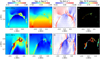 |
Fig. 9. Comparisons of the main current sheet region in Cases 3 (top panels) and 5 (bottom panels) at the times when the plasmoid instability is well developed. The distributions of temperature (panels a and b), density (panels c and d), vertical velocity Vy (panels d and f) are shown, along with the synthetic Si IV 1394 Å line emission at each grid point (panels g and h). The black arrows in panels e and f represent the total velocity. The background magnetic fields are 500 G and 600 G in Cases 3 and 5, respectively. The amount of emerging flux in Case 5 is greater than that in Case 3. The heat conduction and ambipolar diffusion effects are not included in Case 5. Panels g and h are shown in arbitrary units. |
3.3. Synthetic Si IV line profiles
We calculated the emissions and line profiles of the Si IV 1394 Å line of Case 3 and 5 based on the method described in Peter et al. (2006) using the atomic data package CHIANTI (version 9.0;Dere et al. 2019). Level 5 IDL data were used for calculations. First, we calculated the emissivity of the Si IV 1394 Å line at each grid point. The emissivity ε depends on density and temperature and can be written as:
 (24)
(24)
where ne is the electron number density and G(ne,T) is the contribution function which can be calculated from CHIANTI. Assuming that the line profile at each grid point has a thermal width of  , we calculated the spectral line profiles at each grid point with the unit of Doppler velocity:
![Mathematical equation: $$ \begin{aligned} I\left({ v}\right) = \frac{\varepsilon }{\sqrt{\pi }{ w}_{\rm th}}\exp { \left[-\frac{\left({ v}-{ v}_{0} \right)^{2}}{{ w}_{\rm th}^{2}} \right]} \end{aligned} $$](/articles/aa/full_html/2021/02/aa39239-20/aa39239-20-eq37.gif) (25)
(25)
where v0 is the component of velocity along the line of sight. Finally, we integrated the spectral line profiles over the whole region shown in Fig. 9 to obtain the total spectrum shown in Fig. 10.
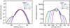 |
Fig. 10. Synthetic Si IV 1394 Å line profiles in Cases 3 and Case 5 taken along different lines of sight (left panel and right panel, respectively). The Si IV line profiles are integral over the whole region shown in the Fig. 9. Black, purple, blue, cyan, green, and red curves represent the line profiles taken along different lines of sight. The angles between the lines of sight and the vertical direction (y-direction) are 0°, 15°, 30°, 45°, 60°, and 75°, respectively. The dashed arrow represents the x-axis of the computation domain, and the solid arrows with different colors indicate the directions of lines of sight taken for calculating the Si IV line profiles shown with the same colors. |
In Case 3, we note that the hydrogen density within the current sheet is as large as 1021 m−3, and the emissions are underestimated because the Si IV has near-Saha-Boltzmann opacity and its formation temperature drops to 104 ∼ 2 × 10⁴ K at such a high density (Rutten 2016). However, there are still obvious Si IV emissions in the current sheet when using such a calculation method based on the optically thin assumption. The newly formed turbulent region also has strong emissions (see Fig. 5), and this region has a diameter of about 0.4 Mm. The stronger initial background magnetic field and emerged magnetic flux have been applied in the model to simulate Case 5. Comparing the results shown in Fig. 9, we find that the main current sheet with multiple plasmoids emerges to a higher location in Case 5, the plasmas are heated to much higher temperatures, and the maximum velocity is also higher in Case 5. The emission in the reconnection region in Case 5 is much stronger than that in Case 3 (see panels g and h of Fig. 9).
When the line of sight (LOS) is perpendicular to the direction of the reconnection outflow, the synthesized Si IV spectral profile is narrow and close to a single Gaussian profile (see the black solid lines in Fig. 10). As the LOS deviates from the direction perpendicular to the reconnection outflow, the doppler effect appears and the spectral line profile broadens and is no longer a single Gaussian profile. The multiple turbulent plasmoids along the LOS are the cause of the non-Gaussian line profile. However, the line width in Case 3 is only slightly broadened when the LOS passes through multiple plasmoids (see Fig. 10a). We find that the line width of the synthesized Si IV spectral line profile strongly depends on the maximum velocity along the LOS, which depends on both the local Alfvén velocity near the reconnection inflow region and the angle between the LOS and the reconnection outflow. Assuming that the strength of the reconnection magnetic field ranges from 200 to 2000 G, the corresponding plasma density is then between 4 × 10¹⁴ ∼ 1.6 × 10²¹ m−3 in order to obtain a local Alfvén velocity of 100 km s−1. Therefore, the reconnection region for generating the UV emissions with broad Si IV line width over 100 km s−1 should generally be located above the solar TMR. Our simulations in Case 5 with reconnection magnetic fields of ∼600 G show that the high-speed plasma that accounts for the broad Si IV line is located around 0.85 Mm above the solar surface (see Figs. 9b, d, f, and h). When the LOS is parallel to the direction of the maximum reconnection outflow velocity, the blue wing of the line profiles extends to about 100 km s−1. If the reconnection region is extended to a higher position or the reconnection magnetic field is stronger than that in Case 5, a broader line width can be generated.
UV bursts with small line widths have also been reported Hou et al. (2016), and their formation mechanisms are still unclear. Our simulations show that the narrow Si IV line profiles (see Fig. 10a) can easily form in the reconnection region around and above the solar TMR, as long as the reconnection magnetic fields are strong enough to cause the plasmas to be heated above 20 000 K. Compared to the UV bursts with broad line widths, the UV bursts with narrow line widths can be formed in a reconnection region at a lower height or with weaker reconnection magnetic fields (Fig. 10a), or the LOS direction and the reconnection outflow direction are almost perpendicular to each other (Fig. 10b).
4. Summaries, conclusions, and discussions
In this work, magnetic reconnection between the emerged and background magnetic fields is simulated to study the UV bursts found to be co-spatial and co-temporal with EBs. The strength of the reconnection magnetic fields with opposite directions is about several hundred Gauss after the current sheet reaches 0.5 Mm above the solar surface. The stratified atmosphere is close to the C7 model (Avrett & Loeser 2008). The initial temperature varies with height, and a temperature minimum region is included. Also, the plasma density changes more than five orders of magnitude from the bottom to 2 Mm above the solar surface. The partial ionization effect including ambipolar diffusion is considered in simulations. An empirical radiative cooling model based on observations is applied, and an anisotropic heat conduction is also included in our simulations. Simulations were performed by using different ARM levels, resulting in different resolutions in the current sheet region in different cases.
Our simulations can explain aspects of the formation of UV bursts. The hot tenuous plasmas and the cold dense plasmas carried upward from the photosphere are mixed up during plasmoid instabilities inside the reconnection region. The ejected plasmoids are then further merged into the background magnetic fields and plasmas, which causes the formation of the new turbulent region with many fragment currents. The temperatures in the plasmoids and in the new turbulent region can range from several thousand to about one-hundred thousand Kelvin, which could explain the different emission and absorption lines observed in a UV burst. The multiple turbulent structures along the LOS give rise to the non-Gaussian line profile of Si IV. However, the line width of the synthesized Si IV spectral line profile strongly depends on the maximum velocity along the LOS. The roundish shape of the plasmoids and the new turbulent region also closely agrees with the shape of UV bursts in observations (e.g., Peter et al. 2014; Tian et al. 2016; Chen et al. 2019b), which is different from the narrow elongated shape in the recent 3D simulations (Hansteen et al. 2019). Our simulations can also explain the association between UV bursts and EBs. The hot plasmas (> 20 000 K) inside the current sheet appear during the later stage of the reconnection process, which explains the fact that UV bursts are usually seen after their EB counterparts (Ortiz et al. 2020). The hot turbulent structures with strong Si IV emissions mainly appear above and around the solar TMR, and the cold plasma extends to much lower locations near the bottom of the current sheet at the solar surface (see Figs. 5 and 9). These phenomena are consistent with the observations that UV bursts tend to be observed at greater heights than corresponding EBs, and that EBs have partial overlap with their corresponding UV bursts in space.
Previous 2.5D simulations also showed the formation of plasmoids and the well-sythesized Si IV spectral line in a stratified solar atmosphere with flux emergence (e.g., Nóbrega-Siverio et al. 2016; Rouppe van der Voort et al. 2017). However, we should point out that plasmoids are formed above the upper chromosphere and the density in UV bursts is ≲1018 m−3 in those previous simulations (Nóbrega-Siverio et al. 2016; Rouppe van der Voort et al. 2017). The surface flows at the bottom boundary can also self-consistently drive the formation of the reconnection region of UV bursts (Peter et al. 2019). Instead of using a realistic density stratification, cases with different plasma densities were tested to study the effects of plasma β on generating UV bursts (Peter et al. 2019). The reconnection magnetic field in the simulations in Peter et al. (2019) is about 50 G, and the plasma with a density > 1019 m−3 is not heated above 20 000 K in their simulations. Observations suggest that the density of UV bursts is ≳1019 m−3 (Young et al. 2018); it could be even higher for those connecting with EBs (e.g., Tian et al. 2016). When the plasma β is the same, the temperature increase is much less in the plasma with a higher density in the lower atmosphere (Ni & Lukin 2018). Therefore, it is more difficult for plasmas to be heated to high temperatures above 20 000 K in the lower atmosphere. In this work, plasmoids are formed below the middle chromosphere, the density in UV bursts is about two to three orders of magnitude higher and reconnecting magnetic fields are also stronger than those in the previous models. Furthermore, the cool cores of the plasmoids and the multi-thermal turbulent fine structures inside the plasmoids and the reconnection outflow regions were not clearly shown in those previous simulations.
In the 3D simulations of Hansteen et al. (2019), the part of the long current sheet with Si IV emission extends downwardly to a position around the middle chromosphere. However, the plasmoid-like structures are not shown in their work. The hot and cool parts are basically located at opposite ends of a long current sheet (Hansteen et al. 2019). Ortiz et al. (2020) further proposed that the coexisting EBs and UV bursts could be part of the same reconnection system, even though they are located far apart on the vertical axis, which is different from the model in the present work. Though our results also show that the cold EB part extends to a lower height, the cold and hot plasmas could be concentrated in one plasmoid or the turbulent outflow region at about the same height. Priest et al. (2018) and Syntelis et al. (2019), Syntelis & Priest (2020) recently studied magnetic reconnection driven by photospheric flux cancelation. These authors pointed out that the hot and cool outflows produced without time difference and spatial offset are also found in a reconnection process without plasmoid-like structures.
A more realistic radiative-transfer process than that applied here has been well included in some of the previous simulations (e.g., Nóbrega-Siverio et al. 2016; Rouppe van der Voort et al. 2017; Hansteen et al. 2019) used to study UV bursts, but we have considered partial ionization effects and included the more realistic magnetic diffusion.
The simulations in this work have coupled the macroscopic scale of several Mm and the microscopic scale down to the ion inertial length (∼45 m), and both the observational features and the hidden small-scale physics are revealed. The results indicate that high-resolution simulations including realistic diffusivity in the stratified low solar atmosphere are essential for better understanding the magnetic reconnection mechanisms and plasma heating during the formation process of UV bursts. Obviously, low resolutions inevitably result in large numerical diffusivity and low Lundquist number. Large numerical diffusivity might result in unrealistic plasma heating in the reconnection region (as shown in Cases 1 and 2). Plasmoid instability will not appear if the Lundquist number is too low (e.g., Bhattacharjee et al. 2009; Ni et al. 2013; Leake et al. 2012), and the mixed hot tenuous and cold dense plasmas in the plasmoids and the turbulent reconnection outflow region will be smoothed out. This work qualitatively reveals the multi-thermal turbulent structures in the reconnection region of a UV burst. However, nonequilibrium ionization-recombination and more realistic radiative transfer in future simulations are needed to find the exact temperatures of the plasmas in these events. The obvious flux cancelations at the solar surface usually appear during the formation process of EBs and UV bursts (e.g., Peter et al. 2014; Tian et al. 2016; Chen et al. 2019b), which should also be included and discussed in future more realistic 3D simulations.
Acknowledgments
We thank Professor Rony Keppens for helpful discussions. This research is supported by the Strategic Priority Research Program of CAS with grants XDA17040507 and QYZDJ-SSWSLH012; the NSFC Grants 11973083; the Youth Innovation Promotion Association CAS 2017; the Applied Basic Research of Yunnan Province in China Grant 2018FB009; the Yunnan Ten-Thousand Talents Plan-Young top talents; the project of the Group for Innovation of Yunnan Province grant 2018HC023; the YunnanTen-Thousand Talents Plan-Yunling Scholar Project; the Special Program for Applied Research on Super Computation of the NSFC-Guangdong Joint Fund (nsfc2015-460, nsfc2015-463, the second phase); the Computational Solar Physics Laboratory of Yunnan Observatories; the Max Planck Partner Group program. Y.C. is supported by the China Scholarship Council for his stay in Germany. Y.J. and H.T. are supported by NSFC grants 11825301, 11790304(11790300), and the Max Planck Partner Group program.
References
- Archontis, V., & Hood, A. W. 2009, A&A, 508, 1469 [NASA ADS] [CrossRef] [EDP Sciences] [Google Scholar]
- Archontis, V., Moreno-Insertis, F., Galsgaard, K., & Hood, A. W. 2005, ApJ, 635, 1299 [NASA ADS] [CrossRef] [Google Scholar]
- Avrett, E. H., & Loeser, R. 2008, ApJS, 175, 229 [Google Scholar]
- Bhattacharjee, A., Huang, Y.-M., Yang, H., & Rogers, B. 2009, PhPl, 16, 112102 [Google Scholar]
- Braginskii, S. I. 1965, in Reviews in Plasma Physics, ed. M. A. Leontovich (New York: Consultants Bereau), 205 [Google Scholar]
- Chen, P.-F., Fang, C., & Ding, M.-D. 2001, Chin. J. Astron. Astrophys., 1, 176 [Google Scholar]
- Chen, Y., Tian, H., Zhu, X., Samanta, T., Wang, L., & He, J. 2019a, Sci. Chin. Technol. Sci., 62, 1555 [Google Scholar]
- Chen, Y., Tian, H., Peter, H., et al. 2019b, ApJ, 875, L30 [NASA ADS] [CrossRef] [Google Scholar]
- Chitta, L. P., Peter, H., Young, P. R., Huang, Y.-M., et al. 2017, A&A, 605, A49 [NASA ADS] [CrossRef] [EDP Sciences] [Google Scholar]
- Danilovic, S. 2017, A&A, 601, A122 [NASA ADS] [CrossRef] [EDP Sciences] [Google Scholar]
- De Pontieu, B., Title, A. M., Lemen, J. R., et al. 2014, Sol. Phys., 289, 2733 [NASA ADS] [CrossRef] [Google Scholar]
- Dere, K. P., Del Zanna, G., Young, P. R., et al. 2019, ApJS, 241, 22 [NASA ADS] [CrossRef] [Google Scholar]
- Ding, M. D., Hénoux, J.-C., & Fang, C. 1998, A&A, 332, 761 [Google Scholar]
- Ellerman, F. 1917, ApJ, 46, 298 [NASA ADS] [CrossRef] [Google Scholar]
- Fang, C., Tang, Y. H., Xu, Z., Ding, M. D., & Chen, P. F. 2006, ApJ, 643, 1325 [NASA ADS] [CrossRef] [Google Scholar]
- Fang, C., Hao, Q., Ding, M.-D., & Li, Z. 2017, Res. Astron. Astrophys., 17, 31F [Google Scholar]
- Galsgaard, K., Moreno-Insertis, F., Archontis, V., & Hood, A. 2005, ApJ, 618, 153 [Google Scholar]
- Gan, W. Q., & Fang, C. 1990, ApJ, 358, 328 [NASA ADS] [CrossRef] [Google Scholar]
- Georgoulis, M. K., Rust, D. M., Bernasconi, P. N., & Schmieder, B. 2002, ApJ, 575, 506 [NASA ADS] [CrossRef] [Google Scholar]
- Getling, A. V., & Buchnev, A. A. 2019, ApJ, 871, 224 [NASA ADS] [CrossRef] [Google Scholar]
- Grubecka, M., Schmieder, B., Berlicki, A., et al. 2016, A&A, 593, A32 [NASA ADS] [CrossRef] [EDP Sciences] [Google Scholar]
- Guglielmino, S. L., Young, P. R., & Zuccarello, F. 2019, ApJ, 871, 82 [NASA ADS] [CrossRef] [Google Scholar]
- Hansteen, V. H., Archontis, V., Pereira, T. M. D., et al. 2017, ApJ, 839, 22 [NASA ADS] [CrossRef] [Google Scholar]
- Hansteen, V., Ortiz, A., Archontis, V., Carlsson, M., Pereira, T. M. D., & Bjorgen, J. P. 2019, A&A, 626, A33 [NASA ADS] [CrossRef] [EDP Sciences] [Google Scholar]
- Heyvaerts, J., Priest, E. R., & Rust, D. M. 1977, ApJ, 216, 123 [NASA ADS] [CrossRef] [Google Scholar]
- Hong, J., Ding, M. D., & Cao, W. 2017, ApJ, 838, 101 [NASA ADS] [CrossRef] [Google Scholar]
- Hou, Z., Huang, Z., Xia, L., et al. 2016, ApJ, 829, 30 [NASA ADS] [CrossRef] [Google Scholar]
- Huang, Y.-M., & Bhattacharjee, A. 2010, PhPl, 17, 062104 [Google Scholar]
- Huang, Z., Mou, C., Fu, H., Deng, L., Li, B., & Xia, L. 2018, ApJ, 853, 26 [Google Scholar]
- Huang, Z., Li, B., & Xia, L. 2019, Sol.-Terr. Phys., 5, 58 [Google Scholar]
- Innes, D. E., Guo, L.-J., Huang, Y.-M., & Bhattacharjee, A. 2015, ApJ, 813, 86 [NASA ADS] [CrossRef] [Google Scholar]
- Isobe, H., Tripathi, D., & Archontis, V. 2007, ApJ, 657, 53 [Google Scholar]
- Khomenko, E., & Collados, M. 2012, ApJ, 747, 87 [NASA ADS] [CrossRef] [Google Scholar]
- Leake, J. E., Lukin, V. S., Linton, M. G., & Meier, E. T. 2012, ApJ, 760, 109 [NASA ADS] [CrossRef] [Google Scholar]
- Leake, J. E., Lukin, V. S., & Linton, M. G. 2013, PhPl, 20, 061202 [Google Scholar]
- Leenaarts, J., de la Cruz Rodríguez, J., Danilovic, S., Scharmer, G., & Carlsson, M. 2018, A&A, 612, A28 [NASA ADS] [CrossRef] [EDP Sciences] [Google Scholar]
- Lemen, J. R., Title, A. M., Akin, D. J., et al. 2014, Sol. Phys., 275, 17 [Google Scholar]
- Liu, H., Xu, Y., Wang, J., et al. 2020, ApJ, 894, 70 [NASA ADS] [CrossRef] [Google Scholar]
- Nelson, C. J., Scullion, E. M., Doyle, J. G., Freij, N., & Erdélyi, R. 2015, ApJ, 798, 19 [NASA ADS] [CrossRef] [Google Scholar]
- Martínez-Sykora, J., De Pontieu, B., Hansteen, V., et al. 2017, Sciences, 356, 1269 [Google Scholar]
- Murphy, N. A., & Lukin, V. S. 2015, ApJ, 805, 134 [NASA ADS] [CrossRef] [Google Scholar]
- Ni, L., & Lukin, V. S. 2018, ApJ, 868, 144 [NASA ADS] [CrossRef] [Google Scholar]
- Ni, L., Lin, J., & Murphy, N. A. 2013, PhPl, 20, 061206 [Google Scholar]
- Ni, L., Kliem, B., Lin, J., & Wu, N. 2015, ApJ, 799, 79 [NASA ADS] [CrossRef] [Google Scholar]
- Ni, L., Lin, J., Roussev, I. I., & Schmieder, B. 2016, ApJ, 832, 195 [NASA ADS] [CrossRef] [Google Scholar]
- Ni, L., Zhang, Q.-M., Murphy, N. A., & Lin, J. 2017, ApJ, 841, 27 [NASA ADS] [CrossRef] [Google Scholar]
- Ni, L., Lukin, V. S., Murphy, N. A., & Lin, J. 2018a, ApJ, 852, 95 [NASA ADS] [CrossRef] [Google Scholar]
- Ni, L., Lukin, V. S., Murphy, N. A., & Lin, J. 2018b, Phys. Plasmas, 25, 042903 [Google Scholar]
- Nóbrega-Siverio, D., Moreno-Insertis, F., & Martínez-Sykora, J. 2016, ApJ, 822, 18 [NASA ADS] [CrossRef] [Google Scholar]
- Nóbrega-Siverio, D., Moreno-Insertis, F., & Martínez-Sykora, J. 2018, ApJ, 8, 858 [Google Scholar]
- Nóbrega-Siverio, D., Moreno-Insertis, F., Martínez-Sykora, J., Carlsson, M., & Szydlarski, M. 2020, ApJ, 66, 633 [Google Scholar]
- Orrall, F. Q., & Zirker, J. B. 1961, ApJ, 134, 63 [NASA ADS] [CrossRef] [Google Scholar]
- Ortiz, A., Hansteen, V., Nóbrega-Siverio, D., & Rouppe van der Voort, L. 2020, A&A, 633, A58 [CrossRef] [EDP Sciences] [Google Scholar]
- Peter, H., Gudiksen, B. V., & Nordlund, Å. 2006, ApJ, 638, 1086 [NASA ADS] [CrossRef] [MathSciNet] [Google Scholar]
- Peter, H., Tian, H., Curdt, W., et al. 2014, Science, 346, 1255726 [Google Scholar]
- Peter, H., Huang, Y.-M., Chitta, L. P., & Young, P. R. 2019, A&A, 628, A8 [CrossRef] [EDP Sciences] [Google Scholar]
- Priest, E. R., Chitta, L. P., & Syntelis, P. 2018, ApJ, 862, 24 [Google Scholar]
- Romano, P., Elmhamdi, A., & Kordi, A. S. 2019, Sol. Phys., 294, 4 [NASA ADS] [CrossRef] [Google Scholar]
- Rouppe van der Voort, L., De Pontieu, B., Scharmer, G. B., et al. 2017, ApJ, 851, L6 [NASA ADS] [CrossRef] [Google Scholar]
- Rutten, R. J. 2016, A&A, 590, A124 [NASA ADS] [CrossRef] [EDP Sciences] [Google Scholar]
- Shibata, K., Nozawa, S., & Matsumoto, R. 1992, PASJ, 44, 265 [NASA ADS] [Google Scholar]
- Spitzer, L. J. 1962, Physics of Fully Ionized Gases (New York: Interscience) [Google Scholar]
- Syntelis, P., & Priest, E. R. 2020, ApJ, 891, 52 [NASA ADS] [CrossRef] [Google Scholar]
- Syntelis, P., Priest, E. R., & Chitta, L. P. 2019, ApJ, 872, 32 [NASA ADS] [CrossRef] [Google Scholar]
- Takasao, S., Isobe, H., & Shibata, K. 2013, PASJ, 65, 62T [Google Scholar]
- Tian, H., Xu, Z., He, J., & Madsen, C. 2016, ApJ, 824, 96 [CrossRef] [Google Scholar]
- Tian, H., Zhu, X., Peter, H., Zhao, J., Samanta, T., & Chen, Y. 2018a, ApJ, 854, 174 [NASA ADS] [CrossRef] [Google Scholar]
- Tian, H., Yurchyshyn, V., Peter, H., et al. 2018b, ApJ, 854, 92 [CrossRef] [Google Scholar]
- Uzdensky, D. A., & McKinney, J. C. 2011, PhPl, 18, 042105 [Google Scholar]
- Vernazza, J. E., Avrett, E. H., & Loeser, R. 1981, ApJS, 45, 635 [Google Scholar]
- Vissers, G. J. M., Rouppe van der Voort, L. H. M., & Rutten, R. J. 2013, ApJ, 774, 32 [NASA ADS] [CrossRef] [Google Scholar]
- Vissers, G. J. M., Rouppe van der Voort, L. H. M., Rutten, R. J., Carlsson, M., & De Pontieu, B. 2015, ApJ, 812, 11 [NASA ADS] [CrossRef] [Google Scholar]
- Vissers, G. J. M., de la Cruz Rodriguez, J., Libbrecht, T., et al. 2019, ApJ, 627, 101 [Google Scholar]
- Wang, J., Liu, C., Cao, W., & Wang, H. 2020, ApJ, 900, 84 [NASA ADS] [CrossRef] [Google Scholar]
- Watanabe, H., Vissers, G., Kitai, R., Rouppe van der Voort, L., & Rutten, R. J. 2011, ApJ, 736, 71 [NASA ADS] [CrossRef] [Google Scholar]
- Xue, Z., Yan, X., Cheng, X., et al. 2016, Nat. Commun., 7, 11837 [Google Scholar]
- Yan, X. L., Jiang, C. W., Xue, Z. K., et al. 2017, ApJ, 845, 18 [NASA ADS] [CrossRef] [Google Scholar]
- Yan, X., Xue, Z., Cheng, X., et al. 2020, ApJ, 889, 106 [NASA ADS] [CrossRef] [Google Scholar]
- Yang, H., Chae, J., Lim, E.-K., et al. 2013, Sol. Phys., 288, 39 [NASA ADS] [CrossRef] [Google Scholar]
- Yang, S., Zhang, J., Li, X., Liu, Z., & Xiang, Y. 2019, ApJ, 880, 24 [NASA ADS] [CrossRef] [Google Scholar]
- Yokoyama, T., & Shibata, K. 1995, Nature, 375, 42 [NASA ADS] [CrossRef] [Google Scholar]
- Young, P. R., Tian, H., Peter, H., et al. 2018, Space Sci. Rev., 214, 120 [NASA ADS] [CrossRef] [Google Scholar]
- Zhao, J., Schmieder, B., Li, H., et al. 2017, ApJ, 836, 52 [NASA ADS] [CrossRef] [Google Scholar]
- Ziegler, U. 2011, JCoPh, 230, 1035 [Google Scholar]
All Tables
All Figures
|
Fig. 1. Initial state of the simulations. Panel a: temperature (black), density (blue), and ionization fraction (red) of the atmosphere. Panel b: initial Lundquist number varying with height. The corresponding dashed lines represent the exact values in C7 model. |
| In the text | |
|
Fig. 2. General view of Case 1 with the lowest resolution. The distributions of temperature (a), density (b), total magnetic field strength (c), current density (d), and vertical velocity (e) at t = 226, 375, 569, and 611 s are presented. The white lines in the third column outline the magnetic field lines. The initial background magnetic field is about 500 G. |
| In the text | |
|
Fig. 3. Comparisons among Cases 1, 2, 3, and 4 with different maximum AMR levels, of namely 1, 3, 5, and 7, respectively. The distributions of temperature (panels a-d), density (panels e–h), and the joint PDF of temperature and density (panel i–l) at around 376 s are presented. The vertical and horizontal purple dashed lines in panels i–l indicate the positions with the density of 10−4.5 kg m−3 and the temperature of 2 × 10⁴ K. |
| In the text | |
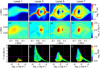 |
Fig. 4. Same as Fig. 3 but for a smaller field of view in one plasmoid taken around 352 s. |
| In the text | |
|
Fig. 5. Distributions of the current density in z direction (panel a), temperature (panel b) and the synthetic Si IV 1394 Å line emissions at each grid point (panel c) at a time during the later stage of the reconnection process in Case 3. The domain in panel b and panel c corresponds to the region in the dotted box in panel a. The black arrows in panel b represent the total velocity. |
| In the text | |
|
Fig. 6. Comparisons among Cases 3, 3a, 3b, and 3c where different terms are turned off in each. The distributions of temperature (panels a–d) and density (panels e–h) of cases 3, 3a (turning off radiative cooling), 3b (turning off heat conduction), and 3c (turning off ambipolar diffusion) are presented. |
| In the text | |
|
Fig. 7. Comparisons among three different cases. The distributions of temperature (panels a–c), total velocity the in x − y plane ( |
| In the text | |
|
Fig. 8. Comparisons of two different energy terms at t = 403 s in Case 5b. Panel a: energy term emD contributed by effective magnetic diffusion, and panel b: energy term eAD contributed by ambipolar diffusion. |
| In the text | |
|
Fig. 9. Comparisons of the main current sheet region in Cases 3 (top panels) and 5 (bottom panels) at the times when the plasmoid instability is well developed. The distributions of temperature (panels a and b), density (panels c and d), vertical velocity Vy (panels d and f) are shown, along with the synthetic Si IV 1394 Å line emission at each grid point (panels g and h). The black arrows in panels e and f represent the total velocity. The background magnetic fields are 500 G and 600 G in Cases 3 and 5, respectively. The amount of emerging flux in Case 5 is greater than that in Case 3. The heat conduction and ambipolar diffusion effects are not included in Case 5. Panels g and h are shown in arbitrary units. |
| In the text | |
|
Fig. 10. Synthetic Si IV 1394 Å line profiles in Cases 3 and Case 5 taken along different lines of sight (left panel and right panel, respectively). The Si IV line profiles are integral over the whole region shown in the Fig. 9. Black, purple, blue, cyan, green, and red curves represent the line profiles taken along different lines of sight. The angles between the lines of sight and the vertical direction (y-direction) are 0°, 15°, 30°, 45°, 60°, and 75°, respectively. The dashed arrow represents the x-axis of the computation domain, and the solid arrows with different colors indicate the directions of lines of sight taken for calculating the Si IV line profiles shown with the same colors. |
| In the text | |
Current usage metrics show cumulative count of Article Views (full-text article views including HTML views, PDF and ePub downloads, according to the available data) and Abstracts Views on Vision4Press platform.
Data correspond to usage on the plateform after 2015. The current usage metrics is available 48-96 hours after online publication and is updated daily on week days.
Initial download of the metrics may take a while.