| Issue |
A&A
Volume 646, February 2021
|
|
|---|---|---|
| Article Number | A87 | |
| Number of page(s) | 16 | |
| Section | Interstellar and circumstellar matter | |
| DOI | https://doi.org/10.1051/0004-6361/202038931 | |
| Published online | 11 February 2021 | |
Effects of anisotropy on absorption cross-section spectra of medium-sized spheroidal corundum particles
1
Leibniz Institute of Photonic Technology,
Albert-Einstein-Str.9,
07745
Jena,
Germany
e-mail: This email address is being protected from spambots. You need JavaScript enabled to view it.
; This email address is being protected from spambots. You need JavaScript enabled to view it.
2
Astrophysical Institute and University Observatory (AIU),
Schillergäßchen 2-3,
07745
Jena,
Germany
3
Institute of Physical Chemistry and Abbe Center of Photonics, Friedrich Schiller University,
Helmholtzweg 4,
07743
Jena,
Germany
Received:
15
July
2020
Accepted:
12
October
2020
Abstract
Context. It has been widely accepted that corundum particles condense in the atmospheres of oxygen-rich asymptotic giant branch stars and effectively produce an infrared emission feature at 13 μm. Laboratory experiments have predicted that these particles have the shape of oblate spheroids.
Aims. We investigate the influence of the material anisotropy of uniaxial corundum on absorption cross section spectra of medium sized spheroidal particles in the infrared spectral region.
Methods. We compared absorption cross-section spectra of the anisotropic corundum particles gained by finite-difference time-domain simulations to spectra calculated by a weighted sum approximation of the according fictive isotropic materials, with one material having the dielectric function of the a–b-plane and the other having the dielectric function of the c-axis of corundum. We carried out investigations for different axes ratios of the spheroids, particles volumes, and different geometries of the dielectric axes to the particle axes as well as to the polarization and propagation direction of the incident light.
Results. We observed several effects attributed to anisotropy that are non-additive, so that they cannot be reproduced with the combined spectra of the isotropic materials.
Conclusions. Care should be taken when calculating the corundum infrared spectrum with simpler approaches. When particle sizes above 1 μm are to be considered, the T-matrix formalism delivers correct band shifts and bulk modes for many, but not all bands. This remains true in orientation-averaged spectra and for particles in the 0.1 μm size range.
Key words: methods: numerical / dust, extinction / stars: AGB and post-AGB / astroparticle physics / solid state: refractory
© ESO 2021
1 Introduction
Early investigations of scattering behavior of ellipsoidal particles date back 70 yr. In 1951, the effects of the orientation of non-spherical particles on the interstellar reddening curve were investigated according to the idea that interstellar grains were non-spherical particles, oriented by magnetic fields (Davis & Greenstein 1951). In 1960, the first scattering cross-sections for arbitrarily oriented ellipsoids were approximately calculated in Greenberg & Meltzer (1960).
The total cross-sections of flattened ellipsoids were investigated for the propagation direction of the incident light parallel and normal to the major axis of the ellipsoid (Svatoš 1967). In 1977, in the work of Ruppin (1977) IR absorption spectra of spheroidal NaCl-crystallites were calculated with the point-matching method, taking into account, for the first time, retardation effects, so that bulk modes were at last included into the spectra. This allowed for the first investigation of particle-size effects on the spectra. In 1983, Bohren & Huffman (1983) published their famous text on the absorption and scattering of light by small particles, introducing the widely-used continuous distribution of ellipsoids (CDE) as a possible method for simulating wide particle shape distributions in the electrostatic limit (without retardation). A detailed study on the shape of interstellar grains with various CDEs can be found in Draine & Hensley (2017).
The first attempts to include the material anisotropy of ellipsoidal particles in the calculations date back to 1968, where the fields inside and outside small anisotropic dielectric ellipsoids are expanded in powers of the radius divided by the wavelength (Lysenko & Khizhnyak 1968). However, more sophisticated theories to treat anisotropic non-spherical materials could only be developed with increasing computational resources, such as Monzon (1989); Graglia et al. (1989); Papadakis et al. (1990). In 1965, the T-Matrix formalism was introduced by Waterman (1965), which, over the years, would turn out to be the most widely used formalism used to calculate scattering of electromagnetic waves on particles of all sorts of shapes and material properties (Mishchenko & Martin 2013). For a compilation of light scattering theories and corresponding computer codes1 we refer to Wriedt (2009), which covers both analytical and semianalytical methods as well as numerical methods.
The calculation of orientation-averaged spectra of (optical isotropic) ellipsoids to the T-matrix-formalism for non-spherical particles was implemented by Mishchenko, using an analytical averaging procedure (Mishchenko & Travis 1998; Mishchenko et al. 1996; Mishchenko 2001); we use this implementation later in this work. The T-matrix codes in Fortran90 have been extended to various scattering problems such as composite particles, layered particles, spheres with inclusions, particle clusters, and many more (Doicu et al. 2006; Schmidt & Wriedt 2009; Doicu 2003).
In spite of all the research done on the scattering of optically anisotropic particles, to the best of our knowledge, no frequency-dependent absorption, scattering, or extinction spectrum of an optically anisotropic ellipsoidal particle of a real material hasbeen calculated, nor have the actual effects of anisotropy on the spectra been systematically examined. In contrast, we find thatspectra of non-spherical particles, especially the astronomical spectra and spectra of astronomically relevant materials as in DePew et al. (2006); Pitman et al. (2013); Mutschke et al. (2013); Zeidler et al. (2013, 2015, 2011); Suto et al. (2006); Sturm et al. (2013); Takigawa et al. (2015); Bouwman et al. (2001); Tamanai et al. (2006a,b); Sogawa et al. (2006); Koike et al. (2010); Posch et al. (1999, 2007); Min (2009). This is due to the lack of better alternatives, whereby these spectra continue to be modeled with a variation of CDEs or limited distribution of ellipsoids (LDEs), or other similar formdistributions – and only in the electrostatic approximation (except for spheres). It is generally known that the averaging of spectra obtained by the individual crystallographic orientations of an anisotropic material is incorrect and leads, in some cases, to substantially erroneous band profiles, as shown in the example of forsterite in Mutschke et al. (2009). Furthermore, we showed in Höfer et al. (2020a,b) that no range of validity, as rule of thumb, can be given for the weighted sum approximation.
With the 13 μm emission feature observed in the asymptotic giant branch (AGB) star spectra, we have an example of an astronomically observed dust feature with a remarkably narrow spectral width, which excludes a broad shape distribution of the dust particles but, instead, points to a rather narrow form distribution. This is most likely produced by crystalline corundum particles (Takigawa et al. 2015; Zeidler et al. 2013), which predestines the material as model material for investigating spectral features caused by the optical anisotropy. The influence of the dust temperature and deviation from the spherical shape have already been thoroughly investigated (Takigawa et al. 2015; Zeidler et al. 2013) but so far relying only on the weighted sum approximation employing the electrostatic limit for the crystal optical anisotropy. Corundum grains can condense closer to the star than silicatedust particles due to the high thermal stability of aluminum oxide, that is, already at 1–2 stellar radii. Gobrecht et al. (2016) modeled in detail the condensation chemistry of aluminum oxide in the presence of pulsation-driven shocks in the inner winds of a Mira-type AGB star. Corundum grains with grain sizes between 0.5 and 5 μm formed in such AGB star atmospheres have been identified in primitive meteorites on Earth (Hoppe & Zinner 2000). Recently, Takigawa et al. (2018) presented strong evidence for the high-temperature condensation of a highly pristine presolar corundum grain around an AGB star.
In this work, we demonstrate the influence of (optical) anisotropy to the absorption cross-section spectra of spheroidal corundum particles from the results we obtained for a corundum sphere in a previous work. Furthermore, we give examples of how misleading the weighted sum approximation can be for the spheroidal corundum and we show that great care has to be taken in describing absorption spectra of corundum particles with the formalism of electrostatic approximation.
2 Simulation setups
The spectra of the uniaxial corundum particles were calculated with the commercial finite-difference time-domain (FDTD) software package Lumerical2. Since the FDTD is a time domain method, it allows us to cover a wide frequency or wavenumber range in a single simulation run and since the method discretizes the Maxwell equations in space, it treats anisotropic material properties in a natural way. The Lumerical software allows us to rotate the dielectric axes within the particle. In FDTD-simulations, the three-dimensional volume with the particle in the center is enclosed by a perfectly matched layer (the PML-box), which is a highly absorbing wall that allows the light to leave the simulation volume with minimal reflection (Gedney & Zhao 2010). Stacked around the particle,we have a six-sided box that records scattering, a six-sided total-field, scattered-field plane wave light source (Potter & Bérenger 2017; Taflove et al. 2013), and a box that monitors absorption. All required simulation parameters of Lumerical are listed in the Appendix. To generate the dielectric function, which is required for the FDTD simulations, we employed the oscillators parameters of corundum at 300 K provided by Zeidler et al. (2013).
In Höfer et al. (2020b), we investigated the influence of the material anisotropy on the absorption spectra of a corundum sphere for three different setups and for the spheroidal particles, we extended the investigations to nine different setups derived from the geometries of the sphere, as depicted in Fig. 1. For all setups, the light is incident parallel or normal to the axis of rotation symmetry of the spheroid, yet for a full study of orientation-dependent effects due to anisotropy, we would not only require the dielectric axes, but also the spectra of the particle itself tilted to the incident light. These orientations require a much larger volume of fine-grid resolution, which was beyond our computational resources. Nevertheless, as we show later on, the “missing orientations” are only important for larger axis ratios, approximately larger than 1:2.
For simplification, we describe the different geometries in Fig. 1 on the basis of the prolates: the left column shows the original setups that were employed for the sphere (see Höfer et al. 2020a,b). Provided that the incoming light remains parallel to one of the (physical) axes of the particle, the three setups of the sphere lead to nine different combinations of rotating the polarization direction of the incoming light or the dielectric tensor axes within the particle. The orientation of the spheroid is always with the symmetry axis in Z-direction. The polarization direction and the direction of the crystallographic axis (c-axis) are specified by the angles α and θ, respectively, in the way that α = 0° is always a polarization direction within the a–b-plane and θ = 0° means that the c-axis is normal to the propagation direction of the incident light.
In the first row of Fig. 1, the polarization direction of the incoming light is stepwise rotated, namely, it is always going from the a–b-plane for α = 0° to the c-axis for α = 90°. In setup 1_1p, the light is incident along the axis of rotation symmetry of the spheroids, the polarization is rotated from the X to the Y -axis, meaning that is goes from the a–b-plane for α = 0° to the c-axis for α = 90°; in setups 1_2p and 1_3p, the light is incident along the Y -axis of the FDTD-coordinate system; in setup 1_2p, the polarization direction is rotated from the X-axis (a–b-plane) to the Z-axis (c-axis); and in setup 1_3p the polarization direction is rotated from the Z-axis (a–b-plane) to the X-axis (c-axis).
In the setups of the second row, the orientation of dielectric axes with respect to the propagation and polarization direction of the incident light are altered in a way that the polarization direction remained in the a–b-plane3: in setup 2_1p, the light is incident along the axis of rotation symmetry, the dielectric tensor is rotated around the X-axis, so that the c-axis is normal to the propagation direction for θ = 0° and parallel to the propagation direction for θ = 90°. In setup 2_2p, the dielectric tensor is rotated in the same way, only the light is now incident along the Y -axis of the FDTD coordinate system.
For setup 2_3p, the propagation direction of the incident light remains along the c-axis (which is a short axis of the prolate and long axis for oblate particle), while the polarization direction of the incident light is rotated. Since the orientation of the c-axis to the propagation and polarization direction does not change here, setup 2_3p has only one reference spectrum of the sphere (the spectrum of setup 2, θ = 90°).
For the setups in the last row, the dielectric tensor axes are rotated in a way that the crystallographic axes get tilted to both the propagation and polarization direction of the incident light: At θ = 0°, the c-axis is always parallel to the polarization direction, which is oriented along the particle axis in setup 3_2p, while it is normal to it in setups 3_1p and 3_3p. At θ = 90°, the polarization is always in the a–b-plane.
To compare the spectra of the spheroidal particles to those gained for the spheres, we calculated the spectra for particles that have the same volume as a sphere with r = 1μm. In terms of the computation resources, we were limited to axis ratios4 not much larger than 1:4, of which we present the results for axis ratio 1:2 here to keep better track of the changes in the spectral features compared to the spectra of the sphere. The spectra for the axis ratio 1:4 can be found in Figs. A.1–A.3.
The spectral features originating from the optical anisotropy were identified by comparing the FDTD spectra to the (sum) spectra of hypothetical isotropic materials, having the dielectric function of only the a–b-plane or c-axis of corundum. To reduce the computational effort, the spectra of the isotropic materials were calculated with the T-matrix implementation SMARTIES from Somerville et al. (2016) instead of FDTD. The individual sum spectra were then calculated from weighted averages as summarized in Table 1. For instance, for setup 1_1p, the FDTD spectrum is modeled with the spectrum of a prolate having the dielectric function of the a–b-plane, the polarization direction of the incident light parallel to the short axis (named Cab,short), plus the spectrum of another prolate having the dielectric function of the c-axis and the polarization direction also parallel to the short axis. The terms cos2(α, θ) and sin2(α, θ) are the weighting factors taking into account the individual orientations of the polarization direction or the dielectric tensor axes. The FDTD spectra of setups 1_2p, 1_3p, 2_3p, 3_1p, 3_2p, and 3_3p (same setups for oblates) are modeled analogously to the spectra of setup 1_1p. For the remaining setups, for which the polarization direction is fixed in the a–b-plane, the FDTD spectra are modeled with the spectra of the hypothetical isotropic material having the dielectric function of the a–b-plane.
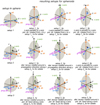 |
Fig. 1 Setups employed to investigate different orientations of the propagation and polarization direction of the incident light with respect to the dielectric tensor axes within the particle. The left column shows the setups employed for the spherical particle, the right side shows the setups resulting for the spheroidal particles (indexes “p” for prolate,“o” for oblate). For all setups, the axis of rotation symmetry of the particle is directed along the Z-axis of the FDTD coordinate system; either the directions of incidence and polarization, or the orientation of the dielectric axes within the particle are altered. |
Modeling the FDTD spectra of the anisotropic material with spectra of hypothetical isotropic materials.
3 Results
Figures 2–4, presenting the results for the spheroidal particles originating from the three setups of the sphere, are organized as follows: the left panels show the spectra of the prolate particle (setups labeled “p”), the right panels show the spectra of the oblate particles (setups “o”), and below these are the spectra of the corundum sphere from Höfer et al. (2020b) for comparison. The FDTD spectra, taking the material anisotropy fully into account, are presented in solid lines and the (sum) spectra of the fictive isotropic materials are given in dotted lines. For better representation, offsets were added to the spectra. The different orientations of the polarization and propagation direction of the incident light are color-coded: spectra for both the propagation and polarization direction of the incoming light parallel to the a–b-plane (α = 0°, θ = 0°) are in blue,the spectra for the polarization direction parallel to the c-axis (α = 90°, θ = 0°) in green. Spectra for the propagation direction parallel to the c-axis (θ = 90°) are in purple, the spectra of intermediate orientations are always in red (α, θ = 30°) and yellow (α, θ = 60°). Each blue, green, and purple spectrum occurs more than once in the three figures, as there are only three different configurations of each sort possible, specifically, for the three orientations of the spheroid symmetry axis. The only exception is the blue spectrum of setup 1_3p and 1_3o, which occurs only once. Instead, the purple spectrum in setup 3_3p,o occurs also in setups 2_2p,o and 2_3p,o (for α = 90°), that is, three times.
To simplify the discussion, we use consecutive numbers of the modes. Bands 1–6 are vibrational resonances in the a–b-plane and should thus dominate the blue and purple spectra, while bands 7–12 belong to the c-axis and should dominate the green spectra (however, see e.g., the appearance of the bulk modes 7 and 11 in setup 2p, o). Bands 2, 4, 7, 11 are bulk modes (Höfer et al. 2020b), while bands 3, 6, 10, 12 are the lowest order surface modes (Fröhlich-modes). Modes 1, 5, 8 are overlapped bulk and Fröhlich modes; here the oscillator strengths are too low to generate distinct bulk modes. Mode 9, which is excited for certain orientations, cannot be assigned to a surface nor a bulk mode, but it appears at the wavenumber position that corresponds to a reflection band in a bulk reflection spectrum and is, therefore, tentatively assigned to a reflection contribution. Bands 13 and 14 are higher-order surface modes, they exhibit more nodes in the components of the E-field (see Fig. B.1). Sole numbers refer to bands in the FDTD spectra, numbers with “a” to the according modes of the active isotropic materials.
Next, comparing the full FDTD simulation spectra with the weighted sum spectra derived from the isotropic calculations, we find in Figs. 2 and 3 (setups 1p, o and 2p, o) that the blue spectra presented for the two cases (solid and dotted) agree well with each other. It is only for the left slope of the strong modes 6 and 12 that there is a general discrepancy which is, however, due to the limitations of the FDTD grid; for this spectral region, we could not provide sufficient grid resolution and thus, the finer the grid, the smaller this discrepancy. The good agreement is obviously due to the fact that not only the polarization, but also the propagation directions are in the a–b-plane. Thus, a bending of the wave around the particle does not create any field components along the crystallographic c-axis and the isotropic calculations are sufficiently accurate for this case.
This does not remain true when the polarization direction is chosen along the crystallographic c-axis, that is, for the green spectra (see Fig. 2). Here, major differences occur with the bulk modes 7 and 11, which are shifted to higher (band 7), and, respectively, lower (band 11) wavenumbers compared to bands 7a and 11a resulting from the isotropic calculations. The shift distance depends on the particle shape. It is smallest for setups 1_2p and 1_1o, for which the c-axis is parallel to the long particle axis and the wave is incident along a short axis of the particle; while it is largest for setups 1_1p and 1_2o, where the opposite is true. As we showed in Höfer et al. (2020a), the bulk mode of an isolated oscillator gets shifted to higher wavenumbers, explaining the shift of band 7, while band 11 is strongly influenced by the bulk mode 4 at nearly the same wavenumber position.
An additional effect of the anisotropy is that the unsplit (overlapped) bulk and Fröhlich modes 1 and 5 of the a–b-plane (from the blue and purple spectra) remain present in the green spectra in all setups of Fig. 2, and also of Fig. 4, except for the setups where mode 5 becomes undetectable by the close approach surface mode 12 (setup 1_2p, setups 3_1o and 3_2p). Furthermore, several of the green FDTD spectra (for setups which produce a sufficient distance of bands 8 and 10) display an additional band (9), which we assign to a reflection feature (see above). Finally, the higher order surface mode 13 is visible for the setups that have the c-axis aligned to along particle axis (setup 1_2p, 1_3o, 1_1p only marginally) and is shifted to higher wavenumbers compared to band 13a of the isotropic material. The higher order mode 14 of the a–b-plane, if present in the blue spectra, is not shifted.
For the third class of spectra (the purple spectra), the crystallographic c-axis is now parallelto the incident wave propagation direction. As for the blue spectra, the incident electric field is always oriented in the ab-plane in this case. Thus, the isotropic spectra remain identical to the blue spectra, showing modes 1a to 6a. However, Fig. 3 clearly indicates that the purple FDTD spectra do not reproduce the bulk modes 2a and 4a, but show bands that are reminiscent of the shifted modes 7 and 11 of the green spectra (setups 2_1p, o and 2_2p, o, for θ →90°; setup 2_3, α = 0° and 90°). In all of the purple spectra, there is at most a minor feature remaining at the position of band 2a.
This is surprising as the transition dipole moments of the c-axis are not directly excited by the polarization direction of the incident wave. However, from Fig. 4 it becomes clear that these shifted bulk modes are indeed not (primarily) related to the a–b-plane (for an exemplary investigation of the E-field, see Figs. C.1 and C.2), as they result from a continuous shift of modes 7 and 11 of the green spectra by rotation of the c-axis from polarization direction into propagation direction (setups 3_1p, o and 3_2p, o). Consequently, the bulk modes 2 and 4 of the a–b-plane are obviously replaced by the bulk modes 7 and 11 of the c-axis, or possibly by combined modes 2/7 and 4/11, in the purple FDTD spectra.
The assumption that modes of different crystallographic axes combine in the spectra is further supported by the apparent coincidence of modes 3/8 and 13/14 into one band each in the setups of Fig. 4, including the sphere spectra. An analysis of the combined bands in the green and purple spectra shows that their positions depend mainly on the orientation of the c-axis, with respect to the particle symmetry axis, irrespective of whether it is parallel to the propagation or the polarization direction. As already discussed above for the green spectra, the combined modes occur at positions close to those of the c-axis modes (e.g., 7a and 11a) if c is aligned with a long particle axis and the other optical direction (propagation or polarization) is directed along a short particle axis. The opposite case leads to a combined mode close to the modes of the a–b-plane (e.g., 2a, 4a). Cases where both the c-axis and the other optical direction are oriented along equally long particle axes lead to intermediate band positions.
A rotation of the c-axis within the polarization or propagation plane thus leads to a shift of the band if the lengths of the associated particle axes are different (setups 3_1p, o, 3_2p, o). A rotation into the polarization or propagation plane leads to a shift with the rotation angle as well if the angle to the particle symmetry axis changes (setups 2_1, 2_2); the band then appears together with that of the a–b-plane mode until the c-axis is aligned with either of the two optical directions. If the c-axis rotates in the symmetry plane of the particle (setup 3_3p,o) or is fixed to the particle axes (setups 1, 2_3), there is no shift but a distinct position according the criteria in the previous paragraph.
Finally, concerning anisotropy effects for the lowest order surface modes, we observe a strong shift of mode 10 with respect to band 10a of the isotropic material for the intermediate rotation angles in setups 3_1p, o and 3_2p, o. This effect is not observed for the sphere, as it again depends on the particle geometry. For setups 3_2p and 3_1o (light incident along a short particle axis), band 10 is shifted to higher wavenumbers, whereas for setups 3_1p and 3_2o (light incident along a long particle axis), band 10 is shifted to lower wavenumbers compared to band 10a. A further effect on the Fröhlich modes is observed for bands 6 and 12, which for these setups have also merged into one, shifting band for these setups, while they appear overlapping but separate in the isotropic spectra.
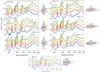 |
Fig. 2 Spectra of spheroidal corundum particles with axis ratio 1:2 of the setups derived from setup 1 of the sphere (bottom panel). Left panel: results for the prolate. Right panel: results for oblate particles. The FDTD spectra and combined spectra of the fictive isotropic materials are given in solid and dotted lines, respectively. Offsets were added to the spectra for better presentation. |
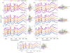 |
Fig. 3 Spectra of spheroidal corundum particles with axis ratio 1:2 of the setups derived from setup 2 of the sphere (bottom panel). Left panel: results for prolate. Right panel: results for oblate particles. Note that the spectra of setup 2_3 correspond to the sphere spectrum at θ = 90°. |
3.1 Influence of anisotropy on spectra of particle ensembles
As many experimental and, especially, astronomical spectra are measured on ensembles of arbitrarily oriented particles, we should now estimate how the anisotropy could affect orientation-averaged spectra. As, due to the computational and time effort, the number of FDTD spectra is limited, we take the average of the spectra for the orientations α, θ = 0,90° of the nine setups, for oblates and prolates, separately. As has already been pointed out, several of these are identical5, so that the average spectra are calculated with the nine independent FDTD spectra for each case (oblate, prolate).
Figure 5 presents the averaged spectra for oblates (above) and prolates (below) for particle volume equivalent of a sphere with r = 1 μm and axis ratio 1:2 (red colors) and 1:4 (blue colors). The average FDTD spectra are presented in solid lines (“av. FDTD”) and the average of the nine according spectra of the hypothetic isotropic materials are presented as dotted lines (“iso. mat.”). For comparison, we show the weighted sums (Cw.s.a = 1∕3 ⋅ Coa,c + 2∕3 ⋅ Coa,ab) of orientation-averaged spectra calculated for prolate (oblate) particles with the T-matrix formalism of Somerville et al. (2016) and the dielectric functions of the a–b-plane (Coa,ab) and the c-axis (Coa,c), respectively (“1/3.2/3.approx.”).
For the axis ratio 1:2, the dotted and thin gray lines agree very well with each other, except for the oblates around 800 cm−1, indicating that the choice of the nine spectra yields a very good approximation for an orientation-averaged spectrum. The influence of the material anisotropy becomes visible in the FDTD spectra between 400 and 440 cm−1, where there are several additional peaks in the latter one. At 570 cm−1 the two distinct peaks in the T-matrix spectra have moved closer together in the FDTD spectrum, with altered peak intensities.
For the axis ratio 1:4, the average of the nine spectra of the isotropic model materials (dotted lines) and the spectra of the 1/3–2/3-approximation (grey line) do not agree with each other between 650 and 720 cm−1 for the prolates; as for the oblates, there is only a small deviation at 770 cm−1. The additional peaks in the spectrum of the 1/3–2/3-approximation are absent in the other spectra due to the “missing orientation,” described in Sect. 3. The contribution of the missing orientations is proportional to sin2(45°) = 0.72, the maximum tilt angle, and becomes noticeable for larger axis ratios. Since the dotted and thin line for the rest of the spectral region agree with each other where they deviate from the averaged FDTD spectra, we can assign the material anisotropy to these deviations also. For the prolates, the extra peaks between 400 and 430 cm−1 and at 570 cm−1 get smoothed for the larger axis ratio; whereas for the oblates, there is barely a change if the particle gets flattened, the extra bands at 415 and 570 cm−1 remain practically unaltered.
With respect to the astronomical 13 μm (770 cm−1) feature, which we discuss in more detail in the next section, we note that the surface modes (6 and 12) dominating the spectrum in this wavelength region are strongly influenced by the particle shape. For oblates, two separate features to both sides of the original peaks (sphere) are produced. For the axis ratio 1:2, for instance, these are centered at 700 cm−1 (14.2 μm) and 820 cm−1 (12.1 μm), where the band at 700 cm−1 originates from spectra with polarization directions parallel to long spheroid axes and the band at 820 cm−1 from such with polarization along the short (symmetry) axis, both with sub-bands for the c-axis and a–b-plane optical constants. In contrast, the spectra of prolates have a main feature in the 750–800 cm−1 region (13.3–12.5 μm), shifting slightly to shorter wavelength with increasing spheroid axis ratio, while a less pronounced band is located at about 680 cm−1 or 14.7 μm (axis ratio 1:2) or even smaller wavenumbers. Thus, only prolate particles could roughly reproduce the 13 μm band for such elongated shapes.
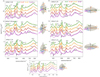 |
Fig. 4 Spectra of spheroidal corundum particles with axis ratio 1:2 of the setups derived from setup 3 of the sphere (bottom panel). Left panel: results for prolate. Right panel: results for oblate particles. |
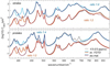 |
Fig. 5 Orientation-averaged spectra of oblate (upper panel) and prolate (lower panel) spheroidal particles with different axis ratios and equivalent sphere radius 1 μm. Solid lines: average of the 9 relevant FDTD spectra of the start- and endposition of each setup. Dotted lines: average of the according spectra of the isotropic materials. Thin grey lines: 1/3–2/3-approximation of the orientation-averaged spectra calculated with the T-matrix implementation of Somerville et al. (2016). For moderate axis ratios, the average of the nine spectra is a convenient alternative for an orientation-averaged spectrum. Thanks to this, the effects of the material anisotropy can be identified in the averaged FDTD spectra. |
3.2 Revisiting the 13 μm feature in astronomical spectra
Following Takigawa et al. (2015) and Zeidler et al. (2013), we turn now to less elongated spheroidal shapes (axis ratio around 1:1.4) and, in particular, to the oblate shapes predicted by experiments for corundum dust particles which condensed in the outflows of AGB stars. Neither the effects of particle sizes above the validity of the electrostatic approximation nor of the non-separability of crystal axes in such spectra have so far been studied with respect to the 13 μm emission band observed from these stars. For this purpose, we compare FDTD and T-matrix spectra similar to those in Fig. 5 – but this time for the oblate spheroid with axis ratio 1:1.4 – to the mean ISO SWS spectrum of 23 oxygen-rich AGB stars originally derived by Fabian et al. (2001) and also used by Zeidler et al. (2013).
For our calculations, we reduced the size of the particles as much as possible for the FDTD, that is, we choose an equivalent sphere radius of r = 0.75 μm, which is well within the size range reported for presolar corundum grains (Hoppe & Zinner 2000). The purple and the yellow lines in Fig. 6 represent the spectra analogous to these for the oblate particles in Fig. 5, that is, the average of nine FDTD spectra and the 1/3–2/3 sum of orientation-averaged TM spectra of the isotropic materials. While in the 13 μm region, the coincidence of these two is quite good, differences in the bands appear at around 17.5 μm (570 cm−1), 19.8 μm (505 cm−1), and in the 24–25 μm range (400–420 cm−1). While the first and the last of these deviations have already been discussed in the previous chapter as being signatures of the material anisotropy neglected in the isotropic calculations, the second was not noted there. The peak at 19.8 μm is present in Fig. 5 in both the FDTD and TM spectra and originates from polarization along the c-axis when parallel to the spheroid symmetry axis (setups 1_2o and 3_2o, green spectra). The reason this peak appears only as a weak shoulder in the T-matrix spectrum in Fig. 6 is not clear.
However, this difference remains present when we restrict the averaging to those spectra for which the c-axis is parallel to the short axis of the oblate spheroid, for instance, the two spectra with α = 0°, 90° of setup 1_2o.
This restriction corresponds to the finding of Takigawa et al. (2015), which states that corundum particles in AGB star atmospheres should be flattened along the c-axis. In this case, we compare the FDTD spectra, which have been averaged with 1/3 and 2/3 weights, respectively (red curve in Fig. 6), with the analogous average of the corresponding two single-orientation TM spectra (blue curve). Here, the 13 μm band complex has lost its side bands, apart from a shoulder at about 13.0 μm and peaks with the main band at 13.25 μm. The two individual spectra of the averaged FDTD-spectrum are shown in Fig. E.1, where it can be seen that the sharp peaks at 19.8 μm and 21 μm originate from the different polarization directions. A possible partial orientation or preferential orientation of the corundum particles might be observable in the ratio of these two peaks. The shoulder shows slight deviations between the FDTD and the isotropic spectrum. In the 17.5 μm band region,where the corresponding bulk modes (modes 4 and 11) are found, there remains a (somewhat structured) single feature at 17.5 μm in the FDTD spectrum, while the TM spectrum still shows two distinct bands. The surface mode 10 is now represented by a single band at 19.8 μm because the component for the c-axis oriented along a long particle axis has disappeared, but it is still significantly stronger in the FDTD spectrum than in the TM spectrum. A stronger feature in the FDTD spectrum is seen for bulk mode 2 as well (23.0 μm), while the overlapped bulk or surface mode band at about 25.9 μm is of similar strength in the two spectra. The strongest difference between the spectra calculated with the two methods is, again, the shift pattern of bulk mode 7 (here reduced to a single feature at 23.5 μm) with respect to “mode 7a” (25.3 μm) for the isotropic (T-matrix) result.
The main shortcoming of these simulations is the poor match of the position of the 13 μm feature withthe astronomically observed band. Thus, we calculate spectra for much smaller particles with the same geometries (here, because of the mentioned limitations of the FDTD, only with the TM method) and discuss changes in the spectra due to the particle size, as well as effects of a wider range of axis ratios. Figure 7 shows, again, the comparison of the astronomical spectrum (grey) with a spectrum calculated from orientationally averaged spectra of oblate particles with an axis ratio of 1:1.4 with isotropic dielectric functions (1/3–2/3-approximation, black dotted line), now for an equal-volume sphere radius of r = 0.1 μm. The main band is now peaking at about 13 μm and the bulk modes at 17.5 μm and in the 23–25 μm range have become too weak to be visible on the linear scale. Just as in the 13 μm band complex, the surface modes at 20–21 μm have slightly shifted to shorter wavelengths and the 19.8 μm shoulder is now a distinct peak but still rather weak (we recall that it was stronger in the FDTD spectra). The position of the weak (overlapped) modes 1 and 5 at 25.9 μm and 15.9 μm, respectively, is unaffected by the change in particle size (the apparent absence of bulk modes does not mean that they are necessarily undetectable in astronomical spectra). As Fig. 8 shows, bulk modes become more prominent already for corundum particles of radius 0.25 μm and larger. This should make it preferable to use theoretical models that include retardation effects, rather than the electrostatic approximation, for the simulation of dust emission spectra.).
The purple line demonstrates the effect of allowing for a larger range of axis ratios of 1:1.25–1:1.58, which we adopt from Takigawa et al. (2015, “LDE 1 - limited distribution of ellipsoidal shapes”). The main effect is an increase of the band width, especially in the 13 μm band complex, which produces a better fit to the astronomical feature, but also a slight increase of the band strengths in the 20–21 μm band region. If we omit again orientations of the dielectric tensor other than those with the c-axis parallel to the particle symmetry axis, we obtain the yellow dotted line for the axis ratio 1:1.4 and the red curve for the LDE 1. These curves show a very good agreement with the 13 μm main peak, the LDE 1 spectrum again having a somewhat broader band (see Takigawa et al. 2015), although we do not disregard the possibility that weak side bands originating from alternative orientations of the dielectric tensor might contribute to the astronomical feature.
We also found that a single orientation spectrum of an oblate with equivalent sphere radius of 1 μm (which is definitively out the electrostatic limit) in the orientation of setup 3_2o, θ = 90° matches the astronomical feature 13 μm equally well (blue line), as well as single orientation spectra of prolate particles with equivalent sphere radius 1 μm and axis ratio 1:2 (not shown). These coincidences point to the necessity of considering the bands appearing at longer wavelengths for the identification of the band carrier as, for instance, the blue spectrum shows the bulk modes at 17.6 and 23.5 μm, which clearly indicate large particles.
Sloan et al. (2003) found a clear correlation between the strengths of dust features at 13, 20 m and 28 μm (as well as with carbon dioxide bands) in AGB star spectra, which makes it possible that these bands arise from the same carrier. The 20 μm feature in question peaks on average at 19.8 μm and is equally broad as the 13 μm band (see Fig. 1 in Sloan et al. 2003). In contrast, our simulations of averaged spectra featuring a band at this position, which then originates from surface mode 10 with the c-axis being parallel to a short particle axis, is always accompanied by an at least equally strong band at 21 μm (surface mode 3). The single FDTD spectrum in Fig. 7 has a very strong peak at 19.8 μm but this peak is extremely sharp and additional bands would appear as soon as the particle or the dielectric tensor rotate. This makes it, in our opinion, rather unlikely that this feature also originates from corundum, but rather overlaps possible weaker corundum bands (see also Fig. D.1).
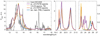 |
Fig. 6 Comparison of spectra calculated by T-matrix formalism (blue and yellow) and FDTD (red and purple) for spheroidal particles with axis ratio 1:1.4 and radius r = 0.75μm, showing spectral features due to material anisotropy. Grey line: mean of 23 measured ISO-SWS spectra. Purple line: average of nine FDTD spectra of the start- and endposition of each setup. Yellow line: 1/3–2/3-approximation of orientation-averaged spectra for two isotropic materials. Red line: average of the FDTD spectra (two of the three spectra are identical) calculated for the c-axis oriented parallel to the particle rotation axis. Blue line: the same for TM spectra |
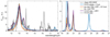 |
Fig. 7 Comparison of spectra calculated by the T-matrix formalism for oblate spheroidal particles of equivalent sphere radius 0.1 μmm (except blue line: r = 1μm) with the mean of 23 ISO-SWS spectra (grey line). Purple line: weighted sum of orientation-averaged spectra of spheroids of hypothetic isotropic materials, calculated for a limited distribution (LDE1) of axis ratios (1:1.25–1:1.58). Black dotted line: same, but for a sole axis ratio 1:1.4. Red line: average of the three spectra (two of them identical) with the c-axis parallel to the particle symmetry axis for the LDE1 axis ratio distribution. Yellow line: same for the sole axis ratio 1:1.4. Blue line: single FDTD spectrum of an oblate corundum particle with r = 1μm and ratio of 1:1.4. |
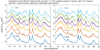 |
Fig. 8 1/3–2/3-approximations for an oblate corundum particle with ratio 1:1.4, equivalent sphere radius 0.1–1.5 μm, calculated including retardation effects (solid lines) and within the electrostatic approximation (dotted lines). |
4 Summary
We carried out a simulation of the FDTD spectra of anisotropic corundum particles in the IR spectral region for oblate and prolate shaped particles of different axis ratios and particle volume equivalent to that of a sphere with r = 0.75–1 μm. To identify the spectral features related to the material anisotropy, we compared the FDTD spectra to (sum) spectra calculated for two fictive materials with the dielectric function of the corundum c-axis and a–b-plane, respectively. The results demonstrate that the effects on the absorption spectra caused by the optical anisotropy depend very strongly on the considered geometry.
In the setups for the spheroidal particles derived from the sphere setup 1 (only the polarization is rotated), the FDTD spectra follow in general the transition from the spectrum of the a–b-plane to the spectrum of the c-axis, but with shifted bulk modes 7 and 11 compared to the modes 7a and 11a of the isotropic material and the appearance of bands 1 and 5 of the a–b-plane in the spectra with the polarization direction parallel to the c-axis. These shifted bulk modes are effects due to material anisotropy, the latter effect is a direct effect of the wave being bent around and penetrating into the particle.
In the geometries that were derived from the sphere setup 2 for two setups the dielectric tensor within the particle of the polarization direction was rotated in a way that the polarization remained in the a–b-plane, for another setup the polarization direction was rotated in the a–b-plane from a large to small particle axis, or vice versa. For these setups, bulk modes of the a–b-plane get replaced by bulk modes of the c-axis, although the transition dipole moments of the c-axis remain normal to the polarization direction. The bulk modes are now dependent of the applied rotation angle θ.
In the geometries derived from setup 3 of the sphere, if both the c-axis and a–b–plane get tilted to the particle surface and propagation and polarization direction of the incident light, bulk modes merge together to one band. Here, if the physical length spanned by the c-axis is changed with the rotation, also the strong surface modes 6 and 12 merge to one peak (setups 3_1p, 3_1o, 3_2p, 3_2o) and the position of the merged bands shift between the corresponding peak positions of the isotropic materials.
Depending on geometry, small peaks appear in the FDTD spectra, which have no counterpart in the spectra of the isotropic materials. Most probably, they originate from reflection contributions since they appear at wavenumber positions corresponding to reflection bands in bulk reflection spectra.
By modeling orientation-averaged spectra (Fig. 5), we show that for moderate axis ratios, the average of nine FDTD spectra of certain orientations between dielectric axes and propagation, and the polarization direction of the incident light is sufficient to calculate an orientation-averaged spectrum. This allows for the identification of spectral features related to anisotropy via a comparison to the corresponding averaged spectrum calculated from the fictive isotropic materials. For larger axis ratios, a wider range of orientations have to be taken into account.
Revisiting the 13 μm feature (Figs. 6 and 7) we found that not only the oblate corundum particles with the c-axis oriented along the short axis of the particle are suited to reproduce the 13 μm feature in observed ISO-SWS spectra, but also oblate particles with an arbitrarily oriented c-axis. The latter ones produce side peaks at 12.5 and 13.5 μm that might also be present in the astronomical spectra.
By investigating particle size effects, we can set upper limits to the particle size. The size of the corundum particles cannot be much larger than the size of the electrostatic limit (around r = 0.1μm), as, otherwise, the 13 μm-peak starts to shift to longer wavelengths. Taking into account a larger range of axis ratios around the center ratio 1:1.4 broadens the 13 μm band slightly, which gives a better fit to the astronomical spectra, but while still indicating that the shape distribution of the oblates is indeed quite narrow.
Nevertheless, it should not be overlooked that there are also some single-orientation spectra of oblate and prolate particles with sizes that are definitively outside the electrostatic limit, which also effectively reproduce the astronomical feature at 13 μm, providing hints that there might also be larger corundum particles. A final identification of the band carrier is only possible after obtaining additional information of the higher spectral region of 19–26 μm.
Acknowledgements
Our project has been supported by Deutsche Forschungsgemeinschaft, DFG under the grant HO 5868/1-1. We like to thank Simon Zeidler for providing the ISO-SWS spectrum.
Appendix A: Effect of material anisotropy on spheroids with larger axis ratios
Figure A.1 shows the result of the setups originating from setup 1 of the sphere for the axis ratio 1:4 for the prolate (left panel) and oblate particles (right panel), keeping the particle volume constant to that of a sphere with r = 1μm. As in the previous figures, the FDTD spectra that fully take into account the optical anisotropy of corundum are presented in solid lines and the spectra of the weighted sum approximation calculated from the fictive isotropic material are presented in dotted lines.
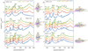 |
Fig. A.1 Spectra of spheroidal corundum particles with axis ratio 1:4 of the setups derived from setup 1. Left panel: results for prolate. Right panel: results for oblate particles. The FDTD spectra and combined spectra of the fictive isotropic materials are given in solid and dotted lines, respectively. Offsets were added to the spectra to improve the presentation. |
Concerning band 1 of the a–b-plane, which was present in all spectra of Fig. 2 throughout the rotation of the polarization direction α, this band has now almost entirely vanished for setups 1_2p and 1_1o as α approaches 90°. As the light is incident parallel to a short particle axis for these two setups, while the c-axis is oriented parallel to a long particle axis, the influence of the material anisotropy decreases as the prolate gets elongated or the oblate flattened. Band 5 of the a–b-plane is still persistent throughout the rotation in all setups for which the strong mode 12 does not overlap the wavenumber position of band 5. Theindividual changes of the spectral features compared to the lower axis ratio of Figs. 2–4are as follows.
In setup 1_1p for the axis ratio 1:4, there is no interplay between bands 2/7 and 4/11 of the FDTD spectra any more, however the interplay remains in the spectra of the isotropic materials. Here, bands 2/7 and 4/11 have merged into one band respectively, with the band position not depending on the polarization angle α, but fixed on the wavenumber position of bands 2a and 4a of the isotropic material.
In setup 2_2p, the bands in the FDTD spectra now follow the same transition from the spectra of the a–b-plane to the spectra of the c-axis except for a very slight shift between bands 7 and 7a for α → 90°. For setup 1_3p, the elongation of the prolate does not alter the effects due to anisotropy, the shift between bands 7/7a and 11/11a did not change for α → 90°, and, as for the ratio 1:2, band 9 is excited.
In setup 1_1o of the oblate particles, all FDTD spectra can very well be described with the weighted sum approximation, except for the small remaining shift between bands 7 and 7a, and a very small additional peak in the spectrum for α = 0° (circle). This peak is located at the wavenumber position of the reflection maximum in a bulk reflection spectrum.
For setups 1_2o and 1_3o, the flattening of the oblate has only little effect on the influence of the material anisotropy. For the first setup, the shift between bands 7/7a and 11/11a remains unchanged, but band 9 has moved to higher wavenumbers for the larger axis ratio and it is barely visible as a shoulder in band 10. For the latter setup, band 11 has moved to the same position as band 4. Band 13 has moved to the same position as band 14 and there is also no interplay between the corresponding bands in the spectra of the isotropic materials.
The spectra of the higher axis ratio for the setups derived from setup 2 of the sphere are presented in Fig. A.2. For the prolate particles, the general features caused by the material anisotropy do not change as the prolate gets elongated; for θ → 90° bulk modes 2 and 4 of the a–b-plane get replaced by bulk modes 7 and 11 of the c-axis, respectively. It is only for setup 2_3p, for which the propagation direction is fixed along the c-axis, where bands 2 and 4 have approached bands 2a and 4a of the isotropic material, so that for θ = 0° there is no longer any influence of the material anisotropy visible. The higher order surface mode 14 is no longer excited.
For the oblates, we observe a little more changes in the spectra as the particle gets flattened: in setup 2_1o all FDTD spectra agree now very well with the weighted sum spectra of the isotropic material, except for a marginal discrepancy at the positions of bands 2 and 4. This indicates that either the bulk modes 7 and 11 of the c-axis have moved to the same positions of bands 2 and 4, or that these modes of the c-axis do not contribute significantly any longer. Since in this setup the light is propagating parallel to the c-axis and is polarized to a four times longer particle axis in the a–b-plane, the latter option is much more likely. Encircled are small additional peaks, that are located at the wavenumber positions of reflection plateaus of bulk reflection spectra.
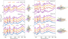 |
Fig. A.2 Spectra of spheroidal corundum particles with axis ratio 1:4 of the setups derived from setup 2. Left panel: results for prolate. Right panel: results for oblate particles. The FDTD spectra and spectra of the fictive isotropic material with the dielectric function of the a–b-plane of corundum are given in solid and dotted lines, respectively. Offsets were added to the spectra to improve the presentation. |
 |
Fig. A.3 Spectra of spheroidal corundum particles with axis ratio 1:4 of the setups derived from setup 3. Left panel: results for prolate. Right panel: results for oblate particles. The FDTD spectra and combined spectra of the fictive isotropic materials are given in solid and dotted lines, respectively. Offsets were added to the spectra for better presentation. |
For setup 1_2o, we observe that band 11 has moved closer to band 4 and the bulk modes 2a and 4a of the isotropic material are much less intense for θ → 90° than for the lower axis ratio. In contrast, the higher order surface mode 14 is much more intense. In setup 1_3o the wavenumber distance between bands 2/7 and 4/11 has increased by a few wavenumbers, and the higher order surface mode in both the FDTD spectra and spectra of the isotropic material is more intense.
The spectra of the geometries originating from the last setup of the sphere calculated for the higher axis ratio are shown in Fig. A.3. Compared to the axis ratio 1:2, there is only little change in the general spectral features caused by the material anisotropy.
Band 1 from the a–b-plane is persistent independently of the rotation angle θ for setups 3_1p, 3_3p, 3_2o and 3_3o, but not for setups 3_2p and 3_1o. For these latter two setups, the light is incident along a short particle axis and polarized parallel to the c-axis, which constitutes a four-times-longer particle axis. For θ = 90° there ism apart from a tiny shift between bands 2/7 and 7a, no influence of the material anisotropy. The arrows indicate simulation artifacts that would vanish for sufficient grid resolution6. For the intermediate rotation angles, there is still a strong shift between bands 10 and 10a, both shifted to somewhat lower wavenumbers, so that band 10a is only visible as shoulder in the band of 3/8.
In setups 3_1p and 3_2o, the angle-dependent shift of the position of band 2/7 has increased – for θ →90° it moves between the two positions of 2a and 7a of the isotropic materials, just as the combined band 4/11 already did for the lower axis ratio. Band 9 is not visible, but judging by the shift of the band to higher wavenumbers from ratio 1:1 (sphere) to ratio 1:2, it is now most probably overlapped by band 10.
For setup 3_3p, the elongation of the prolate did not influence neither the FDTD nor the spectra of the isotropic materials. This geometry is not affected by the elongation of the prolate since the propagation and polarization direction and the c-axis remain in the plane of equally long particle axes.
In setup 3_3o, for θ = 90° band 5 is overlapped by the intense mode 12 and a tiny additional peak appears (circle) at the position of a reflection band in a bulk reflection spectrum.
Appendix B: Higher order surface modes
Figure B.1 demonstrates that the absorption peaks 13 and 14 that are excited for various geometries are higher order surface modes, based on the example of setup 2_3p, α = 0°, ratio 1:2. The left side of the figure shows the slices through the mirror planes of the prolate at the lowest order surface peak 6 at 676 cm−1, while the right side shows the slices through the prolate at the position of peak 14 at 771 cm−1. All field components are normalized by their individual (absolute) maximal value, the number is given above each slice. Each field component for peak 14 exhibits more node points than do the field components for mode 6.
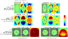 |
Fig. B.1 Demonstration of the higher order surface modes. |
Appendix C: Exemplarily investigation of the components of the E-field
Figure C.1 shows the components of the electric field for a prolate particle in the geometry of setup 2_3p, α = 0° (light incident along the c-axis, polarized along the long particle axis). The left side shows the components of the electric field for the axis ratio 1:2, while the right side shows the components for the axis ratio 1:4. For the ratio 1:2, the field components are shown for the absorption peak 2 at 426 cm−1; for the axisratio 1:4, the components are shown for the slightly shifted peak at 431 cm−1. The slices are cut through the three mirror planes of the prolate, while the polarization and propagation direction of the incident light with respect to the respective cut are given by the blue and pink arrows.
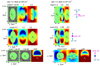 |
Fig. C.1 Exemplary investigation of the E field for setup 2_3p,α = 0°. |
To better compare the components of the E-fields to each other, the field component for each panel are normalized by their maximal (absolute) value, which is given above each panel. For this geometry, the influence of the optical anisotropy decreased as the prolate got elongated. In agreement with this observation, for the ratio 1:2, there is a distinct amount of E-field within the prolate in propagation direction (Ez component of X- and Z-cut) and in the top and bottom points of theprolate (Ey component of the X-cut). In the corresponding slices for the larger ratio, the magnitude of the field components within the particle is much lower, so for the smaller ratio, the wave penetrates more effectively into the particle than into the elongated prolate.
Figure C.2 shows the components of the electric field for a prolate particle oriented as in setup 2_3p, for α = 90° (light incident along the c-axis, polarized along the short particle axis). On the left side, we give the components of the electric field for the axis ratio 1:2 and on the right side, the components for the axis ratio 1:4 are presented. For both axis ratios, the field components are monitored at 417 cm−1.
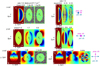 |
Fig. C.2 Exemplary investigation of the E field for setup 2_3p,α = 90°. |
For α = 90° the FDTD spectra showed no decreasing influence of the material anisotropy and in agreement with this observation, there is no general difference in the distribution of the field components in the particle for the two ratios. The Ex component has the same strengths and distribution in the X-cut and the three field components of the Y - and Z-cuts also have similar strength and distribution within the particle.
Appendix D: Similarity of single-orientation and orientation-averaged spectra
In Fig. D.1, we present a few more examples (see also Fig. 7) of single-orientation spectra with 13 μm band profiles that correspond to orientation-averaged spectra calculated with the electrostatic approximation for spheroids with certain axis ratios (Table D.1). The reason for those coincidences is that the high-intensity band of corundum between 11 and 15 μm stems from an almost threefold degenerate transition dipole moment, which allows for the same spectral shape for differently shaped particles. It is only for two FDTD spectra the oblate shape agrees with the particle shape in the electrostatic approximation, but not the axis ratios (spectra 2 and 4). The given axis ratio of the FDTD spectra agrees also twice with the axis ratio applied in the spectra of the electrostatic approximation, but here the particle shape does not agree (spectra 1 and 5). The spectral region in question of one FDTD spectrum agrees with a sphere spectrum of one fictive isotropic material. In all five examples the difference becomes only visible in the higher wavelength region.
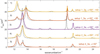 |
Fig. D.1 Colored solid lines: FDTD-spectra for single oblate particles with equivalent sphere radius r = 0.75 μm and axis ratio 1:1.4 for certain geometries. Dotted lines: orientation-averaged spectra calculated in the electrostatic limit. If only the band between 11 and 15 μm is considered, the spectra of the electrostatic approximation lead to erroneous interpretations. |
Appendix E: Addition to Fig. 6
Figure E.1 shows the two individual spectra of the oblate, which are employed to calculate the averaged spectrum in Fig. 6: in blue, we show the spectrum of the oblate with the polarization direction of the incident light parallel to the short axis and in red, the spectrum of the oblate with the polarization direction parallel to the long axis of the particle. While the spectral difference at around 13 μm might not necessarily be distinguished with a certain amount of noise added to the spectra, the sharp peaks at 19.8 and 21 μm are a characteristic feature created by the individual polarization directions. Information about this spectral region is crucial for further discussions of infrared spectra of corundum particles.
Appendix F: FDTD simulation parameters employed in Lumerical
The simulations were carried out with the Intel Xeon CPU E5-2680 v42.40 GHz 28 cores processor. The employed FDTD simulation parameters are as follows (a detailed explanation can be found in the online Lumerical handbook). Simulations were performed on a workstation with 28 dual core processors at 2.4 GHz and 128 GB RAM.
-
general FDTD parameters: background index = 1, simulation time 25ps, simulation Temperature 300 K. Power normalization to source intensity. To keep the simulation volume as small as possible and, at the same time, as large as necessary to minimize reflection from the PML boundary, the physical size of the simulation volume scales with of 18 times the short (long) radius in x–y directionand 18 times the long (short) radius in Z direction for prolate (oblate) particles
-
dt courant stability factor 0.99;
-
mesh accuracy = 3, mesh refinement: conformal variant 0;
-
using early shutoff (the simulation stops when the energy left in the system is lower than the given threshold), shutoff between 1e−9 and 1e−10, depending on geometry;
-
PML settings: stretched coordinate PML, standard profile with eight layers;
-
using mesh override, grid resolution scaled with particle shape so that smallest radius for both prolates and oblates was resolved with 25–40 grid points, depending on geometry;
-
monitor options: use source limits, no linear wavelength spacing, 1500 frequency points, 5–200 μm;
-
source options: set frequency/wavelength 5–200 μm, amplitude = 1.
References
- Bohren, C. F., & Huffman, D. R. 1983, Absorption and Scattering of Light by Small Particles (John Wiley & Sons) [Google Scholar]
- Bouwman, J., Meeus, G., de Koter, A., et al. 2001, A&A, 375, 950 [NASA ADS] [CrossRef] [EDP Sciences] [Google Scholar]
- Davis, Jr L., & Greenstein, J. L. 1951, AAS, 114, 206 [Google Scholar]
- DePew, K., Speck, A., & Dijkstra, C. 2006, ApJ, 640, 971 [Google Scholar]
- Doicu, A. 2003, Opt. Commun., 218, 11 [Google Scholar]
- Doicu, A., Wriedt, T., & Eremin, Y. A. 2006, Light Scattering by Systems of Particles (Springer, Berlin) [Google Scholar]
- Draine, B. T., & Hensley, B. S. 2017, ArXiv e-prints [arXiv:1710.08968] [Google Scholar]
- Fabian, D., Posch, T., Mutschke, H., Kerschbaum, F., & Dorschner, J. 2001, A&A, 373, 1125 [NASA ADS] [CrossRef] [EDP Sciences] [Google Scholar]
- Gedney, S. D., & Zhao, B. 2010, IEEE Trans. Antennas Propag., 58, 838 [Google Scholar]
- Gobrecht, D., Cherchneff, I., Sarangi, A., Plane, J. M. C., & Bromley, S. T. 2016, A&A, 585, A6 [NASA ADS] [CrossRef] [EDP Sciences] [Google Scholar]
- Graglia, R. D., Uslenghi, P. L. E., & Zich, R. S. 1989, Proc. IEEE, 77, 750 [Google Scholar]
- Greenberg, J. M., & Meltzer, A. S. 1960, AAS, 132, 667 [Google Scholar]
- Höfer, S., Mutschke, H., & Mayerhöfer, T. G. 2020a, JQSRT, 246, 106909 [Google Scholar]
- Höfer, S., Mutschke, H., & Mayerhöfer, T. G. 2020b, JQSRT, 256, 107241 [Google Scholar]
- Hoppe, P., & Zinner, E. 2000, J. Geophys. Res., 105, 10, 371 [Google Scholar]
- Koike, C., Imai, Y., Chihara, H., et al. 2010, ApJ, 709, 983 [Google Scholar]
- Lysenko, O. E., & Khizhnyak, N. A. 1968, Radiophys. Quant. Electron., 11, 311 [Google Scholar]
- Min, M. 2009, ASP Conf. Ser., 414, 356 [Google Scholar]
- Mishchenko, M. I. 2001, Appl. Opt., 39, 1026 [Google Scholar]
- Mishchenko, M. I., & Martin, P. A. 2013, J. Quant. Spectrosc. Radiat. Transfer, 123, 2 [Google Scholar]
- Mishchenko, M. I., & Travis, L. D. 1998, J. Quant. Spectrosc. Radiat. Transfer, 60, 309 [Google Scholar]
- Mishchenko, M. I., Travis, L. D., & Mackowski, D. W. 1996, J. Quant. Spectrosc. Radiat. Transfer, 55, 535 [Google Scholar]
- Monzon, J. C. 1989, IEEE Trans. Antennas Propag., 37, 728 [Google Scholar]
- Mutschke, H., Min, M., & Tamanai, A. 2009, A&A, 504, 875 [NASA ADS] [CrossRef] [EDP Sciences] [Google Scholar]
- Mutschke, H., Zeidler, S., & Chihara, H. 2013, Earth Planets Space, 65, 1139 [Google Scholar]
- Papadakis, S. N., Uzunoglu, N. K., & Capsalis, C. N. 1990, J. Opt. Soc. Am. A, 7, 991 [Google Scholar]
- Pitman, K. M., Hofmeister, A. M., & Speck, A. K. 2013, Earth Planets Space, 65, 129 [Google Scholar]
- Posch, T., Kerschbaum, F., Mutschke, H., et al. 1999, A&A, 352, 609 [NASA ADS] [Google Scholar]
- Posch, T., Baier, A., Mutschke, H., & Henning, T. 2007, ApJ, 668, 993 [Google Scholar]
- Potter, M., & Bérenger, J.-P. 2017, FERMAT, 19, 1 [Google Scholar]
- Ruppin, R. 1977, Surf. Sci., 62, 206 [Google Scholar]
- Schmidt, V., & Wriedt, T. 2009, J. Quant. Spectrosc. Radiat. Transfer, 110, 1392 [Google Scholar]
- Sloan, G. C., Kraemer, K. E., Goebel, J. H., & Price, S. D. 2003, ApJ, 594, 483 [Google Scholar]
- Sogawa, H., Koike, C., Chihara, H., et al. 2006, A&A, 451, 357 [NASA ADS] [CrossRef] [EDP Sciences] [Google Scholar]
- Somerville, W. R. C., Augié, B., & Le Ru, E. C. 2016, J. Quant. Spectrosc. Radiat. Transfer, 172, 39 [Google Scholar]
- Sturm, B., Bouwman, J., Henning, T., et al. 2013, A&A, 553, A5 [NASA ADS] [CrossRef] [EDP Sciences] [Google Scholar]
- Suto, H., Sogawa, H., Tachibana, S., et al. 2006, R. Astronom. Soc., 370, 1599 [Google Scholar]
- Svatoš. 1967, Bull. Astron. Inst. Czechosl., 18, 114 [Google Scholar]
- Taflove, A., Oskooi, A., & Johnson, S. 2013, Advances in FDTD Computational Electrodynamics: Photonics and Nanotechnology (Artech House, Inc.) [Google Scholar]
- Takigawa, A., Tachibana, S., Nagahara, H., & Ozawa, K. 2015, ApJ, 218, 2 [Google Scholar]
- Takigawa, A., Stroud, R. M., Nittler, L. R., Alexander, C. M. O., & Miyake, A. 2018, ApJ, 862, L13 [Google Scholar]
- Tamanai, A., Mutschke, H., Blum, J., & Meeus, G. 2006a, ApJ, 648, L147 [Google Scholar]
- Tamanai, A., Mutschke, H., Blum, J., & Meeus, G. 2006b, ApJ, 648, L147 [Google Scholar]
- Waterman, P. C. 1965, Proc. IEEE, 53, 805 [Google Scholar]
- Wriedt, T. 2009, J. Quant. Spectrosc. Radiat. Transfer, 110, 833 [Google Scholar]
- Zeidler, S., Posch, T., Mutschke, H., Richter, H., & Wehrhan, O. 2011, A&A, 526, A68 [NASA ADS] [CrossRef] [EDP Sciences] [Google Scholar]
- Zeidler, S., Posch, T., & Mutschke, H. 2013, A&A, 553, A81 [NASA ADS] [CrossRef] [EDP Sciences] [Google Scholar]
- Zeidler, S., Mutschke, H., & Posch, T. 2015, ApJ, 798, 125 [Google Scholar]
Freely available codes can be found at https://scattport.org/ and https://www.giss.nasa.gov/staff/mmishchenko/t_matrix.html
In Lumerical, the setting for α in setups 2_2p and 3_2p are 90° and 0°, respectively, but for a constant meaning of α in the figures we renamed it to α = 0, 90°.
To describe the shape of the spheroids, we employ the same definition as in Somerville et al. (2016). Here, the ratio is defined as the ratio between maximum and minimum distance from the origin, so the aspect ratio is always ≥1 for both prolate and oblate particles.
setup 1_1  setup 2_1
θ = 0°/ setup 1_1
setup 2_1
θ = 0°/ setup 1_1  setup 3_1
θ = 0°/ setup 1_2
setup 3_1
θ = 0°/ setup 1_2  setup 2_2
θ = 0°, setup 1_2
setup 2_2
θ = 0°, setup 1_2  setup 3_2
θ = 0°/ setup 1_3
setup 3_2
θ = 0°/ setup 1_3  setup 3_3
θ = 0°/ setup 1_3
α = 0°
has no equal, setup 2_1
setup 3_3
θ = 0°/ setup 1_3
α = 0°
has no equal, setup 2_1  setup 3_1
θ = 90°/ setup 3_2
setup 3_1
θ = 90°/ setup 3_2  setup 2_2
θ = 90°. setup 2_2
setup 2_2
θ = 90°. setup 2_2  both setup 2_3
α = 90°
and setup 3_3
θ = 90°.
both setup 2_3
α = 90°
and setup 3_3
θ = 90°.
Obviously, there are certain combinations of polarization angle and permittivity rotation for which the conformal mesh would not work and would therefore require a particularly fine grid (source: personal discussions with Lumerical Support).
All Tables
Modeling the FDTD spectra of the anisotropic material with spectra of hypothetical isotropic materials.
All Figures
|
Fig. 1 Setups employed to investigate different orientations of the propagation and polarization direction of the incident light with respect to the dielectric tensor axes within the particle. The left column shows the setups employed for the spherical particle, the right side shows the setups resulting for the spheroidal particles (indexes “p” for prolate,“o” for oblate). For all setups, the axis of rotation symmetry of the particle is directed along the Z-axis of the FDTD coordinate system; either the directions of incidence and polarization, or the orientation of the dielectric axes within the particle are altered. |
| In the text | |
|
Fig. 2 Spectra of spheroidal corundum particles with axis ratio 1:2 of the setups derived from setup 1 of the sphere (bottom panel). Left panel: results for the prolate. Right panel: results for oblate particles. The FDTD spectra and combined spectra of the fictive isotropic materials are given in solid and dotted lines, respectively. Offsets were added to the spectra for better presentation. |
| In the text | |
|
Fig. 3 Spectra of spheroidal corundum particles with axis ratio 1:2 of the setups derived from setup 2 of the sphere (bottom panel). Left panel: results for prolate. Right panel: results for oblate particles. Note that the spectra of setup 2_3 correspond to the sphere spectrum at θ = 90°. |
| In the text | |
|
Fig. 4 Spectra of spheroidal corundum particles with axis ratio 1:2 of the setups derived from setup 3 of the sphere (bottom panel). Left panel: results for prolate. Right panel: results for oblate particles. |
| In the text | |
|
Fig. 5 Orientation-averaged spectra of oblate (upper panel) and prolate (lower panel) spheroidal particles with different axis ratios and equivalent sphere radius 1 μm. Solid lines: average of the 9 relevant FDTD spectra of the start- and endposition of each setup. Dotted lines: average of the according spectra of the isotropic materials. Thin grey lines: 1/3–2/3-approximation of the orientation-averaged spectra calculated with the T-matrix implementation of Somerville et al. (2016). For moderate axis ratios, the average of the nine spectra is a convenient alternative for an orientation-averaged spectrum. Thanks to this, the effects of the material anisotropy can be identified in the averaged FDTD spectra. |
| In the text | |
|
Fig. 6 Comparison of spectra calculated by T-matrix formalism (blue and yellow) and FDTD (red and purple) for spheroidal particles with axis ratio 1:1.4 and radius r = 0.75μm, showing spectral features due to material anisotropy. Grey line: mean of 23 measured ISO-SWS spectra. Purple line: average of nine FDTD spectra of the start- and endposition of each setup. Yellow line: 1/3–2/3-approximation of orientation-averaged spectra for two isotropic materials. Red line: average of the FDTD spectra (two of the three spectra are identical) calculated for the c-axis oriented parallel to the particle rotation axis. Blue line: the same for TM spectra |
| In the text | |
|
Fig. 7 Comparison of spectra calculated by the T-matrix formalism for oblate spheroidal particles of equivalent sphere radius 0.1 μmm (except blue line: r = 1μm) with the mean of 23 ISO-SWS spectra (grey line). Purple line: weighted sum of orientation-averaged spectra of spheroids of hypothetic isotropic materials, calculated for a limited distribution (LDE1) of axis ratios (1:1.25–1:1.58). Black dotted line: same, but for a sole axis ratio 1:1.4. Red line: average of the three spectra (two of them identical) with the c-axis parallel to the particle symmetry axis for the LDE1 axis ratio distribution. Yellow line: same for the sole axis ratio 1:1.4. Blue line: single FDTD spectrum of an oblate corundum particle with r = 1μm and ratio of 1:1.4. |
| In the text | |
|
Fig. 8 1/3–2/3-approximations for an oblate corundum particle with ratio 1:1.4, equivalent sphere radius 0.1–1.5 μm, calculated including retardation effects (solid lines) and within the electrostatic approximation (dotted lines). |
| In the text | |
|
Fig. A.1 Spectra of spheroidal corundum particles with axis ratio 1:4 of the setups derived from setup 1. Left panel: results for prolate. Right panel: results for oblate particles. The FDTD spectra and combined spectra of the fictive isotropic materials are given in solid and dotted lines, respectively. Offsets were added to the spectra to improve the presentation. |
| In the text | |
|
Fig. A.2 Spectra of spheroidal corundum particles with axis ratio 1:4 of the setups derived from setup 2. Left panel: results for prolate. Right panel: results for oblate particles. The FDTD spectra and spectra of the fictive isotropic material with the dielectric function of the a–b-plane of corundum are given in solid and dotted lines, respectively. Offsets were added to the spectra to improve the presentation. |
| In the text | |
|
Fig. A.3 Spectra of spheroidal corundum particles with axis ratio 1:4 of the setups derived from setup 3. Left panel: results for prolate. Right panel: results for oblate particles. The FDTD spectra and combined spectra of the fictive isotropic materials are given in solid and dotted lines, respectively. Offsets were added to the spectra for better presentation. |
| In the text | |
|
Fig. B.1 Demonstration of the higher order surface modes. |
| In the text | |
|
Fig. C.1 Exemplary investigation of the E field for setup 2_3p,α = 0°. |
| In the text | |
|
Fig. C.2 Exemplary investigation of the E field for setup 2_3p,α = 90°. |
| In the text | |
|
Fig. D.1 Colored solid lines: FDTD-spectra for single oblate particles with equivalent sphere radius r = 0.75 μm and axis ratio 1:1.4 for certain geometries. Dotted lines: orientation-averaged spectra calculated in the electrostatic limit. If only the band between 11 and 15 μm is considered, the spectra of the electrostatic approximation lead to erroneous interpretations. |
| In the text | |
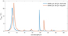 |
Fig. E.1 Two individual spectra of the averaged FDTD spectrum (red line in Fig. 6). |
| In the text | |
Current usage metrics show cumulative count of Article Views (full-text article views including HTML views, PDF and ePub downloads, according to the available data) and Abstracts Views on Vision4Press platform.
Data correspond to usage on the plateform after 2015. The current usage metrics is available 48-96 hours after online publication and is updated daily on week days.
Initial download of the metrics may take a while.