| Issue |
A&A
Volume 646, February 2021
|
|
|---|---|---|
| Article Number | A7 | |
| Number of page(s) | 15 | |
| Section | Stellar structure and evolution | |
| DOI | https://doi.org/10.1051/0004-6361/201937174 | |
| Published online | 29 January 2021 | |
Reinvestigating α Centauri AB in light of asteroseismic forward and inverse methods
1
STAR Institute, Université de Liège, Allée du 6 Août 19C, 4000 Liège, Belgium
e-mail: This email address is being protected from spambots. You need JavaScript enabled to view it.
2
Observatoire de Genève, Université de Genève, 51 Ch. des Maillettes, 1290 Sauverny, Switzerland
Received:
22
November
2019
Accepted:
9
November
2020
Abstract
Context. The α Cen stellar system is the closest neighbour to our Sun. Its main component is a binary composed of two main-sequence stars, one more massive than the Sun and one less massive. The system’s bright magnitude led to a wealth of astronomical observations over a long period, making it an appealing testbed for stellar physics. In particular, detection of stellar pulsations in both α Cen A and B has revealed the potential of asteroseismology for determining its fundamental stellar parameters. Asteroseismic studies have also focused on the presence of a convective core in the A component, but as yet without definitive confirmation.
Aims. Progress in the determination of solar surface abundances and stellar opacities have yielded new input for stellar theoretical models. We investigate their impact on a reference system such as α Cen AB. We seek to confirm the presence of a convective core in α Cen A by analysing the role of different stellar physics and the potential of asteroseismic inverse methods.
Methods. First, we present a new series of asteroseismic calibrations of the binary carried out using forward approach modelling and including updated chemical mixture and opacities in the models. We took advantage of the most up-to-date orbital solution as non-seismic constraints. We then complement our analysis with help of recent asteroseismic diagnostic tools based on inverse methods developed for solar-like stars.
Results. The inclusion of an updated chemical mixture -that is less metal-rich- appears to reduce the predicted asteroseismic masses of each component. Neither classical asteroseismic indicators such as the frequency ratios, nor asteroseismic inversions favour the presence of a convective core in α Cen A. The quality of the observational seismic dataset is the main limiting factor to settle the issue. Implementing new observing strategies to improve the precision on the pulsation frequencies would certainly refine the outcome of asteroseismology for this binary system.
Key words: asteroseismology / stars: solar-type / binaries: general / stars: oscillations
© ESO 2021
1. Introduction
The knowledge and characterisation of solar-type stars is a dominant subject of modern stellar physics. They are the best candidates to shelter planetary systems favourable to the development of life, while they are also key for a comparative study of the evolution and structure of our Sun. Solar-type stars can be precisely characterised as they exhibit pressure modes of pulsations, stochastically excited by near-surface convection. Interpreting the pulsations with asteroseismology provides tight constraints on the fundamental parameters of these stars and reveals their internal structure.
The CoRoT (Baglin et al. 2006) and Kepler (Borucki et al. 2010) space missions confirmed this potential, thanks to the data of unprecedented quality they delivered. This naturally benefited the study of solar-type stars (e.g., Metcalfe et al. 2012; Chaplin & Miglio 2013; Lebreton & Goupil 2014; Silva Aguirre et al. 2015; Buldgen et al. 2016a,b; Lund et al. 2017). Before this golden age for asteroseismology, exploitable detections of solar-like pulsations from the ground were only possible for a few stars (Bedding & Kjeldsen 2008). Among them, α Cen was and remains of particular interest for the study of solar-type stars. It is composed of two dwarf G- and K-type stars forming a binary system, of eccentricity e ∼ 0.52 and orbital period P ∼ 80 yr (Pourbaix & Boffin 2016), and a red dwarf, Proxima, thought to be gravitationally bound (Kervella et al. 2017a). The masses of the primary and secondary components are respectively estimated to MA ∼ 1.11 M⊙ and MB ∼ 0.94 M⊙ (Kervella et al. 2016). Consequently, the two stars are very similar to the Sun and are privileged targets for understanding the physics of solar-type stars. In particular, α Cen A is at the very limit in mass for the onset of convection in its nuclear-burning core. It thus represents an excellent testbed to the formalism of heat transport by convection, which remains a flaw of current stellar models.
As the closest stellar system to the Sun, the α Cen system presents bright apparent magnitudes of VA = 0.01 and VB = 1.33 (Ducati 2002), making it easier to perform a thorough analysis by numerous observing campaigns. Most were done for stellar physics purposes, resulting in a rich set of tight constraints on its stellar components, from exploiting the follow-up of their orbital motion (e.g., Wesselink 1953; Kamper & Wesselink 1978; Pourbaix et al. 2002; Pourbaix & Boffin 2016; Kervella et al. 2016) to determining their stellar atmospheres (e.g., Edvardsson 1988; Neuforge-Verheecke & Magain 1997; Bigot et al. 2008; Porto de Mello et al. 2008; Morel 2018). Renewed interest in the system came with the bloom of exoplanetology research. While the stability and existence of a habitable zone for exoplanets in the α Cen AB system has been theorised (e.g., Kaltenegger & Haghighipour 2013; Quarles & Lissauer 2016), claims for the detection of a planet orbiting α Cen B (Dumusque et al. 2012) have been dismissed (Hatzes 2013; Rajpaul et al. 2016) or await further evidence (Demory et al. 2015). Pursuing the characterisation of this system hence remains a crucial stake for stellar physics and the search for exoplanets.
A privileged approach is combining non-seismic and seismic information to constrain to the best level possible the fundamental parameters and the history of α Cen AB. Pulsations were expected to be present in the system components because of their similarity with the Sun. Before their observational detection was possible, the properties of putative α Cen stellar pulsations had thus already been studied (e.g., Edmonds et al. 1992; Kim 1999; Neuforge et al. 1999; Guenther & Demarque 2000). Alpha Cen A was the first solar-type star for which oscillations were detected from ground-based observations (Kjeldsen et al. 1999; Bouchy & Carrier 2001, 2002; Bedding et al. 2004) and from space by the WIRE spacecraft (Schou & Buzasi 2001; Fletcher et al. 2006). After the first asteroseismic modellings of α Cen A (Thévenin et al. 2002; Thoul et al. 2003), oscillations in α Cen B (Carrier & Bourban 2003; Kjeldsen et al. 2005) were also reported, opening the way to asteroseismic modelling of the binary system (e.g., Eggenberger et al. 2004; Miglio & Montalbán 2005; Yıldız 2007, 2008; Tang et al. 2008; Joyce & Chaboyer 2018). The first series of asteroseismic studies (Eggenberger et al. 2004; Miglio & Montalbán 2005; Yıldız 2007) showed a good agreement with masses obtained from the orbital solution and parallax estimate (e.g., Pourbaix et al. 2002) and interferometric radii (Kervella et al. 2003). Since then the picture of the system and stellar physics has evolved. Using longer observational runs, Pourbaix & Boffin (2016) revised their estimate of the masses of α Cen A and B by respectively about 3% and 5%. Between the first astero-seismic studies, important revision of the solar chemical composition (Asplund et al. 2005, 2009) and stellar opacities (Colgan et al. 2016) were also proposed. Moreover, several asteroseismic studies investigated whether α Cen A harbours a convective core (Miglio & Montalbán 2005; de Meulenaer et al. 2010; Bazot et al. 2012, 2016; Nsamba et al. 2018, 2019). None could firmly confirm its presence, and instead result in contradictory tendencies, depending on the asteroseismic dataset, namely suggesting no convective core in de Meulenaer et al. (2010), favouring one in Nsamba et al. (2019).
In this work we investigate the consequences on the asteroseismic modelling of recent developments in the physics of stellar models and check their consistency with the revised orbital solution of α Cen AB. We look at the impact of the metallicity scale of reference, which is generally the solar chemical mixture. The abundances of the elements that describe the solar mixture are derived mostly from the observation of the Sun’s photosphere. The measure of abundances from the photospheric spectra is not a side issue. For instance, Asplund et al. (2005, 2009) derived, using a new approach for the analysis of solar spectra, a severe decrease in the solar metallicity (∼30%) in comparison to previous works (e.g., Grevesse & Noels 1993). This modification of the metallicity reference itself will have an obvious impact on the internal properties of stellar models, in particular the opacity of the stellar plasma (e.g., Buldgen et al. 2019). The revision of the solar metallicity also led to a disagreement between theoretical models of the Sun and helioseismology (e.g., Bahcall et al. 2005). This solar issue raises the question of the accuracy of stellar physics ingredients of models, with particular concern for the opacity. In response, thorough numerical computations of opacity data for solar and stellar astrophysics were re-initiated (e.g., Mondet et al. 2015; Le Pennec et al. 2015; Colgan et al. 2016). In this framework we implement the recent Los Alamos opacities (Colgan et al. 2016) and assess whether asteroseismic calibrations of α Cen AB are sensible to the opacity changes.
The observational dataset of α Cen also benefited from new investigations. We take advantage of the asteroseismic dataset derived by de Meulenaer et al. (2010), which by combining multi-site observing campaigns has revealed the highest number and most precise oscillation frequencies to date of α Cen A. We hence calibrated a series of new models based on this frequency set and using Asplund et al. (2009) as the metallicity scale. We compared our results with the new orbital constraints from Pourbaix & Boffin (2016) and Kervella et al. (2016), and interferometric radii from Kervella et al. (2017b). The models, which are calibrated in a forward modelling approach, are then used as references to infer the presence of a convective core in α Cen A. We performed this with the help of asteroseismic inversions, based on the innovative framework developed in Buldgen et al. (2015, 2018). Our inversions are constructed to retrieve the entropy in the central layers of the stars, whose value behaves in a clear-cut way between the regime of convection or pure radiative transport.
We start by presenting in Sect. 2 the non-seismic and seismic constraints, and the input stellar physics we used for the asteroseismic calibrations of α Cen AB. Section 3 describes the calibration method by forward approach and recalls the basis for seismic inversion of the entropy. In Sect. 4 we present the results of our forward asteroseismic calibrations and discuss the impact on them of the revised metallicity scale of reference. In Sect. 5 we perform the seismic inversions and discuss their potential for assessing the presence of a convective core. We present our conclusions in Sect. 6.
2. Framework for asteroseismic calibrations of α Cen AB
2.1. Non-seismic observables
The α Cen AB orbital parameters were recently revised in two studies by Pourbaix & Boffin (2016, hereafter P16) and Kervella et al. (2016, hereafter K16), which are today the works of reference on this topic. As the system is a double-lined spectroscopic and visual binary, we can constrain from astrometry and spectroscopic radial velocities the total mass (MA + MB) and the fractional mass MB/(MA + MB), hereafter denoted by κ, of the system. With knowledge of the parallax, it is then possible to disentangle the individual masses. However, the parallax is a parameter adjusted to the same level as the fractional mass when solving the orbital system of equations (e.g., Pourbaix 1998). The individual masses in that approach are hence implicitly dependent on the other orbital parameters, both in P16 and K16. As noted by K16, the parallax determination of each team explains most of the differences between the individual masses determined by these two studies. We see in Table 1 that their values for κ differ by 0.6%, but rise to ∼3% for the individual masses. To avoid any dependence on the parallax derivation and its associated uncertainties, we adopt the fractional mass rather than the individual masses as observational constraints in most of our calibrations. The values of P16 and K16 for κ are very similar, and we only selected the K16 value because their analysis included a longer follow-up of the astrometric record.
Non-seismic observational parameters for α Cen AB.
The radius ratio RA/RB (denoted Γ) is obtained from angular diameters determined by interferometry and is an interesting parameter to exploit. It is indeed firmly constrained because of its independence of the wavelength band of the observation and of the parallax. From a new set of interferometric data, Kervella et al. (2017b) derived a value Γ = 1.4172 ± 0.0016, in perfect agreement with their earlier estimation (Kervella et al. 2003). We consequently chose it as the second observational constraints for our calibrations. Nevertheless, we also performed some with the individual radii and masses from Kervella et al. (2017b) and K16 (the same parallax is adopted in both studies) to analyse how they influence the results of our calibrations (see Sect. 4).
The system is well known for being metal rich (French & Powell 1971) and, owing to its brightness, it has motivated many spectroscopic studies of its stellar component atmospheres. Discrepancies exist between studies (see e.g. discussion in Porto de Mello et al. 2008), but most of the metallicity determinations of α Cen AB give a value for the system of [Fe/H] ∼ 0.25 (see the short review in Morel 2018). Used in the first series of asteroseismic studies, the reference values of Neuforge-Verheecke & Magain (1997) are in excellent agreement with more the recent determinations of Porto de Mello et al. (2008) and Morel (2018) (see Table 1). As in Neuforge-Verheecke & Magain (1997), the work of Porto de Mello et al. (2008) found a negligible difference between the A and B component metallicities. Therefore, we selected from these latter authors the single [Fe/H] = 0.24 value as the common present-day surface metallicity to be reproduced by our models for each component. Despite convergence between the different spectroscopic studies (based on 1D stellar atmosphere models), Bigot et al. (2008) found a departing value, [Fe/H] = 0.16, that they derived for α Cen A with 3D hydrodynamical simulations. Although the authors mention this work as preliminary, their value is intriguing and deserves to be considered. We also carry out some calibrations of the system using this lower metallicity value.
Effective temperatures (Teff) derived in the spectroscopic studies are in the ranges 5750 ≲ Teff, A ≲ 5850 K and 5150 ≲ Teff, B ≲ 5300 K for the A and B components (see review in Morel 2018). Based on the bolometric fluxes of the stars, Kervella et al. (2017b, and references therein) derived effective temperatures (see Table 1) in perfect agreement with the spectroscopic values. We choose their values as constraints because we also use the fractional mass and radius ratio derived by the same authors.
2.2. Seismic constraints
Oscillations in α Cen A were analysed by Bouchy & Carrier (2001, 2002) from a 13-night radial velocity dataset, resulting in the detection of 28 modes (with angular degrees ℓ = 0, 1, 2). Independently, Bedding et al. (2004) and Butler et al. (2004) observed the star for five nights, detecting 42 modes (ℓ = 0, 1, 2, 3). More recently, Bazot et al. (2007) detected 34 modes (ℓ = 0 − 3) from a new five-night run of observations. Notably, the datasets from Bouchy & Carrier (2002), Bedding et al. (2004) and Butler et al. (2004), were taken on overlapping dates in 2001, from multi-site facilities (in Chile and Australia). de Meulenaer et al. (2010), in an effort to combine those data, reduced the aliases induced by the day/night duty cycle. They obtained the most precise and complete set of acoustic oscillations for α Cen A, with 46 modes from ℓ = 0 to 3. For the frequency set of α Cen B, we adopt the richest one derived by Kjeldsen et al. (2005), consisting of 37 acoustic modes with ℓ = 0 to 3.
The oscillation frequencies can be combined to define seismic indicators sensitive to different stellar properties. We considered in particular the large and small differences of mode frequencies, Δνn, ℓ and δνn, ℓ, defined as
 (1)
(1)
and
 (2)
(2)
where νn, ℓ is the frequency of a mode of radial order n and angular degree ℓ. It is a good approximation to assume the acoustic oscillations of solar-like stars are in the asymptotic regime. In this regime it can be shown (e.g., Gough 2003) that these frequency differences approach constant values known as the large and small separations, which are proportional to structural stellar quantities. The latter is a proxy of the mean stellar density, the former depends on the gradient of sound speed, which is mostly sensitive to the chemical stratification in the stellar core.
When comparison to observations are made, particular care is required to retrieve these indicators from the theoretical models in a similar way. For instance, the observed large separations for α Cen are derived from the autocorrelation of the asymptotic formula to the oscillation spectra (e.g., Bouchy & Carrier 2002), which is hardly reproducible without bias from theoretical frequencies. Instead, we derived the observational large separation Δν from a linear fit to the individual frequencies (ν as a function of n) for each ℓ and n detected. We then computed the weighted mean of the four fitted values (ℓ = 0, 1, 2, 3), obtaining ΔνA = 105.9 ± 0.3 μHz and ΔνB = 161.4 ± 0.3 μHz, respectively for the A and B component. Uncertainties were taken as the standard errors of each estimate and then propagated. We implemented in our calibrations the calculation of the theoretical large separations similarly, i.e. from linear fits to the theoretical frequencies of the models, on the same ℓ and n as observed. For the small separation we worked with the arithmetic mean value of the small differences for ℓ = 0, δνn, 0, following the definition in Eq. (2). The observational values are then ⟨δν0, A⟩ = 5.63 ± 0.73 μHz and ⟨δν0, B⟩ = 10.90 ± 1.85 μHz. The theoretical values were computed similarly.
These two indicators are combined to constrain the mean density of solar-like oscillators and their evolutionary stage, but they can suffer a bias due to surface effects affecting the observed individual frequencies. A solution is to add surface effect corrective terms to theoretical frequencies (e.g., Kjeldsen et al. 2008). The form of the corrections and how they are computed are still a matter of intense debate. Another approach consists in defining seismic indicators as insensitive to surface effects as possible. Roxburgh & Vorontsov (2003) proposed to divide the small frequency separations by the large ones to break free from these effects:
 (3)
(3)
Here d10 is the five-point small separation, as defined in Eq. (5) of Roxburgh & Vorontsov (2003). These indicators are sensitive to variations in the chemical composition profile in the central stellar layers. They provide insightful information on the age and the physical conditions in the nuclear core. Their potential was tested in detail for α Cen A in Miglio & Montalbán (2005) and de Meulenaer et al. (2010) as posterior constraints. The r10 and r13 ratios seemed promising indicators of the energy transport process in the central layers, by showing a distinct behaviour between models of α Cen A with or without convective core. We pursued this effort by including indicators of Eq. (3) as a priori seismic constraints for a series of calibrations.
2.3. Physics of the models
Relying on the observational constraints described above, we computed all our numerical models with the Liège stellar evolution code (CLES, Scuflaire et al. 2008a). The treatment of convection follows the mixing-length prescription (Böhm-Vitense 1958), and is implemented following Cox & Giuli (1968). Except for some calibrations (see Table 2), no overshooting was considered. When included, overshooting is implemented as an instantaneous extra-mixing extending over a region whose size is αov × min[rcc, HP(rcc)], with rcc the size of the convective core, HP the local pressure scale height, and αov an overshooting parameter. The surface boundary conditions are obtained from Eddington’s law (T[τ], T being the temperature) for a grey atmosphere, with the atmosphere extended down to an optical depth τ ∼ 10−6. The nuclear reaction rates were those of the Nacre (for nuclei with atomic mass A > 15) and Nacre-II (A < 16) compilations (Angulo et al. 1999; Xu et al. 2013), with the exception of the two first reactions of the pp-I chain whose rates were taken from Adelberger et al. (2011). We adopted the updated solar chemical mixture of Asplund et al. (2009; hereafter AGSS09). Opacities corresponding to this chemical mixture are computed with the OPAL tables (Iglesias & Rogers 1996), completed at low temperatures by opacities from Ferguson et al. (2005). Similarly, the equation of state is computed with the FreeEOS code (Irwin 2012). All our models included microscopic diffusion with resolution of Burgers’ equations following the routine of Thoul et al. (1994). The diffusion procedure considers three elements, H, He, and Fe, every element heavier than He being assimilated to Fe.
Sets of observational constraints to calibrate models.
The choice of the AGSS09 mixture and its implications on the asteroseismic inferences we obtain must be further commented. The new and improved determination of the solar photospheric abundances made by Asplund et al. (2009) led to a significant decrease in the solar metallicity, which was independently confirmed (albeit to a lower extent) by Caffau et al. (2011). This severe decrease in metallicity opened an important issue of modern stellar physics as the once near perfect agreement between helioseismology and solar theoretical models broke down (e.g., Basu & Antia 2008). To reconcile this agreement, the most obvious solutions would require an increase in the metallicity in the envelope of the Sun or an increase in the opacity. Although we selected the most up-to-date stellar physics for our models, this solar stalemate still raises questions regarding the interpretation of the solutions. Studies of α Cen prior to 2005 obviously used an old solar chemical mixture. The same is true for more recent studies performed by Bazot et al. (2012, 2016), which used models from Grevesse & Noels (1993, hereafter GN93), while Nsamba et al. (2018) used those of Grevesse & Sauval (1998). However, Miglio & Montalbán (2005) and de Meulenaer et al. (2010) used models computed either with GN93 or Asplund et al. (2005) and illustrated the importance of this choice for the age and emergence of a convective core in the models they inferred from asteroseismology. Consequently, we also tested the importance of the chemical mixture by adopting the GN93 mixture in some of our calibrations, as indicated in Table 2.
The validity of the opacity data used in stellar evolution models, as mentioned above, is often invoked as a good candidate to solve the solar issue. It has resulted in new more advanced computations of opacity for stellar physics purpose by the Los Alamos group (OPLIB, Colgan et al. 2016). These OPLIB opacities were developed independently to the widely used OPAL opacity tables. We thus carried out some of our calibrations with OPLIB to assess whether they change the inferred stellar parameters.
Finally, independently of those choices, all the adiabatic frequencies of oscillations of our models were obtained with the stellar pulsation code LOSC (Scuflaire et al. 2008b). We did not apply any treatment for surface effects, except for one calibration for which we made the correction to the frequencies proposed by Sonoi et al. (2015) (see Sect. 4).
3. Asteroseismic methods
Based on the latest observational constraints on α Cen AB described in Sect. 2, we first investigated the consequences on the inferences we can obtain with asteroseismology. We started by deriving a set of asteroseismic models in a forward approach similar to that in Miglio & Montalbán (2005). We then used the models forwardly obtained as the reference models for asteroseismic structural inversions, whose details are described in Sect. 3.2.
3.1. Forward modelling
Those reference asteroseismic models are obtained with the local optimisation Levenberg-Marquadt algorithm. The algorithm works in connection with our stellar evolution code CLES, and the details of this implementation can be found in Miglio & Montalbán (2005). The quality of the iterative fits to the observational constraints are evaluated via the merit function
 (4)
(4)
where Xobs, i and Xth, i are respectively the observational constraints and their theoretical counterparts from the stellar models. The  are the observational errors associated with Xobs, i. The different observations Xobs, i, both seismic and non-seismic, are summarised in Table 2. The minimisation is adapted to model binary stars assuming common formation. We hence impose the same initial chemical composition and the same age for both models. The number of observational constraints, Nobs, includes those on both stellar components, A and B.
In total there is a set of seven free parameters to be adjusted in the models: the individual masses, MA and MB; the mixing-length parameters, αMLT, A and αMLT, B; the common age; the common initial chemical composition; X0 (initial mass fraction of H) and Z/X|0 (with Z0 initial mass fraction of metals).
The Levenberg-Marquadt approach is a stable algorithm switching continuously between the inverse Hessian method and steepest descent method, converging to the local minimum closest to the initial guess (see e.g., Bevington & Robinson 2003). Thus, inherent to a local approach, we may risk getting stuck at exploring a sole minimum valley if some of the observational constraints are given with high precision. To control the robustness of the solution we did, for each given set of observational constraints, several runs of optimisation by varying the initial guess stellar parameters for each run. We were careful about the precision error of the constraints; overprecision can prevent the method from exploring accurately the parameter space even when varying the initial guess. When this occured in our calibrations, we relaxed the dominant constraint by adopting a 3σ error instead of 1σ, and explicitly mention it.
3.2. Structural inversions
We carry out seismic inversions of structural indicators following Reese et al. (2012) and Buldgen et al. (2015, 2018) to provide tighter constraints on the properties of the system. The reference models are those obtained first from forward astero-seismic modelling. The inversions are based on the linear relation between relative frequency differences and relative differences in quantities, such as adiabatic sound speed, density, or adiabatic exponent derived in Dziembowski et al. (1990). These relations can be written as
 (5)
(5)
with  . Here x can be a frequency (ν) or a model quantity (denoted here as s1 or s2), such as the density (ρ), the squared adiabatic sound speed (
 with P the pressure and
  , the adiabatic exponent, with S the entropy); r and R are the distance from centre and radius, respectively. The subscript ‘Obs’ denotes quantities of the observed target, whereas ‘Ref’ denotes quantities related to the reference model of the inversion, obtained here through forward modelling. In Eq. (5) the
  functions denote the structural kernels associated with the linear integral relations between structure and frequencies. The ℱSurf function denotes the surface effect term (used to model the influence of the surface regions where the hypotheses used to derive Eq. (5) break down) on the frequencies.
In this study two indicators were used for both stars, namely the mean density,  , and the SCore indicator from Buldgen et al. (2018). The integral definitions of these quantities are
 (6)
(6)
 (7)
(7)
where  is the entropy proxy and f(r) is the weight function associated with the SCore indicator:
 (8)
(8)
In this last expression the values of ai are fixed so as to get the best compromise between extracting as much information on the core properties and allowing an accurate fit of the target function by the restricted amount of frequencies. We used the (ρ, Γ1) structural kernels for the mean density inversions and the (S5/3, Y) structural kernels, Y being the helium mass fraction, for the SCore inversion.
The SCore indicator is defined in Buldgen et al. (2018) as an indicator of the presence of convective cores in the solar-like oscillators. The physical motivation behind the use of the indicator is that the quantity  will present a plateau in adiabatic convective regions. The height of this plateau depends crucially on the properties of the convective core. Thus, by inverting the SCore indicator, going as 1/S5/3, we would actually be able to detected the presence of a convective core by noticing significant corrections by the inversion to the indicator value of a given reference model.
The trade-off parameters of the inversion were optimised by testing the inversion between various models in the sample of references determined by forward modelling, using the same modes and uncertainties as those of the observed data.
4. Results of the asteroseismic forward modelling
We calibrated series of models for α Cen A and B by varying both classical and seismic observational constraints. We present the results of the different asteroseismic modellings according to the indicators used as constraints. The first series of results is based on a Δν − δν combination. The other set of results is constrained with the individual frequency ratios as defined in Eq. (3). Hereafter the names of the resulting models starting with A (resp. B) correspond to calibrations of α Cen A (resp. α Cen B).
4.1. Calibrations based on Δν − δν
The whole set of calibrations in this section used as asteroseismic constraints the Δν − δν indicators computed following the method described in Sect. 2.2. We present them in two categories, according to the non-seismic data that were adopted as constraints, which are detailed in Table 2. We choosed either a combination based on (RA, RB, TA, eff, TB, eff) or (κ, Γ, LA, LB). In the latter case omitting the luminosity could induce a lack of information on the evolutionary stage of the stars. Each lowest oscillation frequency of the two stars were also used to guide the calibration process and avoid degeneracy linked to iso-frequency separation solutions.
The input physics was varied to test the effects of different opacity datasets and chemical mixtures. The different inputs are summarised in Table 3. Some calibrations also included core overshooting, with αov = 0.10 or 0.20. The parameters of the models resulting of the calibrations are presented in Table 41.
Input physics of the calibrations.
Stellar model parameters of the various asteroseismic forward modellings.
4.1.1. Impact of the non-seismic constraints
We show in Fig. 1 the inferences on the masses and radii. In the top panel are presented results expressed as the fractional mass and the ratio of radii of the system. They can be analysed following two subsets, depending on the non-seismic constraints used.
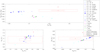 |
Fig. 1. Top panel: inferred fractional mass to ratio of radii for the α Cen system, obtained through various asteroseismic calibrations (see details in Tables 2 and 3). The calibrations are represented by different symbols (see legend). Cyan and blue symbols correspond to calibrations made with the Δν − ⟨δν0⟩ combination as seismic constraints: cyan for mass and effective temperature as non-seismic constraints, blue for fractional mass and radius ratio instead. Magenta, black, and green symbols respectively correspond to calibrations with r10, r02, and r13 used as seismic constraints. Open symbols indicates that no overshooting was included in the stellar models, while filled symbols denotes cases where models are computed with overshooting. The red cross and the dashed and dot-dashed lines respectively give the values inferred from the resolution of the orbital motion by K16 and K17, and the limits of the 1σ and 3σ error box on the K16 and K17 determinations. The red star indicates the parameters obtained from the P16 orbital solution. Bottom left panel: same as top panel, but for the inferred mass and radius of α Cen A. Bottom right panel: same as top panel, but for the inferred mass and radius of α Cen B. |
The first subset covers the calibrations in which the fractional mass and radius ratios were used as constraints. The names of the calibration include ‘Mfrac, Rratio’ and are depicted in blue. These models are the only ones to fall within or close to the 3σ error boxes on the fractional mass derived by K16. The radius ratio Γ is systematically lower than the K17 ratio: all these models clearly fail to reproduce this constraint. The three models with overshooting (and the only models in this subset with a convective core) and the model with a lower metallicity reproduce Γ with the lowest accuracy. Their position in a Hertzsprung-Russell diagram in the bottom panel of Fig. 2 confirms this tendency, as the four models differ by more than 1σ from the luminosities of α Cen A and α Cen B.
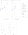 |
Fig. 2. Top left and right panels: large and small frequency separations of the final inferred models of α Cen A and B, for the various asteroseismic calibrations. Symbols are the same as those used in Fig. 1, except for the red cross and dashed line, which represent respectively the observed values and their 1σ error box, that we derived from the pulsation frequency analysis made by de Meulenaer et al. (2010). Bottom panels: Hertzsprung-Russell diagram for the results of the different calibrations compared to the observational values of K17. The A and B components are depicted respectively in the left and right panels. The legend details are the same as in the top panels. |
Results for α Cen A (in the bottom left panel of Fig. 1) indicate that only the lower metallicity model predicts a mass within 1σ to the mass of K16. The models with the GN93 mixture tend to masses higher than that of K16, and closer to that of P16. All the models but one predict a radius larger than K17, yet well within the 1σ limit on it.
Expected from the offset in the fitting of Γ, the radii predicted for α Cen B (bottom right panel of Fig. 1) by this subset of models present a systematic shift (but within 3σ) to the K17 value. The predicted masses are all within 1σ or 3σ of that of K16, except the model including surface effect correction. This model has a mass significantly lower than the K16 and P16 values. Again, the mass of the models calibrated with the GN93 mixture are the highest.
In Fig. 2 all the models of the B component (excepting the one with surface effect correction) reproduce within 1σ its large separation and are close to the lower 1σ limit for the small separation. As previously mentioned, this subset of models suggests higher masses and larger radii for the B component than the K16 values. The good fitting of the large separation (and thus the mean density) could either reveal a discrepancy between the seismic and astrometric plus interferometric solutions, or a degeneracy in the seismic solution. Given the difference between the observed TB, eff and especially LB (bottom right panel of Fig. 2) and those of the models, it is likely that we converged to a degenerate solution where the fitting of the large separation was privileged.
On the contrary, for the A component (top left panel of Fig. 2) the fit of the large separation systematically tends to larger values, hence overestimating its mean density. This same set of models reproduces the RA value from K16. Since they fit LA, the same is true for TA, eff, which is correlated to the determination of RA. Since MA predicted by the seismic models are higher than the K16 value, it likely reveals the origin of the mean density overestimation (which is confirmed by the inversions in Sect. 5). We note that due to the high precision on κ and Γ, we deal with a delicate trade-off in the adjustments of the seismic and non-seismic contributions in the χ2.
We also looked at the differences between observed and theoretical frequencies, which are shown in Fig. 3 for α Cen A. In the three panels we see for this subset of models that adopting the AGSS09 or GN93 mixture does not significantly change the accuracy of the frequency fitting. We note that for a model with overshooting (and the presence of a convective core) the differences with the observed frequencies are amplified.
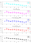 |
Fig. 3. Differences between the α Cen A observed frequencies and the theoretical frequencies from the models of the following calibrations (from top to bottom): A-Δνδν-R, Teff; A-Δνδν-Mfrac, Rratio; A-Δνδν-Mfrac, Rratio-GN93; A-Δνδν-Mfrac, Rratio-Ov; and A-r10-M, R. The different ℓ degrees of the modes shown are indicated in the insets. |
The second subset of solutions includes the three calibrations that are directly based on individual masses and effective temperatures (‘R, Teff’ in their names, depicted in cyan). They result in significantly lower κ values than in K16 and P16. They predict individual masses lower by ∼0.02 − 0.03 M⊙ than the K16 value for the B component, and close to the K16 value for the A component (see bottom panels in Fig. 1). This naturally results in decreasing the fractional mass κ in comparison to K16. Except for the calibration with the surface effect correction, the two other calibrations reproduce the individual radii of both components, and hence the radius ratio Γ. All three calibrations fit the Δν − ⟨δν0⟩ values for the B component within 1σ. They also fit the ⟨δν0⟩ of α Cen A (see Fig. 2). However, as in every other case, the fit of ΔνA results in larger values. For this smaller subset of models, LA is also poorly reproduced, which again raises the question of a discrepancy on the stellar constraints between seismic and non-seismic observables.
If we look at the quality of the fit based on the individual seismic frequencies in Fig. 3, we do not see any significant impact depending on the choice of the non-seismic constraints (see top two panels). More interestingly, we note a clear increasing trend with radial order in the differences between observed and theoretical frequencies, as in the Miglio & Montalbán (2005) and Eggenberger et al. (2004) studies. The amplitudes we get, of a few μHz, are of the same order as in the asteroseismic modelling by Miglio & Montalbán (2005, their Fig. 6) and lower than in Eggenberger et al. (2004).
The choice of the non-seismic constraints essentially impacts the masses and radii determinations of the system, as expected. Other inferred parameters do not show a parti-cular correlation depending of the choice of non-seismic observables. In particular, a similar range of ages is predicted by the two subsets, between ∼6.2 and ∼8.6 Gyr. This is in line with the ⟨δν0⟩ values (a marker of the evolution), which are similar for the two subsets.
4.1.2. GN93 vs AGSS09: Impact on the mass determination
We adopted the surface metallicity of Porto de Mello et al. (2008) as constraint for α Cen A and B in combination with the AGSS09 chemical mixture and OPAL opacities as input of the models in the majority of our calibrations. The means of the masses derived in these calibrations give ⟨MA⟩ = 1.098 ± 0.014 M⊙ and ⟨MB⟩ = 0.924 ± 0.011 M⊙. On the other hand, the means of the two calibrations adopting the GN93 mixture yield ⟨MA⟩ = 1.118 ± 0.017 M⊙ and ⟨MB⟩ = 0.945 ± 0.015 M⊙. The reason for the decrease in mass is likely to be related with a decrease in the opacity in the models with AGSS09. All things equal, for a given luminosity a metal-poor model will be less massive than a more metal-rich counterpart. However, because of degeneracies between the free parameters of the fitting, other elements, such as the initial composition, may generate differences in the output of calibrations with various physical ingredients. Hence we cannot exclude a combination of effects affecting the inferred masses when changing the chemical mixture.
For comparison with the literature, in their study Miglio & Montalbán (2005) did not observe a decrease in mass when switching from GN93 to the metallicity downward-revised Asplund et al. (2005) solar mixture. However, Miglio & Montalbán (2005) did only one study case based on these more metal-poor abundances (the A5 and B5 calibration in their Table 2), and employed a different seismic indicator. If we look at the results with the GN93 mixture, our values for ⟨MA⟩ and ⟨MB⟩ generally exceed by ∼0.015 M⊙ those derived by Miglio & Montalbán (2005). Other asteroseismic studies (e.g., Bazot et al. 2012; Nsamba et al. 2018) present methods and physics assumptions that diverge from ours, which hamper comparisons at a similar level of detail.
If we now look at the masses derived from the orbital solutions by K16 and P16, the update of the chemical mixture in the stellar models with AGSS09 predict a lower asteroseismic primary mass, but distant by less than its 1σ error from that of K16 (MA = 1.1055 ± 0.0039 M⊙). It is also lower than P16 (MA = 1.133 ± 0.005 M⊙), but distant by more than 2σ. For the secondary star, the asteroseismic mass (still considering AGSS09) is in agreement almost by 1σ with that of K16 (MB = 0.9373 ± 0.0033 M⊙), but is in disagreement with P16 (MB = 0.972 ± 0.005 M⊙). This asteroseismic determination is hence in overall agreement with the K16 solution, not with the P16 solution.
To understand the source of this disagreement, we first recall that the individual masses of K16 and P16 are obtained with help of the fractional mass of the system and a determination of the parallax. Since κ in K16 and P16 are so close, the differences between their estimation of the individual masses arise mainly from a difference in the parallax. If we compute κ with help of ⟨MA⟩ and ⟨MB⟩, we obtain ⟨κ⟩ = 0.457 ± 0.011, in good agreement with the orbital solutions of K16 and P16. So, two sources could explain our disagreement with the determination of P16. First, if we consider that our asteroseismic determination of the masses with AGSS09 are exact, it would indicate an error of accuracy on the parallax adopted in P16. To the contrary, if we consider the solution of P16 to be correct, it would question the role and adequacy of using the AGSS09 abundances for stellar models of α Cen AB stars (which are not exactly solar scaled, as shown in e.g., Morel 2018).
Considering the results with the more metal-rich GN93 mixture, the asteroseismic masses present values between the K16 and P16 solutions. For each component the determination with GN93 is closer to the K16 value (∼1σ) than to the P16 value (∼2σ).
4.1.3. OPAL vs OPLIB opacity
The role of the opacity in the stellar parameter inferences was explored in a calibration made with OPLIB data (Δνδν-Mfrac, Rratio-OPLIB). In comparison to its counterpart calibrations made with OPAL opacity (Δνδν-Mfrac, Rratio and Δνδν-Mfrac, Rratio-iniLM), the OPLIB calibration leads to a slight decrease in the masses of the system. This is expected since the OPLIB opacities are slightly lower than OPAL in the radiative regions of solar-type stars (Colgan et al. 2016).
4.1.4. Surface metallicity
The two calibrations where the surface metallicity of Bigot et al. (2008) is adopted lead to a less clear-cut result. Following the above reasoning on the opacity (see Sect. 4.1.2) we would expect to find lower masses than in the cases with the higher metallicity of Porto de Mello et al. (2008). However, the masses do not show such a systematic trend, and the calibrations with Bigot et al. (2008) predict similar ages to those with Porto de Mello et al. (2008). This actually indicates that the initial abundances adapt to compensate the effect of microscopic diffusion that will act on a similar timescale. The models calibrated with Bigot et al. (2008) thus present larger initial hydrogen abundances and lower initial metallicities, which result in a higher opacity in central region where free-free light absorption processes dominate. The larger X0 somehow mitigates the effect of a decrease in the metallicity and hence it barely affects the resulting masses.
4.1.5. Surface correction to frequencies
We included surface effect corrections, following Sonoi et al. (2015), in the Δνδν-R, Teff-Surf and Δνδν-Mfrac, Rratio-Surf cases. In the first calibration we see a decrease of ∼0.01 M⊙ and ∼800 Myr, although of the typical order of the error on ages, in the inferred stellar parameters by including surface correction. In the second case the masses of each component are the lowest we obtain in the whole set of calibrations. But we find it difficult in that case to reproduce the seismic indicators, which are the only ones out the 1σ box on Δν − ⟨δν0⟩ observed for each component (see large blue crosses in the top panels of Fig. 2). The surface metallicity is also poorly reproduced by this calibration. The corrections actually mostly deteriorate the ability to reproduce the Δν observed value by the two calibrations. The Sonoi et al. (2015) prescription tends to overcorrect even the low frequencies, while the surface effects are generally expected to be predominant at higher frequencies. The corrections could thus be overestimated for given frequencies and so introduce a bias in the Δν computed from the stellar models.
4.2. Calibrations based on r10, r02, r13
The calibrations based on frequency ratios (see Eq. (3)) are essentially sensitive to the central stellar conditions. They then suffer a lack of constraints on the global stellar parameters hindering convergence of the optimisation process. We adopted more stringent non-seismic constraints on the global stellar parameters, namely the K16 individual masses and the K17 radii and luminosities. As with the other set of seismic constraints, we also used the lowest oscillation frequency of each stellar component to improve the convergence to an acceptable seismic solution.
The Levenberg-Marquadt method converges, but results in inferences on the mass and radius for each star restricted to a similar narrow range of values, whatever ratios are used as seismic indicators; for instance, the results reproduce the RA values of K17 precisely, and the RB values within 1σ. As these models converge to heavier masses for the A component, and lighter masses for the B component, the κ they predict has thus an offset with the observed κ (see top panel of Fig. 1).
In Fig. 2, they all reproduce within 1σ the frequency small separations, as expected from their sensitivity to stratification in central stellar layers, which is also the case of the ⟨δν0⟩ indicator. However, all the results overestimate the large separation for the α Cen A, while they fit it with good accuracy for α Cen B. This could be expected from the bottom panel of Fig. 3 where the frequencies for a model of the A component calibrated with r10 show a larger departure from the observed frequencies than when using the ⟨δν0⟩ as a constraint.
All these calibrations predict ages between ∼5.55 and ∼6.35 Gyr, which are younger or at the lower limit of the range of ages predicted by the series of models from Sect. 4.1.1. The models obtained with the frequency ratios are an interesting test of the potential for inversions to discriminate age and whether the method can improve the accuracy on the ages determined with asteroseismology.
4.3. Age of the system and presence of a convective core
We show in Sect. 4.1.1 that the resulting models give a wide range of ages from ∼5.6 to ∼8.7 Gyr depending on the set of seismic constraints. Calibrations with frequency ratios as seismic indicators predict the youngest ages, ≲6.35 Gyr. Some of the α Cen A models that we obtained also present a convective core, but only in the cases where overshooting was included. We investigate the fitting accuracy of the models in more detail with help of r02 and r10, which are shown in Fig. 4. We compare four of the models with a convective core (A-Δνδν-Mfrac, Rratio-Ov and A-Δνδν-Mfrac, Rratio-Ov0.20, A-Δνδν-Mfrac, Rratio-GN93-Ov, A-r10-M, R-Ov) and a selection of models representative of the different resulting ages.
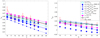 |
Fig. 4. Frequency ratios r02 (left panel) and r10 (right panel) for a selection of α Cen A models from the asteroseismic calibrations. The legend to both plots is given in the right panel. |
Looking at r02 in the left panel of Fig. 4, none of the selected models can reproduce all of the observed values. The model A-Δνδν-Mfrac, Rratio-Ov, with a convective core, is discarded by this indicator since it reproduces none of the observed values. The peak of r02 at n = 16 cannot be reproduced by any of the depicted models. Similarly, the observed dip of r02 at n = 23 is a feature that it hardly reproduced. Three of these models, including one with a convective core (A-Δνδν-Mfrac, Rratio-GN93-Ov), fit it, but then fail to fit the values at other n orders. Since none of the models shows such a dip and all of them are within 2σ of this value, the importance given to this signature has to be tempered. If we exclude this dip in the analysis, reproducing the overall behaviour of r02 tends to favour models without convective core, except the A-r10-M, R-Ov, which has one.
The internal structure profiles of all these models are shown in the left panel of Fig. 5. The models with a convective core have a marked inflection point in their sound speed (c) profile close to the centre because of the homogeneous chemical composition due to mixing by convection. Models without a convective core show a more or less sharp gradient of chemical composition depending on their state of evolution. This leads to a more pronounced contrast between the central and maximum (at normalised radius r/R ∼ 0.08) values of c. The sensitivity of r02 to stratification in those layers can thus deliver an indication on the age of the star. As seen in the left panel of Fig. 4, and referring to Table 4, models younger than ∼6.35 Gyr are indeed those that best reproduce this indicator, although a ∼7 Gyr model (A-Δνδν-R, Teff) is compatible at the margin. The three models that were clearly excluded (A-Δνδν-Mfrac, Rratio-GN93-Ov, A-Δνδν-Mfrac, Rratio-Ov, and A-Δνδν-Mfrac, Rratio-Surf) are also the oldest of the selection, respectively of 7.20, 8.12, and 8.66 Gyr.
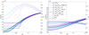 |
Fig. 5. Sound speed (thin lines) and hydrogen abundance (thick lines) for various calibration models of α Cen A (left panel) and B (right panel). The legend to both plots is given in the right panel. |
Focusing on the r10 indicator (right panel of Fig. 4), the model with the largest overshoot, αov = 0.2, is clearly disqualified. The other models with a convective core also seem to be excluded due to their inability to reproduce r10 for n = 18 to 23 (n = 21 to 23 for the A-r10-M, R-Ov model).
At n = 17, models with a convective core preferentially fit the observed dip, while only models without one can reproduce the peak observed at n = 21. However, as none of the models present these oscillating patterns in their r10 values, we must include with caution the importance given to these features in our analysis.
Considering the quality of the global fit of these indicators, it seems it favours the absence of a convective core in α Cen A. Nevertheless this conclusion is not definitive since the models without a convective core do not reproduce all of the features observed in r02 and r01.
Meanwhile, the three oldest models (7.20, 8.12, and 8.66 Gyr) should be discarded because of the r02 indicator. The models of 7.20 and 8.66 Gyr are also disqualified by the r10 indicator, while it is less clear for the 8.12 Gyr model. The r10 indicator also seems to discard the youngest model (5.55 Gyr; A-r10-M, R-Ov), while ruling it out from the fit of r02 is less clear. The most certain range that emerges is between ∼6.2 and ∼7 Gyr following the present analysis based on the frequency ratios.
This range is in good agreement with the asteroseismic calibrations of Eggenberger et al. (2004) and Miglio & Montalbán (2005), which derived models of between 5.5 and 7 Gyr in age. Our results also corroborate the recent determination by Morel (2018), which derives an age of ∼6 Gyr, based on the surface abundances of given chemical species.
α Cen B
The analysis of α Cen B with help of the frequency ratios is limited. Since we have a smaller number of frequencies observed for the secondary star, and with less precision, we have for instance only three measurements of r02 with larger error bars, as shown in Fig. 6.
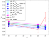 |
Fig. 6. Frequency ratios r02 for a selection of α Cen B models from the asteroseismic calibrations. |
As a consequence, r02 is difficult to use for retrieving information on the structure of the B component. For instance, the value of r02 at n = 20 is reproduced by all of the depicted α Cen B models in Fig. 6. None of the models is able to reproduce the observed value for the order n = 25 of r02, although this value looks like an outlier. We note an exception for n = 24. A look at Fig. 5 (right panel) of the central chemical composition (X) and sound speed (c) profiles of a selection of α Cen B models shows that models not reproducing r02 at this order are those with the highest values of X and c at the centre. It suggests that this is a possible way to estimate a threshold value of X or c at the centre. However, given the error on r02 and the non-reproduction of it at n = 25, it is impossible to firmly assert it.
5. Seismic inversions
The inversion results are presented in Fig. 7 for α Cen A and in Fig. 8 for α Cen B, illustrating the reference and inverted values for the mean density and SCore indicators for various reference models. We used multiple reference models fitted using different seismic constraints to take into account the model dependency of the inversion results. As can be seen from Fig. 7, this effect is the most significant contributor to the error budget.
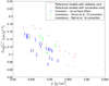 |
Fig. 7. Inversion results for α Cen A for both the mean density and the SCore indicator. Reference values from forward seismic modelling are given in red and orange, corresponding respectively to models without or with a convective core. Blue, green and black symbols represent the inversion results obtained with different treatments of surface effects (see legend). |
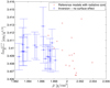 |
Fig. 8. Inversions results for α Cen B for both the mean density and the SCore indicator. Reference values from forward seismic modelling are given in red and inversion results in blue. |
The surface effect corrections of Ball & Gizon (2014) were also tested in addition to that of Sonoi et al. (2015), used to calibrate some reference models in the previous section. The Ball & Gizon (2014) correction was implemented directly in the SOLA cost function of the inversion, while the Sonoi et al. (2015) correction was implemented using their empirical law in log g and Teff. The surface effects, in particular those treated following Sonoi et al. (2015), have a significant but slightly less important impact than model dispersion. They actually do not increase the overall spread of the inversion results. Hence, for α Cen B, we only present inversion results without surface corrections as the total spread, which is the proper measure of the uncertainties, will be covered by the model-dependency effect.
From the inversion results, it appears that the SCore indicator is unable to firmly distinguish between the absence or presence of a convective core; there are indeed models both without or with a convective core in agreement with the inverted values. However, the inversion clearly rejects most of the models with ages older than 8 Gyr (the four reference models with the highest values of SCore in Fig. 7) previously found by the forward modelling approach. Similarly, the youngest model at ∼5.55 Gyr is also clearly discarded. It essentially favours models with ages between ∼5.9−7.3 Gyr, whilst an older model at 8.66 Gyr also appears compatible with SCore inverted values. The inversion also provides a 1% interval for the mean density values and it appears that half of the models are tilted outside of that interval.
It is actually possible to build models with or without a convective core agreeing with each other at the 1σ level for all individual frequencies. Such models will have extremely similar mean densities and frequency ratios, and thus cannot be distinguished by any seismic analysis technique. In these specific cases the inversion, which uses recombinations of the individual frequencies, cannot favour one of the two models.
Similar conclusions can be drawn for α Cen B since in this case the SCore inversion is not constraining. However, the mean density inversion provides similar constraints and shows that models are in slight disagreement with the inverted values. Overall, this implies that the inverted mean density values can be used to further constrain the models of both stars and especially their masses, but that the final decision on whether α Cen A harbours a convective core will most likely require more precise seismic data.
6. Conclusion
We reconsidered the seismic study of the α Cen AB binary, based on the oscillation frequency set of de Meulenaer et al. (2010) and the latest analyses of its orbital motion (P16, K16). In addition to a more traditional forward approach based on the large and small frequency separations, and frequency ratios, we also conducted asteroseismic inversions trying to answer the issue of the presence of a convective core in the primary component, α Cen A.
We first tested how different choices in the input physics of the models were affecting the results of the asteroseismic modelling. This is also a way to identify to what extent the current precision of the frequency dataset for α Cen AB can probe the stellar physics of models. Concerning the choice of the opacity data, we barely notice differences between the use of OPAL or OPLIB tables. The most influential element is the chemical mixture. We performed most of our seismic modelling using the determination of solar abundances by AGSS09; these models present lower metal abundances in comparison to previous determinations, such as GN93. For a given metallicity, a solar-like model will see its structure mainly altered by differences in the opacity because of reduced contributions from the metals. As a result, switching from GN93 models to AGSS09 models, we have observed a slight decrease in the masses deduced from asteroseismology of ∼0.02 M⊙ for both components.
We also compared these results with those of the orbital solutions by K16 and P16. The asteroseismic masses we obtained with GN93 fall between the K16 and P16 values, a bit closer to K16 than P16. The values obtained with AGSS09 are lower than those derived from the orbital solution by K16, but remain in agreement. They appear more in disagreement with the P16 orbital solution, however, in particular for the mass of the secondary component. We found one possible reason for this disagreement could be an error in accuracy on the parallax in P16. However, it also appeared worth questioning the adequacy of adopting solar-distributed abundances in stellar models of α Cen AB. With the determination of certain photospheric abundances made for this binary (e.g., Morel 2018), we could consider in the future building composition tables (and the associated opacity and equation of state tables) customised to the analysis of these two stars.
In parallel, we also focused on the age of the system, which we derived to be between 5.9 and 7.3 Gyr, regardless of the chemical composition adopted. This estimate is in good agreement with previous asteroseismic values of between 5.5 and 7 Gyr (e.g., Eggenberger et al. 2004; Miglio & Montalbán 2005). More recently, Morel (2018) estimated a similar age for the system, of ∼6 Gyr, based on an analysis of the photospheric abundances.
We finally looked at the presence of a convective core in α Cen A with help of the frequency ratios r02 and r10. Models with a convective core tend to be excluded by r10. This trend for excluding the presence of a convective core for models with AGSS09 differs from the conclusion of a recent study by Nsamba et al. (2019). On the contrary, these authors found seismic solutions with a convective core in most cases, whatever chemical mixture was selected.
We went a step further to resolve this challenging issue by attempting asteroseismic inversions of the mean density and an entropy indicator (see details on the method in Buldgen et al. 2015, 2018). The inversions converged for each of the inverted quantities, but the precision was insufficient to conclude firmly. While the inversions of the entropy indicator favour models without a convective core, some of the models with a convective core remain compatible with the inverted values. These first inversions are nevertheless encouraging; with a gain in precision on oscillation frequencies, inversions could leave no doubt. This gain would also be beneficial for α Cen B, on which we have attempted the same inversions; however, the results are presently inconclusive.
This new study shows how privileged and essential a system like α Cen AB is for studying the physics of solar-like stars. It demonstrates again the role of asteroseismology to determine fundamental stellar parameters and how it can highlight potential flaws in physical or observational data. The current precision on the oscillation frequency dataset for α Cen is now the main limiting factor for finer asteroseismic analysis. Achieving at least the same precision as that obtained on the 16 Cyg binary by the Kepler satellite appears a reasonable goal for such a bright system. However, its magnitude is paradoxically what hampers it for most observational facilities. New progress could be soon reached with the SONG project, and its extension to the south, a network of spectrographs specially designed for observing solar-like oscillations (e.g., Grundahl et al. 2009). Alternatively, the recent development of missions based on nanosatellites, a type with very moderate costs and reduced lifespan, offers an opportunity to solve this problem. The improvement of α Cen seismic data could indeed fit a dedicated nanosatellite project very well.
Due to the assumption of common formation, the parameters that α Cen B has in common with those of α Cen A are not repeated.
Acknowledgments
S.J.A.J.S. and P.E. have received funding from the European Research Council (ERC) under the European Unions Horizon 2020 research and innovation programme (grant agreement No 833925, project STAREX). V.V.G. is a F.R.S.-FNRS Research Associate. G.B. acknowledges fundings from the SNF AMBIZIONE grant No 185805 (Seismic inversions and modelling of transport processes in stars).
References
- Adelberger, E. G., García, A., Robertson, R. G. H., et al. 2011, Rev. Mod. Phys., 83, 195 [NASA ADS] [CrossRef] [Google Scholar]
- Angulo, C., Arnould, M., Rayet, M., et al. 1999, Nucl. Phys. A, 656, 3 [NASA ADS] [CrossRef] [Google Scholar]
- Asplund, M., Grevesse, N., & Sauval, A. J. 2005, in Cosmic Abundances as Records of Stellar Evolution and Nucleosynthesis, eds. T. G. Barnes, III, & F. N. Bash, ASP Conf. Ser., 336, 25 [Google Scholar]
- Asplund, M., Grevesse, N., Sauval, A. J., & Scott, P. 2009, ARA&A, 47, 481 [NASA ADS] [CrossRef] [Google Scholar]
- Baglin, A., Auvergne, M., Barge, P., et al. 2006, in The CoRoT Mission Pre-Launch Status – Stellar Seismology and Planet Finding, eds. M. Fridlund, A. Baglin, J. Lochard, & L. Conroy, ESA Spec. Publ., 1306, 33 [Google Scholar]
- Bahcall, J. N., Basu, S., Pinsonneault, M., & Serenelli, A. M. 2005, ApJ, 618, 1049 [NASA ADS] [CrossRef] [Google Scholar]
- Ball, W. H., & Gizon, L. 2014, A&A, 568, A123 [NASA ADS] [CrossRef] [EDP Sciences] [Google Scholar]
- Basu, S., & Antia, H. M. 2008, Phys. Rep., 457, 217 [NASA ADS] [CrossRef] [Google Scholar]
- Bazot, M., Bouchy, F., Kjeldsen, H., et al. 2007, A&A, 470, 295 [NASA ADS] [CrossRef] [EDP Sciences] [Google Scholar]
- Bazot, M., Bourguignon, S., & Christensen-Dalsgaard, J. 2012, MNRAS, 427, 1847 [NASA ADS] [CrossRef] [Google Scholar]
- Bazot, M., Christensen-Dalsgaard, J., Gizon, L., & Benomar, O. 2016, MNRAS, 460, 1254 [NASA ADS] [CrossRef] [Google Scholar]
- Bedding, T. R., & Kjeldsen, H. 2008, in 14th Cambridge Workshop on Cool Stars, Stellar Systems, and the Sun, ed. G. van Belle, ASP Conf. Ser., 384, 21 [Google Scholar]
- Bedding, T. R., Kjeldsen, H., Butler, R. P., et al. 2004, ApJ, 614, 380 [NASA ADS] [CrossRef] [Google Scholar]
- Bevington, P. R., & Robinson, D. K. 2003, Data Reduction and Error Analysis for the Physical Sciences (Boston, MA: McGraw-Hill) [Google Scholar]
- Bigot, L., Thévenin, F., & Kervella, P. 2008, Mem. Soc. Astron. It., 79, 670 [NASA ADS] [Google Scholar]
- Böhm-Vitense, E. 1958, ZAp, 46, 108 [NASA ADS] [Google Scholar]
- Borucki, W. J., Koch, D., Basri, G., et al. 2010, Science, 327, 977 [NASA ADS] [CrossRef] [PubMed] [Google Scholar]
- Bouchy, F., & Carrier, F. 2001, A&A, 374, L5 [NASA ADS] [CrossRef] [EDP Sciences] [Google Scholar]
- Bouchy, F., & Carrier, F. 2002, A&A, 390, 205 [NASA ADS] [CrossRef] [EDP Sciences] [Google Scholar]
- Buldgen, G., Reese, D. R., Dupret, M. A., & Samadi, R. 2015, A&A, 574, A42 [NASA ADS] [CrossRef] [EDP Sciences] [Google Scholar]
- Buldgen, G., Reese, D. R., & Dupret, M. A. 2016a, A&A, 585, A109 [NASA ADS] [CrossRef] [EDP Sciences] [Google Scholar]
- Buldgen, G., Salmon, S. J. A. J., Reese, D. R., & Dupret, M. A. 2016b, A&A, 596, A73 [NASA ADS] [CrossRef] [EDP Sciences] [Google Scholar]
- Buldgen, G., Reese, D. R., & Dupret, M. A. 2018, A&A, 609, A95 [NASA ADS] [CrossRef] [EDP Sciences] [Google Scholar]
- Buldgen, G., Salmon, S., & Noels, A. 2019, Front. Astron. Space Sci., 6, 42 [CrossRef] [Google Scholar]
- Butler, R. P., Bedding, T. R., Kjeldsen, H., et al. 2004, ApJ, 600, L75 [Google Scholar]
- Caffau, E., Ludwig, H.-G., Steffen, M., Freytag, B., & Bonifacio, P. 2011, Sol. Phys., 268, 255 [NASA ADS] [CrossRef] [Google Scholar]
- Carrier, F., & Bourban, G. 2003, A&A, 406, L23 [NASA ADS] [CrossRef] [EDP Sciences] [Google Scholar]
- Chaplin, W. J., & Miglio, A. 2013, ARA&A, 51, 353 [NASA ADS] [CrossRef] [Google Scholar]
- Colgan, J., Kilcrease, D. P., Magee, N. H., et al. 2016, ApJ, 817, 116 [NASA ADS] [CrossRef] [Google Scholar]
- Cox, J. P., & Giuli, R. T. 1968, Principles of Stellar Structure (New York: Gordon and Breach) [Google Scholar]
- de Meulenaer, P., Carrier, F., Miglio, A., et al. 2010, A&A, 523, A54 [NASA ADS] [CrossRef] [EDP Sciences] [Google Scholar]
- Demory, B.-O., Ehrenreich, D., Queloz, D., et al. 2015, MNRAS, 450, 2043 [NASA ADS] [CrossRef] [Google Scholar]
- Ducati, J. R. 2002, VizieR Online Data Catalog: II/237 [Google Scholar]
- Dumusque, X., Pepe, F., Lovis, C., et al. 2012, Nature, 491, 207 [NASA ADS] [CrossRef] [PubMed] [Google Scholar]
- Dziembowski, W. A., Pamyatnykh, A. A., & Sienkiewicz, R. 1990, MNRAS, 244, 542 [NASA ADS] [Google Scholar]
- Edmonds, P., Cram, L., Demarque, P., Guenther, D. B., & Pinsonneault, M. H. 1992, ApJ, 394, 313 [NASA ADS] [CrossRef] [Google Scholar]
- Edvardsson, B. 1988, A&A, 190, 148 [NASA ADS] [Google Scholar]
- Eggenberger, P., Charbonnel, C., Talon, S., et al. 2004, A&A, 417, 235 [NASA ADS] [CrossRef] [EDP Sciences] [Google Scholar]
- Ferguson, J. W., Alexander, D. R., Allard, F., et al. 2005, ApJ, 623, 585 [NASA ADS] [CrossRef] [Google Scholar]
- Fletcher, S. T., Chaplin, W. J., Elsworth, Y., Schou, J., & Buzasi, D. 2006, MNRAS, 371, 935 [NASA ADS] [CrossRef] [Google Scholar]
- French, V. A., & Powell, A. L. T. 1971, R. Greenwich Obs. Bull., 173, 63 [Google Scholar]
- Gough, D. 2003, Astrophys. Space Sci., 284, 165 [NASA ADS] [CrossRef] [Google Scholar]
- Grevesse, N., & Noels, A. 1993, in Origin and Evolution of the Elements, eds. N. Prantzos, E. Vangioni-Flam, & M. Casse, 15 [Google Scholar]
- Grevesse, N., & Sauval, A. J. 1998, Space Sci. Rev., 85, 161 [Google Scholar]
- Grundahl, F., Christensen-Dalsgaard, J., Arentoft, T., et al. 2009, Commun. Asteroseismol., 158, 345 [NASA ADS] [Google Scholar]
- Guenther, D. B., & Demarque, P. 2000, ApJ, 531, 503 [NASA ADS] [CrossRef] [Google Scholar]
- Hatzes, A. P. 2013, ApJ, 770, 133 [NASA ADS] [CrossRef] [Google Scholar]
- Iglesias, C. A., & Rogers, F. J. 1996, ApJ, 464, 943 [NASA ADS] [CrossRef] [Google Scholar]
- Irwin, A. W. 2012, Astrophysics Source Code Library [record ascl:1211.002] [Google Scholar]
- Joyce, M., & Chaboyer, B. 2018, ApJ, 864, 99 [NASA ADS] [CrossRef] [Google Scholar]
- Kaltenegger, L., & Haghighipour, N. 2013, ApJ, 777, 165 [NASA ADS] [CrossRef] [Google Scholar]
- Kamper, K. W., & Wesselink, A. J. 1978, AJ, 83, 1653 [NASA ADS] [CrossRef] [Google Scholar]
- Kervella, P., Thévenin, F., Ségransan, D., et al. 2003, A&A, 404, 1087 [NASA ADS] [CrossRef] [EDP Sciences] [Google Scholar]
- Kervella, P., Mignard, F., Mérand, A., & Thévenin, F. 2016, A&A, 594, A107 [NASA ADS] [CrossRef] [EDP Sciences] [Google Scholar]
- Kervella, P., Thévenin, F., & Lovis, C. 2017a, A&A, 598, L7 [NASA ADS] [CrossRef] [EDP Sciences] [Google Scholar]
- Kervella, P., Bigot, L., Gallenne, A., & Thévenin, F. 2017b, A&A, 597, A137 [NASA ADS] [CrossRef] [EDP Sciences] [Google Scholar]
- Kim, Y.-C. 1999, J. Korean Astron. Soc., 32, 119 [Google Scholar]
- Kjeldsen, H., Bedding, T. R., Frandsen, S., & Dall, T. H. 1999, MNRAS, 303, 579 [NASA ADS] [CrossRef] [Google Scholar]
- Kjeldsen, H., Bedding, T. R., Butler, R. P., et al. 2005, ApJ, 635, 1281 [NASA ADS] [CrossRef] [Google Scholar]
- Kjeldsen, H., Bedding, T. R., & Christensen-Dalsgaard, J. 2008, ApJ, 683, L175 [NASA ADS] [CrossRef] [Google Scholar]
- Lebreton, Y., & Goupil, M. J. 2014, A&A, 569, A21 [NASA ADS] [CrossRef] [EDP Sciences] [Google Scholar]
- Le Pennec, M., Turck-Chièze, S., Salmon, S., et al. 2015, ApJ, 813, L42 [NASA ADS] [CrossRef] [Google Scholar]
- Lund, M. N., Silva Aguirre, V., Davies, G. R., et al. 2017, ApJ, 835, 172 [CrossRef] [Google Scholar]
- Metcalfe, T. S., Chaplin, W. J., Appourchaux, T., et al. 2012, ApJ, 748, L10 [Google Scholar]
- Miglio, A., & Montalbán, J. 2005, A&A, 441, 615 [NASA ADS] [CrossRef] [EDP Sciences] [Google Scholar]
- Mondet, G., Blancard, C., Cossé, P., & Faussurier, G. 2015, ApJS, 220, 2 [NASA ADS] [CrossRef] [Google Scholar]
- Morel, T. 2018, A&A, 615, A172 [CrossRef] [EDP Sciences] [Google Scholar]
- Neuforge-Verheecke, C., & Magain, P. 1997, A&A, 328, 261 [NASA ADS] [Google Scholar]
- Neuforge, C., Pourbaix, D., Noels, A., & Scuflaire, R. 1999, in Upward Revision of the Individual Masses in A Cen: Implications for the Evolutionary State of the System, eds. J. B. Hearnshaw, & C. D. Scarfe, ASP Conf. Ser., 185, 335 [Google Scholar]
- Nsamba, B., Monteiro, M. J. P. F. G., Campante, T. L., Cunha, M. S., & Sousa, S. G. 2018, MNRAS, 479, L55 [Google Scholar]
- Nsamba, B., Campante, T. L., Monteiro, M. J. P. F. G., Cunha, M. S., & Sousa, S. G. 2019, Front. Astron. Space Sci., 6, 25 [CrossRef] [Google Scholar]
- Porto de Mello, G. F., Lyra, W., & Keller, G. R. 2008, A&A, 488, 653 [NASA ADS] [CrossRef] [EDP Sciences] [Google Scholar]
- Pourbaix, D. 1998, A&AS, 131, 377 [NASA ADS] [CrossRef] [EDP Sciences] [Google Scholar]
- Pourbaix, D., & Boffin, H. M. J. 2016, A&A, 586, A90 [NASA ADS] [CrossRef] [EDP Sciences] [Google Scholar]
- Pourbaix, D., Nidever, D., McCarthy, C., et al. 2002, A&A, 386, 280 [NASA ADS] [CrossRef] [EDP Sciences] [Google Scholar]
- Quarles, B., & Lissauer, J. J. 2016, AJ, 151, 111 [NASA ADS] [CrossRef] [Google Scholar]
- Rajpaul, V., Aigrain, S., & Roberts, S. 2016, MNRAS, 456, L6 [NASA ADS] [CrossRef] [Google Scholar]
- Reese, D. R., Marques, J. P., Goupil, M. J., Thompson, M. J., & Deheuvels, S. 2012, A&A, 539, A63 [NASA ADS] [CrossRef] [EDP Sciences] [Google Scholar]
- Roxburgh, I. W., & Vorontsov, S. V. 2003, A&A, 411, 215 [NASA ADS] [CrossRef] [EDP Sciences] [Google Scholar]
- Schou, J., & Buzasi, D. L. 2001, in SOHO 10/GONG 2000 Workshop: Helio- and Asteroseismology at the Dawn of the Millennium, eds. A. Wilson, & P. L. Pallé, ESA Spec. Publ., 464, 391 [Google Scholar]
- Scuflaire, R., Théado, S., Montalbán, J., et al. 2008a, Ap&SS, 316, 83 [Google Scholar]
- Scuflaire, R., Montalbán, J., Théado, S., et al. 2008b, Ap&SS, 316, 149 [Google Scholar]
- Silva Aguirre, V., Davies, G. R., Basu, S., et al. 2015, MNRAS, 452, 2127 [NASA ADS] [CrossRef] [Google Scholar]
- Sonoi, T., Samadi, R., Belkacem, K., et al. 2015, A&A, 583, A112 [NASA ADS] [CrossRef] [EDP Sciences] [Google Scholar]
- Tang, Y.-K., Bi, S.-L., Gai, N., & Xu, H.-Y. 2008, Chin. J. Astron. Astrophys., 8, 421 [NASA ADS] [CrossRef] [Google Scholar]
- Thévenin, F., Provost, J., Morel, P., et al. 2002, A&A, 392, L9 [NASA ADS] [CrossRef] [EDP Sciences] [Google Scholar]
- Thoul, A. A., Bahcall, J. N., & Loeb, A. 1994, ApJ, 421, 828 [NASA ADS] [CrossRef] [Google Scholar]
- Thoul, A., Scuflaire, R., Noels, A., et al. 2003, A&A, 402, 293 [NASA ADS] [CrossRef] [EDP Sciences] [Google Scholar]
- Wesselink, A. J. 1953, MNRAS, 113, 505 [NASA ADS] [CrossRef] [Google Scholar]
- Xu, Y., Takahashi, K., Goriely, S., et al. 2013, Nucl. Phys. A, 918, 61 [NASA ADS] [CrossRef] [Google Scholar]
- Yıldız, M. 2007, MNRAS, 374, 1264 [NASA ADS] [CrossRef] [Google Scholar]
- Yıldız, M. 2008, MNRAS, 388, 1143 [NASA ADS] [CrossRef] [Google Scholar]
All Tables
All Figures
|
Fig. 1. Top panel: inferred fractional mass to ratio of radii for the α Cen system, obtained through various asteroseismic calibrations (see details in Tables 2 and 3). The calibrations are represented by different symbols (see legend). Cyan and blue symbols correspond to calibrations made with the Δν − ⟨δν0⟩ combination as seismic constraints: cyan for mass and effective temperature as non-seismic constraints, blue for fractional mass and radius ratio instead. Magenta, black, and green symbols respectively correspond to calibrations with r10, r02, and r13 used as seismic constraints. Open symbols indicates that no overshooting was included in the stellar models, while filled symbols denotes cases where models are computed with overshooting. The red cross and the dashed and dot-dashed lines respectively give the values inferred from the resolution of the orbital motion by K16 and K17, and the limits of the 1σ and 3σ error box on the K16 and K17 determinations. The red star indicates the parameters obtained from the P16 orbital solution. Bottom left panel: same as top panel, but for the inferred mass and radius of α Cen A. Bottom right panel: same as top panel, but for the inferred mass and radius of α Cen B. |
| In the text | |
|
Fig. 2. Top left and right panels: large and small frequency separations of the final inferred models of α Cen A and B, for the various asteroseismic calibrations. Symbols are the same as those used in Fig. 1, except for the red cross and dashed line, which represent respectively the observed values and their 1σ error box, that we derived from the pulsation frequency analysis made by de Meulenaer et al. (2010). Bottom panels: Hertzsprung-Russell diagram for the results of the different calibrations compared to the observational values of K17. The A and B components are depicted respectively in the left and right panels. The legend details are the same as in the top panels. |
| In the text | |
|
Fig. 3. Differences between the α Cen A observed frequencies and the theoretical frequencies from the models of the following calibrations (from top to bottom): A-Δνδν-R, Teff; A-Δνδν-Mfrac, Rratio; A-Δνδν-Mfrac, Rratio-GN93; A-Δνδν-Mfrac, Rratio-Ov; and A-r10-M, R. The different ℓ degrees of the modes shown are indicated in the insets. |
| In the text | |
|
Fig. 4. Frequency ratios r02 (left panel) and r10 (right panel) for a selection of α Cen A models from the asteroseismic calibrations. The legend to both plots is given in the right panel. |
| In the text | |
|
Fig. 5. Sound speed (thin lines) and hydrogen abundance (thick lines) for various calibration models of α Cen A (left panel) and B (right panel). The legend to both plots is given in the right panel. |
| In the text | |
|
Fig. 6. Frequency ratios r02 for a selection of α Cen B models from the asteroseismic calibrations. |
| In the text | |
|
Fig. 7. Inversion results for α Cen A for both the mean density and the SCore indicator. Reference values from forward seismic modelling are given in red and orange, corresponding respectively to models without or with a convective core. Blue, green and black symbols represent the inversion results obtained with different treatments of surface effects (see legend). |
| In the text | |
|
Fig. 8. Inversions results for α Cen B for both the mean density and the SCore indicator. Reference values from forward seismic modelling are given in red and inversion results in blue. |
| In the text | |
Current usage metrics show cumulative count of Article Views (full-text article views including HTML views, PDF and ePub downloads, according to the available data) and Abstracts Views on Vision4Press platform.
Data correspond to usage on the plateform after 2015. The current usage metrics is available 48-96 hours after online publication and is updated daily on week days.
Initial download of the metrics may take a while.