| Issue |
A&A
Volume 645, January 2021
|
|
|---|---|---|
| Article Number | A65 | |
| Number of page(s) | 8 | |
| Section | Planets and planetary systems | |
| DOI | https://doi.org/10.1051/0004-6361/202039567 | |
| Published online | 13 January 2021 | |
Oligarchic growth in a fully interacting system
1
Konkoly Observatory, Research Centre for Astronomy and Earth Sciences, 1121,
Budapest,
Konkoly Thege Miklós út 15-17, Hungary
e-mail: This email address is being protected from spambots. You need JavaScript enabled to view it.
2
Department of Astronomy, Eötvös Loránd University, 1117
Budapest, Hungary
Received:
30
September
2020
Accepted:
11
December
2020
Abstract
Context. In the oligarchic growth model, protoplanets develop in the final stage of planet formation via collisions between planetesimals and planetary embryos. The majority of planetesimals are accreted by the embryos, while the remnant planetesimals acquire dynamically excited orbits. The efficiency of planet formation can be defined by the mass ratio between formed protoplanets and the initial mass of the embryo-planetesimal belt.
Aims. In numerical simulations of the oligarchic growth, the gravitational interactions between planetesimals are usually neglected due to computational difficulties. In this way, computations require fewer resources. We investigated the effect of this simplification by modeling the planet formation efficiency in a belt of embryos with self-interacting or non-self-interacting planetesimals.
Methods. We used our own graphics processing unit-based direct N-body integrator for the simulations. We compared 2D models using different initial embryo numbers, different initial planetesimal numbers, and different total initial belt masses. For a limited number of cases, we compared the 2D and 3D simulations.
Results. We found that planet formation efficiency is higher if the planetesimal self-interaction is taken into account in models that contain the commonly used 100 embryos. The observed effect can be explained by the damping of planetesimal eccentricities by their self-gravity. The final numbers of protoplanets are independent of planetesimal self-gravity, while the average mass of the formed protoplanets is larger in the self-interacting models. We also found that the non-self-interacting and self-interacting models qualitatively give the same results above 200 embryos. Our findings show that the higher the initial mass of the embryo-planetesimal belt, the higher the discrepancy between models that use self-interacting or non-self-interacting planetesimals is. The study of 3D models showed quantitatively the same results as the 2D models for low average inclination. We conclude that it is important to include planetesimal self-interaction in both 2D and 3D models in cases where the initial embryo number is less than 200.
Key words: planets and satellites: formation / celestial mechanics / methods: numerical
© ESO 2021
1 Introduction
The formation of terrestrial planets can last for 108 yr (see, e.g., Safronov 1972). The early phase of planetary assembly can be described as a runaway growth process in which the high mass bodies accrete more mass and grow rapidly due to gravitational focusing (Greenberg et al. 1978). The building blocks of planets are kilometer-sized planetesimals, which were formed from the dust component of the protoplanetary disk (Kokubo & Ida 2002). Runaway growth is followed by the next step of final assembly, oligarchic growth, in which the gravitational focusing is damped and the velocity dispersion between the neighboring bodies increases due to the perturbation of the larger bodies (Kokubo & Ida 1998). As a result, embryos that are massive enough to significantly perturb the planetesimals’ orbits are formed (Ida & Makino 1993). Subsequent collisions of embryos and planetesimals form the precursors of planets, called protoplanets (Rafikov 2003).
The mean iteration time (MIT) of a direct N-body simulation scales with the number of embryos (Ne, usually 100) and the number of planetesimals (Np, usually 1000) as  . However, the iteration time can be lowered to
 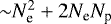 in a non-self-interacting model, where the planetesimals’ self-gravity is neglected or approximated.
Several studies have investigated the final assembly phase with direct N-body methods in a gas-free environment. Raymond et al. (2009) investigated the terrestrial planet formation in the inner Solar System after the dissipation of the nebular gas using the Mercury central processing unit-based (CPU-based) direct N-body code from Chambers (1999). In their model, there were 85–90 embryos (5 × 10⁻³−10−1 M⊕) and 1000–2000 planetesimals (2.5 × 10⁻³ M⊕) as well as a Jupiter and a Saturn mass giant. Embryo-embryo and embryo-planetesimal interactions were modeled, while planetesimal self-interaction was neglected due to calculation difficulties. Using a similar simplification for modeling terrestrial planet formation with the Mercury code, Ronco (2015) presented models that contain 45 embryos (6 × 10⁻²−4.7 × 10⁻¹ M⊕) and 1000 non-self-interacting planetesimals (2.68 × 10⁻³−2.1 × 10⁻² M⊕). In a recent study, Lykawka & Ito (2019) investigated the formation of the terrestrial planets in the Solar System using a modified version of the Mercury integrator (Hahn & Malhotra 2005; Kaib & Chambers 2016). Lykawka & Ito (2019) performed 540 simulations with 20–116 embryos and 2230–7000 non-self-interacting planetesimals.
Levison & Morbidelli (2007) investigated the formation of ice giants and the Kuiper belt using the SyMBA code (Levison & Duncan 2000). They ran models with three to six embryos (1 M⊕) and rings of 1000–32 700 planetesimals (10−2−8 × 10⁻² M⊕). In their models, planetesimal self-interaction was approximated by a radial force component based on the formalism from Binney & Tremaine (1987). Levison & Morbidelli (2007) found that neglecting self-gravity resulted in unphysical embryo motion because planetesimals were trapped in the 1:1 mean-motion resonance with embryos. This phenomenon is removed by approximating planetesimal self-gravity.
Quintana et al. (2007) investigated terrestrial planet formation in a binary star system. Their model contained a relatively low number of particles, 14 embryos (9.3 × 10⁻² M⊕), and 140 self-interacting planetesimals (9.3 × 10⁻³ M⊕), assuming a 50/50 embryo-to-planetesimal mass ratio. In another fully interacting model, Morishima, et al. (2008) simulated the formation of terrestrial planets. To model the very first phase (runaway growth), an approximation of the direct force calculation of 1000–5000 self-interacting planetesimals was applied (parallel tree code from Richardson et al. 2000). Fan & Batygin (2017) investigated the effect of planetesimal self-gravity on the evolution of the orbits of giant planets and Kuiper Belt objects. They used the QYMSYM graphics processing unit-based (GPU-based) N-body code (Moore & Quillen 2011) and compared self-interacting to non-self-interacting models, which contained 1000 planetesimals and the four giant planets. The orbital architecture of the final systems was similar; however, instabilities led to the destruction of the system in more cases with self-interacting models than with non-self-interacting ones.
In this study, we investigate how planetesimal self-interaction affects the planet formation efficiency (mass transfer efficiency between the initial bodies and the protoplanets) in the final assembly phase of planet formation. We use GPUs for the direct N-body calculations, which enables us to integrate fully interacting systems. We present models containing embryos embedded in the disks of self-interacting or non-self-interacting planetesimals. The effect of the initial embryo-to-planetesimal mass ratio is also investigated in both cases. Models with different embryo and planetesimal numbers are compared. This paper is organized as follows. In Sect. 2, we present the applied numerical integrator and the initial conditions. Section 3 contains the simulation results and a discussion. In Sect. 4, we summarize our main conclusions.
2 Numerical simulations
We modeled the oligarchic growth using N-body simulations. Initially, three types of bodies are presented in the system: a star, planetary embryos, and planetesimals. Thus, the simulated system does not contain gas. This model resembles the environment of the last phase of planet formation.
In this investigation, we compare two distinct models in which the systems contain: (i) gravitationally self-interacting planetesimals (hereafter INT) or (ii) non-self-interacting planetesimals (NON). The gravitational interaction between planetesimals is neglected, while the embryo-embryo, embryo-star, embryo-planetesimal, and star-planetesimal interactions are taken into account in NON models. In INT models, all bodies are in interaction with each other.
We used our own developed numerical integrator, HIPERION1, for the calculations; it is a GPU-based direct N-body integrator. We applied a fourth order Hermite scheme for all simulations (Makino & Aarseth 1992). The calculations were performed on NVidia Tesla K20 and K40 GPU cards. At each integration step, the optimal time-step is given by a fourth order version of the generalized Aarseth scheme (Press & Spergel 1988; Makino & Aarseth 1992). We verified the η parameter that controls the precision of the integrator in the range of 0.0025 ≤ η ≤ 0.04. We found the evolution of the total embryo mass to be independent of η. The precision of the integrator can be characterized by the relative energy error of the system, which is given by the ratio of the instantaneous energy to the initial system’s total (potential plus kinetic) energy (Nitadori & Makino 2008). By using a canonical setting η = 0.02, the relative energy error is found to be in the range of 10−6−10−3.
In our simulations, a close encounter of different bodies can result in the following phenomena: bodies collide and merge, bodies are engulfed by the star, or bodies are scattered out from the system. Only embryo-planetesimal or embryo-embryo collisions were allowed if the distance between the center of the two colliding bodies was smaller than their mutual radii. The collisions are assumed to be fully inelastic, that is, the total mass and momentum of colliding bodies are conserved. The total energy of the system is corrected by the energy loss that occurred during the collisions. The density of the bodies is assumed to be constant, and therefore the radius of the forming body is determined by the added mass. Thus, the fragmentation of the bodies is ignored, which has been proven to be a plausible approximation (Wetherill & Stewart 1993). Bodies are removed from the system if their distance to the star is less than 0.1 au or larger than 10 au.
The initial structure of the systems is the same in both the NON and INT simulations. The host star is represented by a 1 M⊙ central body. The inner boundary and the outer boundary of the simulated embryo-planetesimal belt are 0.4 and 4.2 au, respectively. The number density of embryos and planetesimals follows a power law of − 1 as a function of radial distance.
To investigate the statistical properties of the evolving systems first, we ran ten INT and ten NON models, each containing a belt of 100 embryos and 1000 planetesimals that were randomly distributed. The initial position of the embryos and planetesimals was redistributed ten times. The ten INT and the ten NON simulations were modeled in two dimensions, where the eccentricity and the inclination of the embryos, as well as those of the planetesimals, were set to zero. Additionally, we ran 3D models where the mean eccentricity and inclination of the embryos, as well as those of the planetesimals, were in the ranges of 10−5 −10−1 and 5 × 10⁻⁶−5 × 10⁻², respectively.
The total mass of the initial embryo-planetesimal belt is based on a scaled version of the Minimum Mass Solar Nebula (MMSN) model (Weidenschilling 1977; Hayashi 1981). The total mass of the embryo-planetesimal belt is 7.35 M⊕, which is three times greater than the dust mass of the solar nebula in this region and is a conservative calculation based on Lissauer (1987). The initial embryo-to-planetesimal mass ratio is 50/50. Embryos and planetesimals have uniform masses, and thus the individual initial masses of an embryo and a planetesimal are 4 × 10⁻² M⊕ and 4 × 10⁻³ M⊕, respectively. The radii of the embryos and planetesimals are calculated based on their masses and assuming a uniform 2 g cm−3 density, which gives 3000 and 1400 km in our standard models, respectively.
To understand the effect of planetesimal self-interaction, two INT and two NON models were applied, in which the initial embryo-to-planetesimal mass ratios were 25/75 and 75/25, respectively. The individual masses were corrected according to the mass ratios in these models.
To investigate the effect of the initial number of embryos and planetesimals, we performed two additional simulations: (i) four INT and four NON models consisting of 100 embryos and planetesimals in the range of 250–4000 and (ii) four INT and four NON models with embryo numbers in the range of 25–400 and 1000 planetesimals. The embryo-to-planetesimal mass ratio was fixed to 50/50.
3 Results and discussion
As a result of embryo–embryo and embryo–planetesimal collisions, the mass of embryos increases with time. The total mass confined by accreting embryos grows exponentially with time in the beginning. Later, the growth rate slows and the total embryo mass saturates. This phase determines the timescale of the simulations, which is found to be 2 × 10⁵ yr in all the 2D models and ~2 × 10⁶ yr in the 3D models, which is in agreement with the results of Kokubo & Ida (2000). The residual embryos can be considered protoplanets.
3.1 Properties of the final systems
First, we analyzed 10–10 2D models, where 100 embryos and 1000 planetesimals were initially in the system. In the INT models, nearly all the mass is converted to protoplanets. In the NON models, the number of the remnant planetesimals is significant at the end of simulations. As a result, the total mass of protoplanets is lower in the NON models than in the INT models, as can be seen in panel a ofFig. 1. The total protoplanetary mass (calculated for the 10–10 distinct models and represented by black lines in panel a of Fig. 1), is about 12 percent higher in the INT models than in the NON models.
Regarding the number of formed protoplanets, we found an average of 11.6 in the INT models and 13.1 in the NON models. The difference in the number of remnant planetesimals in the two models is significant: 18.5 in the INT models and 237.4 in the NON models. Namely, nearly 13 times more planetesimals are accreted by protoplanets in the INT models than in the NON models. As a consequence, the average masses of the protoplanets are 0.67 M⊕ and 0.53 M⊕ in the INT and NON models, respectively. The mean separations of the protoplanets’ orbits are 0.54 and 0.35 au, and the mean eccentricities of the protoplanets are 0.12 and 0.1, respectively.
We also investigated the effect of the initial embryo-to-planetesimal mass ratio (see the 25/75 and 75/25 mass ratios indicated with orange and green lines, respectively, in Fig. 1). We found that the difference between the INT and NON models regarding the total mass confined by protoplanets increases when the initial embryo mass decreases. We must emphasize that in the INT models the total mass that is transformed into protoplanets (~ 98%) does not depend on the initial embryo mass.
We will now discuss our findings regarding the efficiency of mass conversion to protoplanets. As a result of embryo-planetesimal interactions, the eccentricity of planetesimals is excited to high values and a population of highly eccentric planetesimals (HEPs) forms. We found that the cumulative number of planetesimals with a given eccentricity is constant up to a critical value and then drops steeply (see Fig. 2). The value of the critical eccentricity is found to be 0.1 for all models. Panel b of Fig. 1 shows the evolution of the number of HEPs. It is clear that the growth rate in the HEP number is much higher (resulting in a HEP number that is ten times higher) in the NON models compared to the INT models. Simulations that assume different embryo-to-planetesimal mass ratios show the same effect. The mean eccentricities of planetesimals are 0.09 and 0.44 at their maxima in the INT and NON models, respectively.
The difference in the total mass of the HEP population in the INT and NON models explains the difference in the total mass of protoplanets formed in the those models. In our simulations, HEPs are accreted with a lower probability, which explains the difference in the total mass of protoplanets in the INT and NON models.
In the oligarchic growth phase, the velocity dispersion as well as the eccentricity of the planetesimals increase due to the excitation of the embryos. Panel c of Fig. 1 shows the evolution of the root mean square (rms) eccentricity of the non-accreted planetesimal population for the ten standard INT models and the ten standard NON models, as well as the 25/75 and 75/25 mass ratio models. Panel c shows that the rms eccentricity increases with time, while the number of the remnant planetesimals decreases. As a result, the eccentricity of the relatively few non-accreted planetesimals is high. We note that HEPs will not be accreted by the embryos in the later phase.
One can also see in panel c of Fig. 1 that the rms eccentricity of the planetesimals grows more slowly in the INT models than in the NON models due to the self-gravity of planetesimals. On average, the rms eccentricity (which is not saturated) is about twice as much in the NON models than in the INT models. The start of the oligarchic growth phase is indicated by a purple horizontal line in panel c. It can be seen that all models are in the oligarchic growth phase for most of the integration time: The orderly growth phase lasts only for ~ 104 orbits, while the oligarchic phase lasts for ~7 × 10⁵ orbits at the inner edge of the embryo-planetesimal belt.
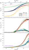 |
Fig. 1 Evolution of the embryo-planetesimal belt. Panela: evolution of the total mass confined by accreting embryos. The mass is normalized by the initial mass of the embryo-planetesimal belt. The top and bottom horizontal axes display the number of orbits at the inner and the outer edges of the belt, respectively. Dashed red lines and solid blue lines show the mass evolution of the 50/50 mass ratio in the NON and INT models, respectively. Black lines show the average for 10–10 models in both cases. Orange and green lines indicate models where a 25/75 and a 75/25 initial embryo-to-planetesimal mass ratio is assumed, respectively. Panelb: evolution of the number of the HEP population normalized with the total number of planetesimals in all models. Panelc: evolution of the planetesimal rms eccentricity. Above the horizontal purple line, the system is in the oligarchic growth phase. |
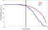 |
Fig. 2 Number of planetesimals (normalized with the initial number of planetesimals) that have an average eccentricity larger than a given eccentricity limit. The red and blue curves show the numbers of planetesimals in the NON and INT models, respectively (we note that the NON curve was divided by ten for the comparison with the INT curve). The vertical black line indicates the critical eccentricity value used to determine the HEP number. |
3.2 Effect of the initial embryo and planetesimal number
In the following, we investigate the effect of the number of bodies in the system. Panel a of Fig. 3 displays the evolution of the total embryo mass in models where the initial planetesimal number varies in the range of 250–4000 and the embryo number is the same (100) as in previous models. It can be seen that the total protoplanetary mass depends only weakly on the planetesimal number. Thus, the departure between the INT and NON models is independent of the initial planetesimal number. Regarding the number of HEPs, we found that the eccentricity evolution of planetesimals is also weakly dependent on the planetesimal number (see panel b of Fig. 3). We did not find any correlation between the number of initial and remnant planetesimals in either the NON or INT models. Based on the rms eccentricity evolution of planetesimals, NON models require only half the time to enter the oligarchic growth phase compared to INT models (see panel c of Fig. 3). This phenomenon is independent of the initial number of planetesimals.
Contrary to previous findings, the initial number of embryos affects the results in NON models (see Fig. 4). In NON models where the initial embryo number varies in the range of 25–400 and the planetesimal number is 1000, we observe a strong dependence of the total protoplanet mass on the initial embryo number: the larger the embryo number, the larger the mass transported to protoplanets. Thus, in NON simulations the planet formation efficiency increases with the initial embryo number. However, above a critical embryo number (found to be 200), the mass conversion is ~ 98 percent (see panel a of Fig. 4), which means that INT and NON models give the same results. One can see in panel b of Fig. 4 that the number of HEPs decreases with the increasing initial number of embryos and that above 200 practically no HEPs can be found. In these cases, the total mass of the formed protoplanets is equal in the INT and NON models. According to panel c of Fig. 4, the evolution of planetesimal rms eccentricity deviates between the NON and INT models. However, above 200 initial embryos, both models show the same rms eccentricity evolution for the majority of the simulation.
In the NON models, we find that the lower the initial number of embryos, the higher the planetesimal eccentricity is. We note that inour models the individual embryo mass is inversely proportional to the initial number of embryos because the embryo-planetesimal belt mass is kept fixed. Moreover, the high eccentricity excitation prevents the frequent accretion of the planetesimals in the assembly phase. As a result, the increasing embryo number leads to a weak excitation, and therefore the difference in the accretion efficiency of planetesimals between the INT and NON models decreases as well. Our results also show that the number of HEPs is very low in all INT models, independentof the initial number of embryos. This can be explained by the eccentricity damping effect of planetesimal self-gravity.
In the INT models, the results are independent of the initial embryo mass. This is due to the fact that planetesimal self-gravity strongly damps their eccentricity. Therefore, the individual embryo mass has no effect on the mass conversion to protoplanets.
The damping effect of planetesimal self-gravity is shown in Fig. 5, which displays the semimajor axis-eccentricity diagram of embryos and planetesimals in one INT model (panel a) and three NON models (panels b–d) at the same evolutionary phase. Comparing panels a and b, one can see that about 3/4 and 1/20 of planetesimals have been accreted in the INT and NON models, respectively. The mean eccentricities of non-accreted planetesimals are 0.19 and 0.34 in the INT and NON models, respectively. This is explained by the fact that the low-eccentricity planetesimals are accreted by the embryos with a higher probability compared to the HEPs.
To demonstrate the eccentricity excitation effect of the individual embryo mass, panels c and d of Fig. 5 show models with low and high initial embryo numbers, respectively. One can see that a large number of non-accreted planetesimals are in the system in the case of a low initial embryo number (high individual embryo mass; see panel c). Contrarily, for a high initial embryo number, practically no non-accreted planetesimals are present (see panel d). We emphasize that the INT model shows a similar conversion efficiency compared to a NON model with a high initial embryo number (see panels a and d).
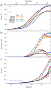 |
Fig. 3 Same as Fig. 1 but models use different initial numbers of planetesimals, and the number of embryos is fixed to 100. Colors represent models with different initial numbers of planetesimals in the rage of 250–4000. |
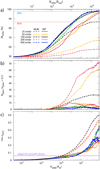 |
Fig. 4 Same as Fig. 1 but models use different initial numbers of embryos, and the number of planetesimals is fixed to 1000. Colors represent models with different initial numbers of embryos in the range of 25–400. |
3.3 Effect of the initial mass of embryo-planetesimal belts
The effect of the initial mass of embryo-planetesimal belts on the evolution of the total protoplanetary mass in INT and NON models was also investigated. We performed simulations with a 22.05 M⊕ initial mass belt, which is three times more massive than what was used in the models presented above. In these new models, initial embryo numbers ranging from 25 to 400, a constant 1000 planetesimals, and a 50/50 embryo-to-planetesimal mass ratio were used.
Figure 6 shows the evolution of the protoplanet mass in high-mass and standard-mass models. One can see that the departure between INT and NON models in the total protoplanetary mass is higher in the more massive belts compared to the less massive belts as long as fewer than 200 initial embryos are used. We also found that the INT and NON models show the same results for more than 200 initial embryos, regardless of the initial belt mass.
3.4 2D and 3D embryo-planetesimal belts
The time required to saturate the total protoplanetary mass strongly depends on the average orbital inclination of the interacting bodies: the higher the average inclination, the slower the saturation. This is because the probability of collisions is lower if the mutual inclination of embryos and planetesimals is higher. It should be noted that the simulations presented so far were calculated in 2D, where the orbits of interacting bodies are coplanar. To investigate the effect of planetesimal self-gravity in 3D, we also investigated five additional new models that start with dynamically excited embryo-planetesimal belts. The eccentricities and the inclinations follow the Rayleigh distribution (Lissauer 1993) and assume the 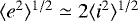 from Ida & Makino (1993). We investigated five different models where 10−5 ≤ σe ≤ 10−1 and 5 × 10⁻⁶ ≤ σi ≤ 5 × 10⁻², the initial mass ratio is 50/50, and the initial belt consists of 100 embryos and 1000 planetesimals.
Panel a of Fig. 7 shows the evolution of total mass confined by the accreting embryos in the 3D INT and NON models. For the initially moderately excited belts (σi ≤ 5 × 10⁻⁵), the total protoplanetary masses are saturated and show different conversion efficiencies in the INT and NON models (the same difference as in the 2D models, i.e., 12%). We note that the timescale of the embryo growth is about two times slower in the 3D models. The growth rate decreases by σi. Therefore, models with σi ≥ 5 × 10⁻⁴ are not saturated.
Panel b of Fig. 7 shows the evolution of the HEP number, which begins to grow at the 104th orbit in the σi ≤ 5 × 10⁻⁵ models, while it begins to grow at later times, the 105th orbit, at the inner edge of the embryo-planetesimal belt in the σi ≥ 5 × 10⁻⁴ models. We can also see that the number of HEPs is at least two times higher in highly excited models than the peak of the HEP number in the moderately excited models at the end of the simulations. The difference between the 3D INT and NON models can be explained by the same phenomenon that was identified in the 2D models: the eccentricity damping of self-gravity.
Panel c of Fig. 7 displays the evolution of the planetesimal rms eccentricity. One can see that the σ ≤ 5 × 10⁻⁵ models saturate at the ~4 × 10⁶th orbit (at theinner edge of the belt), while the highly excited models do not saturate in the investigated timescale. In moderately excited models, the oligarchic phase occurs about two times later compared to the 2D models. To enter the oligarchic growth phase, at least ten times more orbits are required for the initially highly excited models than for the moderately excited models (see panel c of Fig. 7). We also note that the rms eccentricity grows faster in moderately excited NON models than in INT models.
To summarize our findings, the higher the initial mean inclination of embryo and planetesimal orbits, the slower the growth rate of the embryos due to the lower probability of planetesimal accretion. However, we emphasize that neglecting planetesimal self-gravity has the same effect on the embryo growth in 3D as it does in 2D.
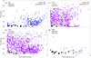 |
Fig. 5 Eccentricity of embryos and planetesimals as a function of the semimajor axis at the 3.1 × 10⁵th orbit at theinner edge. Panelsa and b: INT and a NON model, respectively, each initially with a 50/50 mass ratio, 100 embryos (black dots), and 4000 planetesimals (blue dots in the INT, purple dots in the NON model). Panelsc and d: NON models initially with 1000 planetesimals with 25 and 400 embryos, respectively. The size of black dots is proportionalto the one-third power of the embryo mass. |
 |
Fig. 6 Evolution of the total mass confined by the embryos in the INT and NON models. Red and blue shaded regions indicate the previously used embryo-planetesimal belt mass (7.35 M⊕) and the belt mass that is three times higher (22.05 M⊕), respectively. Colored curves represent models with different initial numbers of embryos (indicated in the key) in the range of 25–400 and with a constant 1000 planetesimals. |
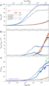 |
Fig. 7 Same as Fig. 1 but here 3D models are presented. Colors represent embryo-planetesimal disks with different initial mean eccentricities and inclinations in the INT and NON models, with an initial 100 embryos and 1000 planetesimals. The embryo-to-planetesimal mass ratio is 50/50. |
4 Conclusions
In this paper, we investigated the effect of planetesimals’ self-gravity on the final assembly phase of planet formation. In these models, the bodies of embryo and planetesimal populations are collided with each other to form growing embryos and, finally, protoplanets. Two types of models are compared: (i) self-interacting planetesimals (INT) and (ii) non-self-interacting planetesimals (NON). The circumstellar embryo-planetesimal belt consists of bodies with uniform masses. The total mass of the embryo-planetesimal belt is based on the MMSN model (Weidenschilling 1977; Hayashi 1981). We ran models with and without planetesimal self-gravity. We investigated the effect of both the initial number of planetesimals (250–4000) and embryos (25–400). The simulations ran for 2 × 10⁵ yr, which corresponds to 7.91 × 10⁵ and 2.32 × 10⁴ orbits at the inner and outer edges of the embryo-planetesimal belt, respectively. Beyond this time, only protoplanet collisions are observed and the planetesimal accretion is absent. We ran additional models with an embryo-planetesimal belt that was three times more massive, as well as with dynamically excited belts. We investigated the evolution of the planetesimal rms eccentricity. Based on our investigation, the modeled systems are predominantly in the oligarchic growth phase during the simulations. Our main results are the following.
- 1.
Simulations that started with a relatively large number of embryos (100) and planetesimals (1000) show that the total mass of the protoplanets is about 12% higher in the INT models than in the NON models. The number of remnant planetesimals (which are not accreted) is about an order of magnitude higher in NON simulations compared to INT simulations.
- 2.
Low-eccentricity planetesimals are easily accreted by the embryos, while the HEPs (e ≳ 0.1) remain in the system for a long time. Thus, the total protoplanetary mass at the end of the final assembly phase depends on the strength of the eccentricity excitation of planetesimals. The eccentricity excitation is highly damped in INT models, which results in a 98% efficiency in mass conversion from embryo and planetesimals to protoplanets. This can be explained by the effect of the eccentricity damping of planetesimal self-gravity.
- 3.
The total mass of the protoplanets is independent of the initial number of planetesimals (in the range of 250–4000) in both the INT and NON models that contain 100 embryos.
- 4.
In the simpler NON models, the total mass of protoplanets is proportional to the initial embryo number (with a constantplanetesimal number). However, above a critical embryo number (200), INT and NON models present the same results.
- 5.
The higher the initial mass of the embryo-planetesimal belt, the larger the discrepancy between the INT and NON models is, in terms of the final mass confined by protoplanets, assuming a commonly used initial embryo (≤100) and planetesimal (1000) number.
- 6.
The 3D simulations give qualitatively the same results as the 2D models. For 3D low average inclination models, we find a quantitative equivalence with the 2D results.
We emphasize that terrestrial planet formation is not complete at the end of our simulations. Protoplanets still perturbone another’s orbits and may collide with one another, leading to the formation of planets. Therefore, the architectural differences found in the INT and NON models (0.54 and 0.35 au mean separation; 0.67 and 0.53 M⊕ mean mass; 0.12 and 0.1 mean eccentricity of protoplanets) cannot be interpreted as appropriate orbital elements of the final planetary system. Terrestrial planet formation may cover a very long time, up to 108 yr, and we investigated a timescale that is shorter by three orders of magnitude. Thus, revealing the real architectural difference between theINT and NON models requires further study, where the protoplanetary systems are integrated further in time.
Here wemention some caveats of our models. First, we ignored the effect of fragmentation during collisions, which may affect the dynamics of the system and the embryo growth. However, according to Wetherill & Stewart (1993), fragmentation has no significant effect on embryo growth. Secondly, highly excited 3D models were not followed to protoplanetary mass saturation due to computational difficulties. However, based on our moderately excited models, we think that our findings can be generalized for 3D cases.
According to our simulations, the MIT increases linearly with the number of bodies in both the NON and INT models. We emphasize that the slope of the MIT-particle number curve is 1.23 times steeper in the INT models than in the NON models. However, the linearity breaks above 6000 bodies in the INT models due to the computational capability of the GPUs used for this investigation. Fortunately, our INT simulations are numerically convergent at a lower number of bodies (100 embryos and 1000 planetesimals) than this limit. As a result, our fully GPU-based direct N-body integrator is an efficient tool for investigating the final assembly of terrestrial planet formation.
We emphasize that the evolution of the protoplanet mass does not depend on the accuracy of the integrator (the relative energy error is found to be in the range of 10−6−10−3), but rather on the initial number of bodies. We have shown that the initial number of bodies in the N-body models with non-self-interacting planetesimals may have a significant effect on the efficiency of mass transfer from small bodies to protoplanets. We conclude that numerical simulations of the final assembly phase of terrestrial planet formation require a relatively large number of embryos (≳ 200) if the planetesimal self-interactions are neglected. However, N-body simulations that are not simplified by neglecting planetesimal-planetesimal interactions are numerically convergent with a lower number of embryos. Thus, if the applied hardware for the numerical solution is highly sensitive to the number of particles (e.g., a CPU-based direct integrator), we suggest using at least twice as many fully interacting embryos than conventionally applied.
Acknowledgements
We thank the anonymous referee for useful suggestions that helped to improve the quality of the paper. This work was supported by the Hungarian Grant K119993. We acknowledge the Hungarian National Information Infrastructure Development Program (NIIF) for awarding us access to the computational resource based in Hungary at Debrecen.
References
- Binney, J., & Tremaine, S. 1987, Galactic Dynamics (Princeton, NJ: Princeton University Press) [Google Scholar]
- Chambers, J. E. 1999, MNRAS, 304, 793 [NASA ADS] [CrossRef] [MathSciNet] [Google Scholar]
- Fan, S., & Batygin, K. 2017, ApJ, 851, L37 [CrossRef] [Google Scholar]
- Greenberg, R., Wacker, J. F., Hartmann, W. K., & Chapman, C. R. 1978, Icarus, 35, 1 [NASA ADS] [CrossRef] [Google Scholar]
- Hahn, J. M., & Malhotra, R. 2005, AJ, 130, 2392 [NASA ADS] [CrossRef] [Google Scholar]
- Hayashi, C. 1981, Prog. Theor. Phys. Suppl., 70, 35 [NASA ADS] [CrossRef] [MathSciNet] [Google Scholar]
- Ida, S., & Makino, J. 1993, Icarus, 106, 210 [NASA ADS] [CrossRef] [MathSciNet] [Google Scholar]
- Kaib, N. A., & Chambers, J. E., 2016, MNRAS, 455, 3561 [NASA ADS] [CrossRef] [Google Scholar]
- Kokubo, E., & Ida, S. 1998, Icarus, 131, 171 [Google Scholar]
- Kokubo, E., & Ida, S. 2000, Icarus, 143, 15 [Google Scholar]
- Kokubo, E., & Ida, S. 2002, ApJ, 581, 666 [Google Scholar]
- Levison, H. F., & Duncan, M. J. 2000, AJ, 120, 2117 [NASA ADS] [CrossRef] [Google Scholar]
- Levison, H. F., & Morbidelli, A. 2007, Icarus, 189, 196 [NASA ADS] [CrossRef] [Google Scholar]
- Lissauer, J. J. 1987, Icarus, 69, 249 [NASA ADS] [CrossRef] [Google Scholar]
- Lissauer, J. J. 1993, ARA&A, 31, 129 [NASA ADS] [CrossRef] [Google Scholar]
- Lykawka, P. S., & Ito, T. 2019, ApJ, 883, 130 [CrossRef] [Google Scholar]
- Makino, J., & Aarseth, S. J. 1992, PASJ, 44, 141 [NASA ADS] [Google Scholar]
- Moore, A., & Quillen, A. C. 2011, New Astron., 16, 445 [CrossRef] [Google Scholar]
- Morishima, R., Schmidt, M. W., Stadel, J., & Moore, B. 2008, ApJ, 685, 1247 [NASA ADS] [CrossRef] [Google Scholar]
- Nitadori, K., & Makino, J. 2008, New Astron., 13, 498 [NASA ADS] [CrossRef] [Google Scholar]
- Press, W. H., & Spergel, D. N. 1988, ApJ, 325, 715 [NASA ADS] [CrossRef] [Google Scholar]
- Quintana, E. V., Adams, F. C., Lissauer, J. J., & Chambers, J. E. 2007, ApJ, 660, 807 [NASA ADS] [CrossRef] [Google Scholar]
- Rafikov, R. R. 2003, AJ, 125, 942 [NASA ADS] [CrossRef] [Google Scholar]
- Raymond, S. N., O’Brien, D. P., Morbidelli, A., & Kaib, N. A. 2009, Icarus, 203, 644 [NASA ADS] [CrossRef] [Google Scholar]
- Richardson, D. C., Quinn, T., Stadel J., & Lake, G. 2000, Icarus, 143, 45 [NASA ADS] [CrossRef] [Google Scholar]
- Ronco, M. P., de Elía, G. C., & Guilera, O. M. 2015, A&A, 584, A47 [NASA ADS] [CrossRef] [EDP Sciences] [Google Scholar]
- Safronov, V. S. 1972, Evolution of the Protoplanetary Cloud and Formation of the Earth and Planets (Jerusalem: Keter Publishing House) [Google Scholar]
- Weidenschilling, S. J. 1977, Ap&SS, 51, 153 [Google Scholar]
- Wetherill, G. W., & Stewart, G. R. 1993, Icarus, 106, 190 [NASA ADS] [CrossRef] [PubMed] [Google Scholar]
All Figures
|
Fig. 1 Evolution of the embryo-planetesimal belt. Panela: evolution of the total mass confined by accreting embryos. The mass is normalized by the initial mass of the embryo-planetesimal belt. The top and bottom horizontal axes display the number of orbits at the inner and the outer edges of the belt, respectively. Dashed red lines and solid blue lines show the mass evolution of the 50/50 mass ratio in the NON and INT models, respectively. Black lines show the average for 10–10 models in both cases. Orange and green lines indicate models where a 25/75 and a 75/25 initial embryo-to-planetesimal mass ratio is assumed, respectively. Panelb: evolution of the number of the HEP population normalized with the total number of planetesimals in all models. Panelc: evolution of the planetesimal rms eccentricity. Above the horizontal purple line, the system is in the oligarchic growth phase. |
| In the text | |
|
Fig. 2 Number of planetesimals (normalized with the initial number of planetesimals) that have an average eccentricity larger than a given eccentricity limit. The red and blue curves show the numbers of planetesimals in the NON and INT models, respectively (we note that the NON curve was divided by ten for the comparison with the INT curve). The vertical black line indicates the critical eccentricity value used to determine the HEP number. |
| In the text | |
|
Fig. 3 Same as Fig. 1 but models use different initial numbers of planetesimals, and the number of embryos is fixed to 100. Colors represent models with different initial numbers of planetesimals in the rage of 250–4000. |
| In the text | |
|
Fig. 4 Same as Fig. 1 but models use different initial numbers of embryos, and the number of planetesimals is fixed to 1000. Colors represent models with different initial numbers of embryos in the range of 25–400. |
| In the text | |
|
Fig. 5 Eccentricity of embryos and planetesimals as a function of the semimajor axis at the 3.1 × 10⁵th orbit at theinner edge. Panelsa and b: INT and a NON model, respectively, each initially with a 50/50 mass ratio, 100 embryos (black dots), and 4000 planetesimals (blue dots in the INT, purple dots in the NON model). Panelsc and d: NON models initially with 1000 planetesimals with 25 and 400 embryos, respectively. The size of black dots is proportionalto the one-third power of the embryo mass. |
| In the text | |
|
Fig. 6 Evolution of the total mass confined by the embryos in the INT and NON models. Red and blue shaded regions indicate the previously used embryo-planetesimal belt mass (7.35 M⊕) and the belt mass that is three times higher (22.05 M⊕), respectively. Colored curves represent models with different initial numbers of embryos (indicated in the key) in the range of 25–400 and with a constant 1000 planetesimals. |
| In the text | |
|
Fig. 7 Same as Fig. 1 but here 3D models are presented. Colors represent embryo-planetesimal disks with different initial mean eccentricities and inclinations in the INT and NON models, with an initial 100 embryos and 1000 planetesimals. The embryo-to-planetesimal mass ratio is 50/50. |
| In the text | |
Current usage metrics show cumulative count of Article Views (full-text article views including HTML views, PDF and ePub downloads, according to the available data) and Abstracts Views on Vision4Press platform.
Data correspond to usage on the plateform after 2015. The current usage metrics is available 48-96 hours after online publication and is updated daily on week days.
Initial download of the metrics may take a while.