| Issue |
A&A
Volume 645, January 2021
|
|
|---|---|---|
| Article Number | A35 | |
| Number of page(s) | 18 | |
| Section | Numerical methods and codes | |
| DOI | https://doi.org/10.1051/0004-6361/202038973 | |
| Published online | 05 January 2021 | |
SP_Ace v1.4 and the new GCOG library for deriving stellar parameters and elemental abundances⋆
INAF-Osservatorio Astronomico di Padova, Vicolo dell’Osservatorio 5, 35122 Padova, Italy
e-mail: This email address is being protected from spambots. You need JavaScript enabled to view it.
Received:
20
July
2020
Accepted:
1
October
2020
Abstract
Context. Ongoing and future massive spectroscopic surveys will collect very large numbers (106–107) of stellar spectra that need to be analyzed. Highly automated software is needed to derive stellar parameters and chemical abundances from these spectra.
Aims. We present the new version of SP_Ace (Stellar Parameters And Chemical abundances Estimator) a code that derives stellar parameters and elemental abundance from stellar spectra. The new version covers a larger spectral resolution interval (R = 2000−40 000) and its new library covers bluer wavelengths (4800–6860 Å).
Methods. SP_Ace relies on the General-Curve-Of-Growth (GCOG) library based on 6700 absorption lines whose oscillator strengths were calibrated astrophysically. We developed the calibration method and applied it to all the lines. From the new line list obtained we build the GCOG library, adopting an improved method to correct for the opacity of the neighboring lines. We implemented a new line profile for the code SP_Ace that better reproduces that of synthetic spectra. This new version of SP_Ace and the GCOG library has been tested on synthetic and real spectra to establish the accuracy and precision of the derived stellar parameters.
Results. SP_Ace can derive the stellar parameters Teff, log g, [M/H], and chemical abundances with satisfactory results; the accuracy depends on the spectral features that determine the quality, such as spectral resolution, signal-to-noise ratio, and wavelength coverage. Systematic errors were identified and quantified where possible. The source code is publicly available.
Key words: methods: data analysis / atomic data / stars: fundamental parameters / stars: abundances / techniques: spectroscopic / surveys
SP_Ace version 1.4 is available on the German Astrophysical Virtual Observatory web server at the address http://dc.g-vo.org/SP_ACE.
© ESO 2021
1. Introduction
The Gaia data releases (Gaia Collaboration 2018) have opened new avenues and have changed our approach and perspectives on the formation of the Milky Way. The potential for new discoveries has been further amplified by the addition of chemical information from ongoing spectroscopic surveys such as the Sloan Extension for Galactic Understanding and Exploration (SEGUE; Beers et al. 2006); the RAdial Velocity Experiment (RAVE; Steinmetz et al. 2006); the Large Sky Area Multi-Object Fiber Spectroscopic Telescope (LAMOST; Newberg et al. 2012); the Apache Point Observatory Galactic Evolution Experiment (APOGEE; Majewski 2012); the Gaia-ESO Public Spectroscopic Survey (Gilmore et al. 2012); the GALactic Archaeology with HERMES (GALAH) survey (Freeman et al. 2012).
However, the new findings are generally based on limited sets of chemical abundances. Moving forward, the upcoming massive spectroscopic surveys such as WEAVE (Dalton et al. 2014); the Sloan Digital Sky Survey (SDSS-V; Kollmeier et al. 2017); the Dark Energy Spectroscopic Instrument (DESI; DESI Collaboration 2016); the 4-Metre multi-Object Spectroscopic Telescope (4-MOST; de Jong et al. 2019); and the Multi-Object Optical and Near-infrared Spectrograph (MOONS; Cirasuolo et al. 2014), which are targeting millions of stars and exploring all the components of the Milky Way, hold a tremendous potential.
In particular, the William Herschel Telescope Enhanced Area Velocity Explorer (WEAVE) is the next step among the large Galactic spectroscopic survey that will be active in the near future. The WEAVE very large field of view (two-degree diameter), high multiplexing capability (∼1000 fibers), good resolution (R = 5000 and 20 000), and wide spectral coverage (3660–9500 Å) makes it uniquely equipped to conduct surveys for Galactic Archaeology. WEAVE will provide measurements based on low-resolution spectra of radial velocities, effective temperature, surface gravity, and metallicity for targets in the faint part of the Gaia catalogs with magnitudes in the range 16 < G < 20.7, which are too faint for the Gaia spectroscopy. In addition, its spectral range in the high-resolution mode allow us to measure transitions for about 17 species, probing the main nucleosynthetic channels (light elements, α, Fe peak, s- and r-process neutron-capture elements) for the vast majority of the stars in the magnitude range 12 < G < 16. WEAVE is currently in the phase of final survey definition, survey planning, and preparation of the first year of observations and will be at the telescope by the end of 2020 or early 2021. Several Galactic archaeology sub-surveys are already planned, including low- and intermediate-latitude disks, high-latitude halos, open and globular clusters, targeting about 3–4 million stars in the field and in open clusters (Jin et al., in prep.).
This tremendous amount of data poses formidable analysis and modeling challenges. Highly automated software is needed to derive stellar parameters and chemical abundances for these stars. WEAVE stellar spectra will be analyzed by a pipeline based on FERRE (Aguado et al. 2017) which will, however, derive the stellar parameters log g, Teff, [M/H], and a handful of chemical elements. More detailed analysis, including the derivation of the abundances of key chemical species required by specific scientific cases call for additional software.
The Stellar Parameters And Chemical abundances Estimator code SP_Ace (Boeche & Grebel 2016, hereafter Paper I) is one of those software packages. This code was already successfully used in a number of papers to analyze RAVE and LAMOST data (see, e.g., Boeche et al. 2011, 2018; Valentini et al. 2017). In this paper we present an updated version of the code with improved data treatment. Although the revision of the code was decided for the analysis of WEAVE stellar spectra (in particular for FGK high- and intermediate-metallicity stars), the present released version is for general purposes, suitable to be used on spectra with spectral resolutions in the range R = 2000−40 000 and wavelength range covering the interval 4800–6860 Å. The SP_Ace version specifically designed for WEAVE (v1.4W) will be presented in a future paper.
The paper is organized as follows: in Sect. 2 we briefly outline the basis of SP_Ace; in Sect. 3 we discuss the line list selection, including the calibration and the validation of the log gf values; in Sect. 4 we describe the construction of the equivalent width (EW) library and the final General-Curve-Of-Growth (GCOG) library; in Sect. 5 we present the main improvements in the code; in Sect. 6 we deal with the validation of the code using both synthetic and real stellar spectra. Finally the main conclusions are drawn in Sect. 7.
2. The code SP_Ace
SP_Ace is a FORTRAN90/95 code that derives stellar parameters (such as effective temperature Teff, gravity log g, and metallicity [M/H]) and elemental abundances from stellar spectra. Here we briefly recall the basics of SP_Ace; we refer the reader to Paper I for more details.
SP_Ace belongs to the class of codes that estimate the stellar parameters through spectral fitting, i.e., searching for the best match between the observed spectrum and a spectrum model. While other methods usually get their spectrum model from the many offered by libraries of synthetic spectra, SP_Ace constructs the spectrum model on the fly retrieving information of the central wavelengths and strengths of the spectral lines from the GCOG library specifically prepared for SP_Ace and, by assuming a line profile, produces a spectrum model from this information. SP_Ace calculates many spectrum models with different Teff, log g, [M/H], and elemental abundances [El/H] of several elements looking for the best match with the observed spectrum using a χ2 minimization routine.
The use of a GCOG library gives SP_Ace the flexibility to be directly applied to spectra of any spectral dispersion and resolution1. The GCOG library does not hold information such as spectral dispersion, spectral resolution, and radial velocity. These parameters are inferred by SP_Ace during the spectrum analysis; therefore, SP_Ace can analyze spectra with different spectral resolutions2, different spectral dispersions (which can be non-constants), and a range of radial velocities3, with no need to change or tweak the GCOG library or the measured spectra. Full details of GCOG library and how it was realized are given in Paper I, although in Sect. 4 of this paper we outline its basic concepts.
Before putting together a GCOG library, we have to take some necessary steps. To build the GCOG of a spectral line we need to know its EW value as a function of the stellar parameters, which implies the knowledge of its atomic parameters. Thus, we have to start from the creation of a line list that includes robust atomic and molecular parameters.
3. The line list
SP_Ace was designed for full spectral fitting. This implies the use of wide wavelength intervals on which all the absorption lines bring their contribution to the χ2 analysis. In order to have a realistic strength of these lines, we need a full line list with robust atomic parameters. As already discussed in Paper I, a large fraction of the line atomic parameters available in atomic databases, such as the Vienna Atomic Line Database (VALD; Kupka et al. 1999) or the NIST Atomic Spectra Database (Kramida et al. 2013), yield somewhat unreliable line strengths due to the inaccuracy of the oscillator strengths (f, often expressed as a logarithm log gf, where g is the statistical weight).
Under this condition we opted to perform an astrophysical calibration of the atomic parameters in order to fix and/or remove the lines with the larger errors. In what follows we describe how we chose and calibrated the line list.
3.1. Initial line list selection
We selected the initial line list from the VALD database (Kupka et al. 1999). We retrieved all the absorption lines with wavelength between 4800 and 6860 Å that have a central depth larger than 1% of the normalized continuum in any of the synthetic spectra of the Sun, Arcturus, and Procyon4. Combining the three line lists, we obtained an initial list of 14 025 lines belonging to atoms and a few molecules.
Whenever needed, we added to the line list atomic lines from Kurucz hyperfine line list (Kurucz 1995) and atomic and molecular lines from the luke.lst line list provided with the spectral synthesis software SPECTRUM (Gray & Corbally 1994) that was built from several sources, as reported in the SPECTRUM user manual. In some cases we chose to add some “dummy” lines that, although not present in any of the line sources in use, were able to account for the lines observed in real spectra. These dummy lines are further discussed in Sects. 3.3 and 3.5.
3.2. Spectra selection
To calibrate the atomic parameters of the selected line list, in this work we apply the same basic concepts outlined in Paper I, which we briefly summarize here. For this purpose we used the observed spectra of five standard stars: the Sun and Arcturus (spectra from Hinkle et al. 2000), Procyon, ϵ Eri, and ϵ Vir (from Blanco-Cuaresma et al. 2014, with the features reported in Sect. 4.1 of Paper I). All these spectra were provided already normalized by the authors; we just cited and used them “as is” (but re-normalized them later during the calibration process, see Sect. 3.3). We synthesized the spectra of these five standard stars, and compared the match of the synthetic lines to the observed ones. Then, the log gf values were changed to produce the best simultaneous fit of the five observed spectra.
The synthesis of the spectra was done with the software SPECTRUM (Gray & Corbally 1994), unlike in Paper I where we used MOOG (Sneden 1973) instead. While for normal (i.e., not broad) lines the two programs appear to perform similarly, we preferred SPECTRUM thanks to its more accurate synthesis of strong lines such as the H-α and H-β Balmer lines present in the wavelength window considered. These lines, together with the Na I doublet at 5889 and 5895 Å, are hard-coded into the SPECTRUM software, and therefore the calibration process is not applied to these four lines. In addition to the log gf calibration, we also calibrated the van der Waals (VdW) broadening parameter for some (but not all) lines (see Sect. 3.3 for details).
We used the stellar atmosphere models from the ATLAS9 grid (Castelli & Kurucz 2003) updated to the 2012 version5 linearly interpolated to the stellar parameters of the standard stars.
The stellar parameters adopted for the synthesis, such as Teff, log g, [M/H], micro-turbulence ξ, and macro-turbulence vmac, are listed in Table 1. The stellar parameters adopted for Arcturus were taken from Ramírez & Allende Prieto (2011), except for metallicity. To account for the alpha-enhancement of Arcturus, we applied the Salaris formula (Salaris et al. 1993)
![Mathematical equation: $$ \begin{aligned} \mathrm [M/H] = [Fe/H] + \log _{10}(0.638\cdot 10^{[\alpha /Fe]}+0.362) \end{aligned} $$](/articles/aa/full_html/2021/01/aa38973-20/aa38973-20-eq1.gif) (1)
(1)
and α/Fe = 0.27, which is the average of the relative abundances [El/Fe] of the elements Mg, Si, Ca, and Ti reported by Ramírez & Allende Prieto. The parameters of Procyon, ϵ Eri, and ϵ Vir are taken from Jofré et al. (2014).
Effective temperature (K), gravity, metallicity (dex), micro- and macro-turbulence (in km s−1) adopted to synthesize the spectra of the standard stars.
The values in Tables 1 and 2 differ from the corresponding values in Tables 1 and 2 of Paper I. These values were set by hand after eye inspection of the goodness of match between the observed and synthetic spectra, as described in Sects. 4.1 and 4.3 of Paper I. The macro-turbulence was applied to the synthetic spectra by using the utility software “macturb”, while the spectral resolution was matched by smoothing the synthetic spectra by applying the full width at half maximum (FWHM) with the utility “smooth2” provided with SPECTRUM. The spectral dispersion adopted is 0.01 pix Å−1.
Instrumental FWHMs adopted for the synthetic spectra in the four wavelength ranges.
The next step is to set the elemental abundances of the standard stars. For the Sun, we assume that all the abundances are zero ([El/H] = 0) adopting the solar abundances of Grevesse & Sauval (1998). For the other standard stars, we do not know the abundances of all the elements. However, during the calibration process the abundances can be adjusted as explained in Sect. 3.4, which is also a method used to derive them in an independent way6. We just need to set the initial abundances as starting point. As initial elemental abundances we used the available values provided by Jofré et al. (2015) for the elements Mg, Si, Ca, Sc, Ti, V, Cr, Mn, Co, Fe, and Ni. For any other element the initial abundance is set equal to the metallicity [El/H] = [M/H].
3.3. log gf calibration: method and software
To automatize the log gf calibration we wrote a software in Python3 with a graphical interface that is more user-friendly. As in Paper I, we divide the calibration into two steps that are repeated iteratively until convergence: the log gf calibration and the abundance calibration. The first step can be done interactively (thanks to the graphical interface) or in batch mode. The second is done by manually changing the abundances of the synthesized standard spectra. The procedure is similar to the one reported in Paper I.
For the calibration procedure, we use a working line list based on lines retrieved from the VALD database (described in Sect. 3.1). The working line list can be pruned of or enriched with lines taken from two auxiliary line lists: the SPECTRUM line list and the Kurucz hyperfine line list. The calibration is done iteratively on a calibrating interval 1.2 Å wide, and it moves from smaller to larger wavelengths. The log gf values of the lines inside the 1.2 Å are calibrated by using a minimization routine. In addition to these lines, the software also uploads the neighboring lines, ±5 Å on either side. These extra lines are not used for calibration, but for the re-normalization of the observed spectrum (the re-normalization routine is described in detail in Sect. 7.4 of Paper I). Although the standard spectra are already normalized, the normalizations commonly applied (such as the IRAF continuum) are prone to continuum underestimation in regions that are crowded by lines (see discussion in Sect. 7.4 of Paper I.). Our re-normalization based on the best matching spectrum avoids this underestimation and homogenizes the way the standard spectra are normalized7.
The minimization routine employs the trust-region reflective least-squares algorithm to find the best match between synthetic and observed spectra by changing iteratively the log gf of every line in the calibrating interval, synthesizing the standard spectra and evaluating the total χ2 at every change8. The optimization of log gf is limited to the values between −12 and +3. Beyond these limits the lines are rejected.
To speed up the calibration process, we first run the software in batch mode to calibrate the whole working line list and then we checked by eye every angstrom of the wavelength window, adding or removing lines when, in our judgment, it was necessary to improve the match. After any manual change the calibration of the whole calibrating interval was re-run in batch mode.
In some cases the working line list and the two auxiliary line lists were not enough to identify all the observed absorption lines. In the effort to identify unidentified lines, we developed a method (described in Appendix A) based on a simple machine learning (ML) model such as the k-nearest neighbors algorithm (from the Python scikit-learn package, Pedregosa et al. 2011) that permits the user to guess the excitation potential, log gf, and the element the line belongs to. This method seems to render good results, although it must still be considered experimental.
We employed this method in a few cases (146 lines out of 6700) in order to cover those lines for which there was no other possibility of explanation with the currently available line lists. The guessed lines allowed in our line list show a good match between the synthetic and the observed spectra for all the five standard stars.
Several strong lines have wide wings that the synthesis cannot properly reproduce with the standard broadening parameters. The software SPECTRUM allows the user to adjust the VdW broadening of the line through a fudge parameter. For our calibrating software we created a window dedicated to the setting of this fudge factor from where the user can calibrate it to match the wings of the observed line. Similarly to the log gf calibration, the calibration of the VdW parameter is performed by using a routine that minimizes the χ2 by changing the fudge factor. We performed the VdW parameter calibration for several lines (409 out of 6700), mostly belonging to Fe. This calibration does not run in batch mode and it was performed interactively.
3.4. Elemental abundances setting
After the first log gf calibration we look at the elemental abundances adopted for the standard stars used and consider whether these need to be reset. For this purpose the software measures and stores other useful quantities. Among the most important quantities are NEWR and purity. We define the normalized equivalent width residual (NEWR) for the ith line and the kth star as
where Fi is the flux integrated over an interval centered on the ith line. The superscript synt and obs refer to the synthetic or observed spectrum, respectively. The integration interval chosen is the width of the line at half of its maximum. This value (different from the one used in Paper I) estimates the lack or the excess of absorbed synthetic flux with respect to the quantity needed to match the observed flux, expressed in terms of log gf (or abundance).
On the other hand, the quantity purity expresses how much of the absorbed flux observed over a given absorption line is due to that line. We defined the purity as follows. Consider a synthetic line l with central wavelength w surrounded by some neighbor lines which may be blended with the line l. Let σ be the width of the spectral line and Fall the absorbed flux integrated over an interval 2σ wide centered on l on a synthetic spectrum where the line l and all its neighboring lines are present. Let Fall − 1 be the same integrated flux when all the neighboring lines but the line l are present. We compute
With this definition, purity is equal to one when the line is isolated. Otherwise, the closer to zero it is, the less the line contributes to the flux absorbed over the integration interval. From the just given definitions we infer that the smaller the purity, the less precise the quantity NEWR, because the integrated absorbed flux is more affected by the neighboring lines. Nonetheless, the quantity NEWR is important to evaluate the goodness of the match in the wavelength region over each absorption line and used to evaluate the consistency of the elemental abundances adopted.
In Fig. 1 we compare the NEWRs values of two elements before and after the log gf calibration and elemental abundances adjustment only for lines with purity > 0.9. In the left panels of Fig. 1 (i.e., before the calibration) we see a large dispersion of the NEWRs shifts of their average with respect to zero. The abundances are adjusted by hand, and then the log gf calibration is repeated. This process is iteratively performed by the user in order to make the averages and dispersions of the NEWRs distributions as close to zero as possible. The iteration is repeated until no more improvement is seen.
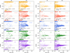 |
Fig. 1. Distributions of the NEWRs of the elements Si and Fe as a function of their EW for the five standard stars before (left) and after (right) the calibration. The standard stars are indicated by different colors (from top to bottom): the Sun (yellow), Arcturus (red), Procyon (blue), ϵ Vi (green), and ϵ Eri (purple). The triangles represent lines for which NEWR is larger than +0.4 or smaller than −0.4. In each panel the mean and the Pearson correlation parameter r are shown. |
In Table 3 we report the final abundances reached as a result of our log gf calibration. Some of these elements (O, Pr, and Sm) are considered not robust and are rejected (see discussion in Sect. 6.2.1).
Final chemical abundances for the five stars derived as result of the log gf calibration.
In addition to the abundance adjustment, we used the plot in Fig. 1 to adjust the micro-turbulence, which affects the shape of the distribution by creating different slopes between the low and the high EW regions. This is explained in Sect. 4.3 of Paper I, whereas an example of the different slopes taken by the NEWR distributions is shown in Fig. 5 of the same paper. Our final micro-turbulences are reported in Table 1.
3.5. Final line list
The log gf calibration was iterated after any adjustment of the abundances, and the iteration stopped when no more improvements were seen. During this procedure we checked by eye every angstrom of the interval to evaluate the goodness of the match between synthetic and observed spectra and, when needed, added or removed the necessary lines. All the lines that were involved in this process were stored in a file. The file contains a total of 14 514 absorption lines, some of which are flagged as valid and calibrated, some others as rejected lines. Not all of them were used to build the final GCOG library since the weaker lines were neglected and, as we explain in Sect. 4.1, the final line list contains 6700 lines.
We would now like to say few words about guessed lines and lines belonging to hyperfine splitting bands. In some cases we decided to use the “guess line” option (see Appendix A) to guess an unidentified absorption line, and in some cases these lines were used in the final line list used to build the GCOG library. Although there is some probability that these lines may be mismatched, we believe that the overall error in parameters and abundances may be smaller by keeping these lines than by leaving the unidentified line unfit. Similar considerations can be made for the lines belonging to the hyperfine splitting bands. To fit these bands we used the lines found in the auxiliary line list by Kurucz. However, by using these lines the software was not always able to find a good fit during the calibration. In these cases we took the liberty of removing some lines of the band that were not necessary to match the band shape, or manually added dummy lines (with the same atomic parameters of the hyperfine splitting band but a manually adjusted wavelength) in order to match the observed band shape. In this case we were not interested in using the right number of lines that compose a band (or the exact wavelength), but in reproducing the shape and the absorbed flux of it because this is what matters during estimation of stellar parameters and abundances.
3.6. Validation of log gf
In order to evaluate the reliability of our results, in Fig. 2 we compare our calibrated log gf values to the values reported in two literature works. In the left panel we show the comparison against the original log gf values provided by the VALD database: the statistic of the residuals (calibrated minus comparison values) shows no significant offset, but a standard deviation of 0.36. As discussed in Sect. 3, this is expected because of the inaccuracy of many theoretical log gf values. To better constrain our accuracy, in the middle panel we compare our calibrated log gf values to those obtained from the NIST database, limiting the comparison to the NIST lines that report an error in the gf value that is smaller than 10%. This selection leaves us with 527 lines belonging to several elements that show an offset of −0.08 and a standard deviation of 0.18. This is an offset close to the value found in Paper I (−0.125, see Fig. 6 of the same paper and its discussion in Sect. 4.6).
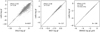 |
Fig. 2. Comparison between the calibrated log gf values (y-axis) and those of three different databases. Left: comparison with the VALD values for calibrated lines used for the final GCOG library. Center: comparison with the NIST values that have an estimated accuracy lower than 10% of the gf-value. Right: comparison with the BRASS values obtained with the grid method for Fe lines only. The statistics were computed on the residuals calibrated minus original log gf after a 3σ clipping. |
The Belgian Repository of fundamental Atomic data and Stellar Spectra (BRASS; Laverick et al. 2019) provides a good opportunity to compare the results of our calibration procedure with a similar one. In this work Laverick and colleagues evaluated the quality of the literature oscillator strengths with astrophysical values derived with two methods. The first, called the curve-of-growth (COG) method, requires the computation of the COG of the absorption line, and the log gf is derived as a function of the EW of the line. The second method, called the grid method, requires the synthesis of the line, and the log gf is derived from the best match of the synthetic line with the observed one. In both methods this is performed on seven standard stars, and the log gf values derived on these stars are then averaged to obtain the optimal log gf values from the COG method and from the grid method. For our purposes we chose to compare our calibrated log gf values to those that, in the Laverick work, have the robust-to-systematic flag (i.e., no blending issues) and the quality assessment flag (the COG and grid methods have overlapping error bars). However, for a fair comparison, the abundance zero point has to be set. Because of the different solar abundances adopted, to bring the values to a common zero point to the Laverick et al. values we added the difference between the solar abundances by Grevesse & Sauval (1998) (adopted by us) and those by Grevesse et al. (2007) (adopted by Laverick et al.). The comparison for Fe lines only is shown in the right panel of Fig. 2, using as reference the log gf values derived with the grid method. The offset is negligible and the standard deviation is as small as 0.06. The two results are in good agreement.
3.7. Accuracy of calibrated log gf
During the log gf calibration procedure we checked by eye the match between synthetic and observed spectra for every angstrom of their wavelength extension. However, this may not be enough to guarantee the accuracy of every line’s log gf because there are several sources of uncertainties. Some lines have non-LTE effects that our LTE synthesis cannot reproduce. The same applies to the 3D effects neglected by the plane-parallel atmosphere models we adopted. Particularly crowded blends of lines cannot be fully resolved. Uncertainties in the continuum placement of just 0.5% can heavily affect the apparent strength of a weak line the software is trying to match. Looking at trusted stellar parameters, we chose our standard stars among the best known we could find in the literature. However, they come from different sources and their parameters are derived with different methods that are also affected by errors.
All the error sources we cited (and others we did not cite here, see also Sect. 4.6 of Paper I) can drive errors in unpredictable directions which are difficult, if not impossible to track. The idea to use simultaneously many standard spectra to calibrate the log gf values is an attempt to frame all the error sources through statistics. If the Teff of a chosen standard spectrum is overestimated, another one may be underestimated. If one absorption line is weak in a standard hot dwarf star, it can be strong in a giant star where the calibrating software can match the line with a synthetic one with smaller errors. Therefore, the use of many standard stars during the log gf calibration averages out the individual systematic errors that we may find in the individual stars’ stellar parameters, continuum placement, and elemental abundances adopted. Thus, an improvement in our work can be made by raising the number of standard stars employed, with stellar parameters covering the largest parameter interval possible.
To summarize the underlying errors, we can compare our results with precise log gf values from laboratory measurements or with the results of similar works, as we did in Sect. 3.6. With log gf derived as we did, we are confident that SP_Ace is subject to the smallest possible systematic errors.
4. The GCOG library
As briefly explained in Sect. 2, in the GCOG library we store the coefficients of the polynomial functions that return the EWs of the absorption lines as a function of the stellar parameters Teff, log g, [M/H], and abundance [El/M] (one polynomial function per line). In order to derive these coefficients we need to compute the EWs across the parameter space and then compute the coefficients by fitting the EWs with a polynomial function.
4.1. The EW library
For the first step, i.e., building the EW library, we use the calibrated line list described in Sect. 3, pruned of the weak absorption lines, meaning those lines that contribute less than 3% of the normalized flux in all five standard spectra. After the pruning, the line list comprises 6700 lines. For each of these lines, we compute the EWs on a grid of points that uniformly covers the stellar parameter space. The grids of the four stellar parameters are as follows:
– The Teff grid covers the interval [3600, 7400] K with steps of 200 K;
– The log g grid covers the interval [0.2, 5.4] with steps of 0.4;
– The [M/H] grid covers the interval [−2.4, +0.4] dex with steps of 0.2 dex;
– The [El/M] grid covers the interval [−0.4, +0.6] dex with steps of 0.2 dex.
This translates into 3900 points that cover essentially the entire parameter space spanned by FGK-type stars. To compute the EWs we synthesized (by using SPECTRUM) every line for each of the grid points and integrated their absorbed flux. The micro-turbulence adopted for each grid point is derived by a function of the variables Teff and log g, as described in Appendix A of Paper I.
After computing the EWs, the library is not ready yet. The EWs just computed are obtained by synthesizing the lines as they were isolated. This is not always true; for blended lines the EWs need to be corrected for the opacity of the neighboring lines. An exhaustive discussion about why we need this correction can be found in Sect. 5.1 of Paper I. However, here we outline the main idea for a better understanding of the next section.
SP_Ace builds its spectrum model by summing up line profiles with EWs provided by its library and then subtracts the result from a normalized continuum. For an isolated line, the EW previously computed is the correct one, which allows SP_Ace to closely reproduce the corresponding synthetic line. However, this is not always true when the line belongs to a blend feature. As discussed by Sennhauser et al. (2009), when the lines composing the blend are optically thin (i.e., weak lines), a good approximation of the blend can be obtained by summing up the lines. On the other hand, when the lines are optically thick, their sum can easily produce a total depth that is larger than one and the total EW of the blend so constructed is larger than the one obtained with a synthesis. Therefore, to use SP_Ace we need to correct the EWs of the lines (by weakening them) that are blended with optically thick lines so that, by summing them up, the total EW of the blend will be close to the correct value that we would get with a synthesis. In the next section we show how to perform such a correction.
4.2. Correction for the opacity of the neighbors lines
With respect to Paper I, in this work we adopt a different opacity correction that allows us to reproduce lines blends more precisely. In this paper we make use of Eq. (20) by Sennhauser et al. (2009) that provides the correct depth of a blend features composed by two lines. The equation is
where Rtot represents the total depth of the blend composed of two lines that, if isolated, would have depths R1 and R2. In the case of blends composed of n lines, we apply this formula iteratively as
 (2)
(2)
where Ri is the total depth of the blend when the ith line has been summed up, while Ri − 1 is the total depth of the blend when the i − 1th line has been summed up.
Now we can outline the algorithm we used to compute the corrected EWs. Consider a blend composed of n lines. Then, the following operations are performed:
1. Synthesize the whole blend and compute its EW by integrating the total absorbed flux. We call this  ;
;
2. Order the lines by decreasing low excitation potential Ep, so that ith and i + 1th lines have Epi > Epi + 1;
3. synthesize each of the lines as if it were isolated over a common wavelength range that covers the whole blend. The normalized flux is  , while
  is the continuum;
4. Given that the depth of the lines is R = 1 − F, apply Eq. (2) iteratively for all the lines following the given order to obtain the partial depths of the blend  when the ith line is considered. The value
  is the depth of the full blend when all the lines have been considered;
5. Compute the depth that the ith line has in the blend as
6. Compute the corrected EW for the ith line by integrating the absorbed flux as
In particular, the total EW of the full blend so constructed is computed as
7. Compute the final corrected EW of the ith line by first normalizing the value  to the value
  as
as
Some explanation is needed to clarify the second and the last steps. The second step is applied to simulate the way that the absorption through the stellar atmosphere takes place. Assuming blackbody radiation moving through the several layers that compose the stellar atmosphere model from bottom up, a given wavelength λ is absorbed by all the absorbers (lines) that compose the considered blend in order of decreasing excitation potential. This is because the higher the excitation potential of the absorber, the deeper in the atmosphere the absorption takes place. This is only an approximation of what really happens because the absorption does not happen in a precisely confined atmosphere depth but over an interval of it, so that the intervals of different absorbers can overlap. However, the approximation adopted is helpful for SP_Ace to compute more realistic absorbed fluxes.
The last step is implemented because Eq. (2) provides an approximation that degrades with larger optical thickness. While this approximation is good for most of the lines, we saw that it does not work well in cores of very close and strong lines, leading to  . To fix this, we transform the value
  by keeping the proportion
  .
.
4.3. The GCOG library
With the corrected EWs seen in the previous section we can compute the GCOG library that is used by SP_Ace to build the spectrum models. The EW library now contains the EWs of every line for the 3900 grid points that cover the full stellar parameter space considered. In other words, these 3900 EWs map the GCOG of the line. In principle we could model the full parameter space with a polynomial function of the parameters Teff, log g, [M/H], and [El/M]. In practice, to avoid using a too high degree polynomial (which would require a high number of coefficients), we decided to use a fourth-degree polynomial over smaller regions centered over each parameter grid point. As reported in Sect. 6.1 of Paper I, this smaller region extends over 800 K in Teff, 1.6 in log g, 0.8 dex in [M/H], and 1.0 dex in [El/M]. Thus, we used a least-squares minimization routine to find the coefficients of a fourth-degree polynomial that fit best the 750 EWs that cover the smaller region surrounding every grid point. In this way SP_Ace can move through the parameter space and retrieve EWs from the GCOG library. The EWs, being continuous functions, smoothly and continuously change without discontinuities. To assess the reliability of the polynomial GCOGs in reproducing the correct EWs, in Fig. 3 we plot the residuals between the polynomial EWs and the ones stored in the EW library. For convenience, in Fig. 3 the y-axis expresses the residuals as abundances dex as
where EWpoly is the EW from the polynomial GCOG function and EWlib is the one from the EW library. The residuals are mostly smaller than 0.05 dex, confirming the reliability of the polynomial GCOGs.
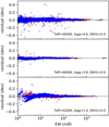 |
Fig. 3. Residual between the EWs in the EW library and that obtained from the GCOG library, expressed in abundance dex for lines with EW > 1 mÅ for three different atmosphere parameters. Red crosses, gray points, and blue triangles represent the EWs for the abundances [El/M] = +0.2, 0.0, and −0.2 dex, respectively. |
5. SP_Ace version 1.4
With respect to Paper I, where SP_Ace was released in its version 1.0, the code has undergone some revisions reported in the user manual provided with the code. In this work we present version 1.4.
The main changes concern the line profile. As in the previous version, we use the Voigt line profile by McLean et al. (1994), which is a function of the parameters γG and γL that rule the widths of the Gaussian and the Lorentzian parts, respectively. With the new SP_Ace version, the γL parameter is a polynomial function of the variables EW, γG, log g, and Teff. Details about this new function that expresses γL are given in Appendix B. We summarize here the main changes and new features coming with the new SP_Ace version 1.4:
– Improved line profile which is a function of the variables EW, γG, log g, and Teff;
– Extended capability to process spectra with size up to 128 000 pixels;
– Number of measured abundance up to 21 elements;
– Extended capability to measure spectra up to spectral resolution R = 40 000;
– New wavelength coverage 4800−6860 Å;
– Freedom to choose the input parameter file name, which allows the user to launch multiple processes (for parallel computing) in the same directory.
In addition, we fixed some bugs and optimized some routines to improve speed performance.
6. Validation
To establish the precision and accuracy of the SP_Ace measurements, we performed tests on synthetic and real spectra, comparing the SP_Ace results with the expected ones. The tests were performed on spectra degraded to spectral resolution R = 2000, 5000, 12 000, 20 000, 40 000, and S/N = 20, 30, 50, 100. For the sake of brevity, here we present only the case of R = 12 000 and S/N = 100, while for R = 20 000 and S/N = 100 the results are shown in the Appendix. Results for other resolutions and signal-to-noise ratios (S/Ns) are reported in the user manual of the SP_Ace code. The construction of the test sets of synthetic and real spectra follows the procedure given in Paper I. For synthetic spectra we use a different synthesis software (SPECTRUM; Gray & Corbally 1994) and a wavelength range that covers the actual extension of the new GCOG library (4800−6860 Å).
6.1. Synthetic spectra
To test the performance of SP_Ace on synthetic spectra, we repeated the test reported in Paper I and used the same mock samples labeled thin disk, thick disk, and accreted stars. These samples were devised in order to mimic the Galaxy populations having different metallicities, ages, and evolutionary stages. For the stellar parameters, the samples follow the PARSEC isochrones (Bressan et al. 2012, complemented by Chen et al. 2015), while for the elemental abundances the distributions are linear laws expressed as [El/Fe]=m ⋅ [Fe/H] + q, where m and q have different values for different [Fe/H] intervals and elements. The coefficients m and q of each element are reported in Table 4 (see Sect. 8.2.1 of Paper I for full details on how the samples were built). For the elements C, N, O, Mg, Al, Si, Ca, and Ti we used the same laws as used in Paper I. In this work we add the elements Sc, Ba, Zn, and Mn, mirroring the distributions seen in the work by Bensby (2014) (for Zn and Ba) and Adibekyan et al. (2012) (Sc and Mn). Any other element has m = 0 and q = 0, which correspond to [El/M] = 0.
Iron abundance ranges, and coefficients m and q of the linear law [El/Fe] = m ⋅ [Fe/H] + q that express the chemical abundances used to synthesize the spectra of the three mock stellar populations.
Following the procedure we used to build the new GCOG library, this time we synthesized the spectra using the synthesis software SPECTRUM in the interval 4800−6860 Å. The first tests performed on these spectra showed significant differences with those seen in Paper I, and the results were not as good as expected. After some investigation we found significant differences in SPECTRUM and MOOG (Sneden 1973, which was used in Paper I) regarding the opacity treatment in spectral synthesis. MOOG infers the opacity from the atmosphere model provided, which remains constant when the individual element abundances are changed by the user. Instead, SPECTRUM changes the opacity when the abundances differ from the nominal metallicity of the atmosphere. In particular, when electron-donor elements are more abundant than the atmosphere metallicity (for instance, Mg for alpha-enhanced stars), SPECTRUM re-computes the continuum opacity, which causes weakening in all the lines of any other element.
To illustrate the problem, we present the SP_Ace tests on synthetic spectra synthesized with and without continuum opacity change.
6.1.1. Synthetic spectra without continuum opacity change
For this test we synthesized the spectra with SPECTRUM, but following the way used by the software MOOG, i.e., synthesizing the test spectra preventing SPECTRUM from changing the continuum opacity. To this end we used the following trick. Instead of synthesizing the spectra by feeding SPECTRUM with the abundance file (which holds the element abundances that differs from the atmospheric metallicity), we changed the log gf values of the lines of the generic element El by the same quantity of its abundance enhancement with respect to the atmosphere metallicity. In this way SPECTRUM changes the line opacity, while the continuum opacity remains unchanged, obtaining spectra synthesized as MOOG would do.
We ran SP_Ace on these spectra, obtaining its estimates of stellar parameters and elemental abundances. For the sake of brevity, we present here the results obtained for spectral resolution R = 12 000 and S/N = 100. The distribution of the stellar parameters Teff and log g are shown in Fig. 4 together with the reference values, while the residuals measured minus reference are shown in Fig. 5 (see Fig. C.1 for the full residual plot).
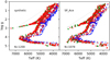 |
Fig. 4. Left: distribution of the mock populations on the (Teff, log g) plane synthesized with constant continuum opacity. The spectra have resolution R = 12 000 and S/N = 100. Right: Teff and log g of the spectra as derived by SP_Ace with constant continuum opacity. The blue points, red crosses, and green triangles represent the thin disk, halo/thick disk, and accreted stars, respectively. The solid, dashed, and dotted black lines show isochrones at [M/H] = 0.0 dex and 5 Gyr, [M/H] = −1.0 dex and 10 Gyr, and [M/H] = −2.0 dex and 10 Gyr, respectively. The light gray error bars represent the confidence intervals of the individual measurements. |
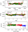 |
Fig. 5. Residuals between derived and reference parameters (y-axis) as a function of the reference parameters (x-axis) for spectra with constant continuum opacity, resolution R = 12 000 and S/N = 100. The full residual plot is reported in Fig. C.1. Symbols and colors are as in Fig. 4. |
6.1.2. Synthetic spectra with continuum opacity change
For the second test we synthesized the same sample of spectra by feeding SPECTRUM with the abundance file containing the elemental abundances. In this way we allowed SPECTRUM to internally recompute the continuum opacity. The first SP_Ace results on these spectra (not presented here) showed increased dispersion and systematic errors, in particular for alpha-enhanced spectra. The cause of these larger dispersion and systematic errors is the increased continuum opacity triggered by the enhancement of the α-elements, which was not taken into account during the construction of the GCOG library.
In order to reduce the errors and to account for the increased continuum opacity in the alpha-enhanced spectra, we adopted the following correction. An alpha abundant atmosphere has a greater opacity comparable to a higher nominal metallicity, as reported by Salaris et al. (1993), who proposed a formula to compute the correspondent metallicity when the relative abundance [α/Fe] is known. Therefore, we added a few lines into the SP_Ace code to allow it to change the GCOG nominal metallicity as a function of the alpha-enhancement detected during the measurement process following the Salaris formula (see Eq. (1)) where the alpha-enhancement [α/Fe] is internally computed on the fly by SP_Ace as the average of the relative abundances [El/Fe] of the elements C, O, Mg, Si, Ca, and Ti9. With this version of SP_Ace the resulting stellar parameters show reduced errors and systematics. These results are presented in Fig. 6 and Fig. 7 (see Fig. C.2 for the full residual comparison). The relative abundances [El/Fe] obtained are shown in Fig. C.3.
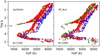 |
Fig. 6. As in Fig. 4, but for spectra synthesized with variable continuum opacity and measured with SP_Ace adopting the metallicity Salaris correction. |
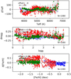 |
Fig. 7. As in Fig. 5, but for spectra synthesized with variable continuum opacity and measured with SP_Ace adopting the metallicity Salaris correction. For the full residual plot see Fig. C.2. |
6.1.3. Discussion
The new version of SP_Ace shows improved performance on stellar parameters, whose residuals in Fig. C.1 have smaller dispersions and trends with respect to the previous SP_Ace version. This result obtained on synthetic spectra without continuum opacity change proves the good ability of SP_Ace to build a spectrum model that looks much like a synthetic one, thanks to its improved features.
However, when we let SPECTRUM change the continuum opacity (synthesizing spectra that are therefore expected to look more realistic) the SP_Ace results are not as good as before because the weakening of the lines due to the continuum opacity change was neglected during the construction of the GCOG library. At the present time this effect cannot be taken in account without big changes in the GCOG library construction. To do so we would need to add one more variable (atmosphere alpha-enhancement) to the four variables (Teff, log g, [M/H], [El/M]) already considered in the GCOG library, making the construction of the library (and the SP_Ace analysis procedure) more complex. The correction to this problem that we proposed in the previous section provides some improvements, although it cannot fully remove some systematic errors. In the present version this is the best possible solution to minimize such errors.
Despite the errors just discussed, the results on the (Teff, log g) plane seen in Fig. 6 show a good distribution of the SP_Ace parameters that follow the isochrones fairly well. The derived elemental abundances are also satisfactory (Fig. C.3), showing the three populations neatly separated and following the expected sequences for nearly all the elements. Elemental abundance error size changes naturally for different elements because of the different number of absorption lines present in the spectra. This implies that the lower the number of lines seen (therefore measurable), the lower the accuracy of the correspondent elemental abundance.
6.2. Real spectra
We ran SP_Ace on 442 real spectra, collected from the S4N catalog (Allende Prieto et al. 2004), the ELODIE spectral library (Prugniel et al. 2007), and the spectra of the benchmark stars (Jofré et al. 2014). These spectra are the same as used in Paper I, where the interested reader can find further details. These collections of spectra provide precise stellar parameters and elemental abundances that we can use as reference to estimate SP_Ace’s accuracy and precision. The original spectra, that have very high resolution and S/N, were degraded to resolution R = 12 000 and S/N = 100 for the purposes of the present test. The measurements were performed with SP_Ace over the wavelength interval 4800−6270 Å and 6310−6860 Å in order to avoid the interval 6270−6310 Å affected by telluric lines. The resulting stellar parameters compared to the reference parameters on the (Teff, log g) plane are shown in Fig. 8, while the residuals are shown in Fig. 9 (see Fig. D.1 for the full plot). The SP_Ace abundances are reported in Fig. D.2 with one-to-one comparisons to the reference values.
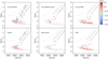 |
Fig. 8. Distribution on the (Teff, log g) plane of the reference (bottom) and the resulting SP_Ace parameters (top) of the three different sets ELODIE, Benchmark, and S4N (from left to right) at resolution R = 12 000 and S/N = 100. Isochrones as in Fig. 4 are reported as reference. |
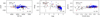 |
Fig. 9. Residuals (SP_Ace minus reference) of the stellar parameters Teff, log g, and [Fe/H] for the star sets of ELODIE (black points), S4N (blue triangles), and Benchmark (red crosses) for resolution R = 12 000 and S/N = 100. The reported statistics are computed for the three sets all together. The full comparison of residual parameters is shown in Fig. D.1. |
6.2.1. Discussion
We begin our discussion of the expected errors in stellar parameters and elemental abundances recalling that, in the case of real spectra, the dispersion of the residuals measured minus expected is the quadratic sums of the dispersion of the SP_Ace measurements and the dispersion of the measurements reported in the ELODIE, S4N, and Benchmark catalogs. Given that these catalogs measurements of real spectra, and that errors affect them too, we must keep in mind that the dispersions reported in our comparisons must be considered as upper limits of the errors expected from SP_Ace.
The distributions on the (Teff, log g) plane are shown in Fig. 8 for the three catalogs separately. The SP_Ace stellar parameters follow fairly well the isochrones, although there is a tendency to underestimate the gravity for dwarf stars when these are compared to the positions of the isochrones. This systematic error affects the ELODIE reference values too, while the S4N and Benchmark stars are unaffected. This can be easily explained. While the SP_Ace and the ELODIE log g are spectroscopically derived, the log g s of S4N and Benchmark stars are computed from the fundamental relation g = GM/R2 where the radius R was obtained from angular and parallaxes measurements, while the mass M was derived from the evolutionary tracks. Thus, they naturally lie on the isochrones.
For better statistics, we decided to measure all the spectra of the ELODIE catalog. Because not all the ELODIE stellar parameters are of high quality, we limit our comparison to the distribution of the results in the (Teff, log g) plane with respect to the isochrones. The distribution presented in Fig. 10 shows a good performance of SP_Ace for dwarfs stars, whose sequence closely follows the slope of the isochrones, albeit slightly underestimated in log g. However, there are some systematics. The red clump stars, seen as an overdensity at log g ∼ 2.6 in the ELODIE data (top panel), are instead found at log g ∼ 3 in the SP_Ace results (bottom panel), revealing the overestimation of the gravity in this area of the stellar parameters. Cool dwarf stars (Teff < 4500 K) show too low log g s with lower Teff.
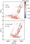 |
Fig. 10. Distribution on the (Teff, log g) plane of the whole ELODIE catalog (top) and the resulting SP_Ace parameters (bottom) for resolution R = 12 000 and S/N = 100. Isochrones as in Fig. 4 are reported as reference. |
For giant stars (log g < 2) the SP_Ace gravity is slightly overestimated (see central panel of Fig. 9). Metal-poor dwarf stars show a systematic underestimation in all three parameters Teff, log g, and [Fe/H] (see right panels of Fig. D.1). The spectra of these kinds of stars hold less information because their absorption lines are fewer and weaker than in others stars; therefore, they are prone to larger stochastic and systematic errors.
In Fig. 11 we report the standard deviations of the stellar parameters residuals (SP_Ace minus reference) of the real spectra data sets for different S/N and spectral resolutions. Computed in this way, the standard deviations σ represent an estimate of the stochastic errors expected by SP_Ace. As said before, these are upper limits since they are the quadratic sums of the SP_Ace and the reference errors. However, we have to keep in mind that stochastic errors depend on the stellar parameters, typically smaller for spectra rich in absorption lines (such as metal-rich giant stars) and larger for spectra poor of lines (metal-poor hot dwarfs). The errors reported in Fig. 11 must therefore be taken as a rough overall estimation.
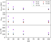 |
Fig. 11. Standard deviations of the residuals of the stellar parameters Teff, log g, and [Fe/H] (SP_Ace minus reference) of the real spectra data sets for different S/N and spectral resolutions R. |
6.2.2. Elemental abundances quality
One-to-one comparison of the SP_Ace abundances versus the reference values are reported in Fig. D.2 together with offsets and dispersions for the two data sets of the benchmark and S4N stars (the ELODIE catalog does not report abundances). The residual dispersions are between 0.05 and 0.2 dex, depending on the element considered, with offsets that can differ for the two data sets. We note that the discrepancies between the S4N and SP_Ace abundances for Sc and Ti observed in Paper I are still present. On the other hand, the same two elements do not show significant discrepancies when compared to the benchmark stars, which disagree with the same S4N abundances as well. The discrepancies can be due to different solar abundances adopted or to a systematic difference in oscillator strengths of the absorption lines set adopted in these two catalogs. A similar discrepancy is also observed for Co.
However, observing the relative abundance distributions on Fig. D.3, we see that some of the elements do not seem reliable. We decided to classify the elements with three quality labels, depending to their dispersion/systematic errors in Fig. D.2 and the meaningfulness of their distributions in the ([El/Fe], [Fe/H]) plane where they should reproduce the typical distributions observed in the Galaxy. The labels are given as follows:
First quality: Mg, Si, Ca, Sc, Ti, V, Cr, Mn, Co, Ni, Cu
Second quality: C, Na, Al, Zn, Ba, La
Third quality: Y, Zr, Ce, Nd
We decided to reject O, Pr, and Sm because they show no clear sequence and exhibit large dispersions. We note that these quality labels are valid only for the wavelength considered for the presented tests. The quality of the abundance of an element strongly depends on the number of elemental lines measured which, in turn, depends on the wavelength range chosen, the S/N of the spectrum, and the metallicity range of the star. In our tests we covered the whole possible wavelength range and considered high-quality spectra. For real spectral surveys, the conditions are often worse. Therefore, we invite the user to evaluate the element abundance quality in its actual working conditions.
From the tests on synthetic and real spectra, we can conclude that SP_Ace derives reliable stellar parameters for FGK type stars in the high to intermediate metallicity range.
7. Conclusions
We presented a new version of SP_Ace, a code for the automated measurement of stellar parameters and elemental abundances. This work, although oriented to provide a general purpose tool for spectral analysis, was triggered by our willingness to apply SP_Ace to the spectra of the coming WEAVE spectroscopic survey (Dalton et al. 2014), which oriented the choice of wavelength coverage of the new GCOG library.
This version (v1.4) underwent many updates, the main ones summarized by the following points:
We created a new GCOG library covering the wavelength range 4800−6860 Å (extended to the blue with respect to the previous version, to satisfy the need to measure the blue/green WEAVE spectra);
We refined the GCOG library by an improved correction of the opacity of the neighboring lines;
We implemented a new line profile, covering the spectral resolution range of R = 2000−40 000.
With this new version we see an improved accuracy and precision with respect to the previous version of SP_Ace on synthetic spectra with constant continuum opacity. However, on real spectra we do not see clear improvements, nor a worsening. Since SP_Ace tries to create a spectrum model as close as possible to a synthetic one, the lack of a clear improvement with real spectra may be due to the difference between synthetic and real spectra because the unrealistic features of the 2D atmosphere models, neglected NLTE effects, and/or molecular bands that are not modeled by SP_Ace. However, the distributions of the stars on the (Teff, log g) plane by SP_Ace look realistic with some identified systematic errors. Similarly realistic distributions are shown by the elemental abundances relative to the iron abundance. We can conclude that SP_Ace derives reliable stellar parameters for FGK-type stars in the high to intermediate metallicity range.
Although the extension of the GCOG library was triggered by the coming WEAVE spectroscopic survey, the present version 1.4 of the SP_Ace code and its new GCOG library released with this work is designed for general purposes. The customized version of SP_Ace for the WEAVE spectra will be presented in a future work.
The limits in resolution we suggest are due to the capabilities of SP_Ace in reproducing the line profile, which is not satisfactory at very high resolution.
In Paper I we suggested limiting the analysis to spectra with resolution between 2000 and 20 000, although in this work we extended the usable resolution to 40 000.
This range is usually small, and corresponds to a wavelength shift of ±1 full width half maximum of the line profile.
When queried for specific stellar parameters, the VALD interface returns results given by the closest atmosphere model. In these cases VALD was queried with the following model atmospheres: castelli_ap00k2_T05750G45.krz for the Sun, castelli_ap00k2_T04250G15.krz for Arcturus, castelli_ap00k2_T06500G40.krz for Procyon. For the Arcturus atmosphere we chose to use a higher metallicity to also get those weak lines that would not be visible at Arcturus abundance [Fe/H] = −0.52 dex.
It is possible to constrain the elemental abundances during the log gf calibration, although this is true in most of the cases but not all. See discussion in Sect. 4 of Paper I.
This method is employed by the calibration routine and SP_Ace as well.
As total χ2 we mean the sum of the χ2 values of the five standard spectra.
These element abundances may not be measurable in any spectrum. Therefore, the [α/Fe] is computed as the mean of the elements available.
We neglected lines having strength weaker than 0.1 in all the normalized standard spectra seen in Sect. 3.2.
Acknowledgments
B. C. wants to thanks H.-G. Ludwig for bringing to his attention the work of Sennhauser et al. where the present correction for the opacity of the neighbors lines was inferred from. B. C. also thanks the author of SPECTRUM R. O. Gray for useful explanations on how SPECTRUM works.
References
- Adibekyan, V. Z., Sousa, S. G., Santos, N. C., et al. 2012, A&A, 545, A32 [NASA ADS] [CrossRef] [EDP Sciences] [Google Scholar]
- Aguado, D. S., González Hernández, J. I., Allende Prieto, C., & Rebolo, R. 2017, A&A, 605, A40 [CrossRef] [EDP Sciences] [Google Scholar]
- Allende Prieto, C., Barklem, P. S., Lambert, D. L., & Cunha, K. 2004, A&A, 420, 183 [NASA ADS] [CrossRef] [EDP Sciences] [Google Scholar]
- Beers, T. C., Lee, Y., Sivarani, T., Allende Prieto, C., & SEGUE Calibration Team 2006, Mem. Soc. Astron. It., 77, 1171 [Google Scholar]
- Bensby, T., Feltzing, S., & Oey, M. S. 2014, A&A, 562, A71 [NASA ADS] [CrossRef] [EDP Sciences] [Google Scholar]
- Blanco-Cuaresma, S., Soubiran, C., Jofré, P., & Heiter, U. 2014, A&A, 566, A98 [NASA ADS] [CrossRef] [EDP Sciences] [Google Scholar]
- Boeche, C., & Grebel, E. K. 2016, A&A, 587, A2 [NASA ADS] [CrossRef] [EDP Sciences] [Google Scholar]
- Boeche, C., Siebert, A., Williams, M., et al. 2011, AJ, 142, 193 [NASA ADS] [CrossRef] [Google Scholar]
- Boeche, C., Smith, M. C., Grebel, E. K., et al. 2018, AJ, 115, 188 [Google Scholar]
- Bressan, A., Marigo, P., Girardi, L., et al. 2012, MNRAS, 427, 127 [NASA ADS] [CrossRef] [Google Scholar]
- Castelli, F., & Kurucz, R. L. 2003, in Modelling of Stellar Atmospheres, eds. N. Piskunov, W. W. Wiess, & D. F. Gray, IAUS Symp., 210, 20, Published on behalf of the IAU by the ASP [Google Scholar]
- Chen, Y., Bressan, A., Girardi, L., et al. 2015, MNRAS, 452, 1068 [NASA ADS] [CrossRef] [Google Scholar]
- Cirasuolo, M., Afonso, J., Carollo, M., et al. 2014, Proc. SPIE, 91470N [Google Scholar]
- Dalton, G., Trager, S., Abrams, D. C., et al. 2014, Proc. SPIE, 91470L [Google Scholar]
- de Jong, R. S., Agertz, O., Berbel, A. A., et al. 2019, Messenger, 175, 3 [Google Scholar]
- DESI Collaboration 2016, ArXiv e-prints [arXiv:1611.00036] [Google Scholar]
- Freeman, K. C. 2012, in Galactic Archaeology: Near-Field Cosmology and the Formation of the Milky Way, eds. W. Aoki, M. Ishigaki, T. Suda, T. Tsujimoto, & N. Arimoto, ASP Conf. Ser., 458, 393 [Google Scholar]
- Gaia Collaboration (Brown, A., et al.) 2018, A&A, 616, A1 [NASA ADS] [CrossRef] [EDP Sciences] [Google Scholar]
- Gilmore, G., Randich, S., Asplund, M., et al. 2012, Messenger, 147, 25 [Google Scholar]
- Gray, R. O., & Corbally, C. J. 1994, AJ, 107, 742 [Google Scholar]
- Grevesse, N., & Sauval, A. J. 1998, Space Sci. Rev., 85, 161 [Google Scholar]
- Grevesse, N., Asplund, M., & Sauval, A. J. 2007, Space Sci. Rev., 130 [Google Scholar]
- Hinkle, K., Wallace, L., Harmer, D., Ayres, T., & Valenti, J. 2000, in Visible and Near Infrared Atlas of the Arcturus Spectrum 3727–9300 Å, IAU Joint Discuss., 1, ftp://ftp.noao.edu/catalogs/arcturusatlas/visual [Google Scholar]
- Jofré, P., Heiter, U., Soubiran, C., et al. 2014, A&A, 564, A133 [NASA ADS] [CrossRef] [EDP Sciences] [Google Scholar]
- Jofré, P., Heiter, U., Soubiran, C., et al. 2015, A&A, 582, A81 [NASA ADS] [CrossRef] [EDP Sciences] [Google Scholar]
- Kramida, A., Ralchenko, Y., Reader, J., & NIST ASD Team 2013, NIST Atomic Spectra Database (ver. 5.1) (Gaithersburg, MD: National Institute of Standards and Technology), http://physics.nist.gov/asd [Google Scholar]
- Kollmeier, J. A., Zasowski, G., Rix, H. W., et al. 2017, ArXiv e-prints [arXiv:1711.03234] [Google Scholar]
- Kupka, F., Piskunov, N., Ryabchikova, T. A., Stempels, H. C., & Weiss, W. W. 1999, A&AS, 138, 119 [NASA ADS] [CrossRef] [EDP Sciences] [MathSciNet] [PubMed] [Google Scholar]
- Kurucz, R. L. 1995, in Astrophysical Application of Powerful New Database, eds. S. J. Adelman, & W. L. Wiese, ASP Conf. Ser., 78, 205, (San Francisco, CA) [Google Scholar]
- Laverick, M., Lobel, A., Royer, P., et al. 2019, A&A, 624, A60 [NASA ADS] [CrossRef] [EDP Sciences] [Google Scholar]
- Majewski, S. R. 2012, in American Astronomical Society Meeting Abstracts, Am. Astron. Soc. Meeting Abstr., 219, 205.06 [Google Scholar]
- McLean, A. B., Mitchell, C. E. J., & Swanston, D. M. 1994, J. Electron Spectrosc. Relat. Phenom., 69, 125 [CrossRef] [Google Scholar]
- Newberg, H. J., Carlin, J. L., Chen, L., & Lamost-Plus Partnership 2012, in Galactic Archaeology:Near-Field Cosmology and the Formation of the Milky Way, eds. W. Aoki, M. Ishigaki, T. Suda, T. Tsujimoto, & N. Arimoto, ASP Conf. Ser., 458, 405 [Google Scholar]
- Pedregosa, F., Varoquaux, G., Gramfort, A., et al. 2011, Scikit-learn: Machine Learning in Python, JMLR 12, 2825 [Google Scholar]
- Prugniel, P., Soubiran, C., Koleva, M., & Le Borgne, D. 2007, VizieR Online Data Catalog, 3251 [Google Scholar]
- Ramírez, I., & Allende Prieto, C. 2011, ApJ, 743, 135 [NASA ADS] [CrossRef] [Google Scholar]
- Salaris, M., Chieffi, A., & Straniero, O. 1993, ApJ, 414, 580 [NASA ADS] [CrossRef] [Google Scholar]
- Sennhauser, C., Berdyugina, S. V., & Fluri, D. M. 2009, A&A, 507, 1711 [NASA ADS] [CrossRef] [EDP Sciences] [Google Scholar]
- Sneden, C. 1973, PhD thesis, Univ. Texas at Austin, USA [Google Scholar]
- Steinmetz, M., Zwitter, T., Siebert, A., et al. 2006, AJ, 132, 1645 [Google Scholar]
- Valentini, M., Chiappini, C., Davies, G. R., et al. 2017, A&A, 600, A66 [NASA ADS] [CrossRef] [EDP Sciences] [Google Scholar]
Appendix A: The “guess line” method
In the wavelength interval considered, there are unidentified absorption lines. For the method SP_Ace employs to estimate the stellar parameters, these unidentified lines can affect the results when such lines are instrumentally or physically blended with other lines because they lead to systematic deviations of the expected strength of the blends. Even a rough estimate of their strength can reduce a systematic error. Therefore, we developed a method to guess the excitation potential, log gf, and the element that an unidentified absorption line belongs to. This method relies on a machine learning (ML) algorithm. We describe how it works here.
After a first log gf calibration, the calibrating software has an internal line list containing thousands of lines for which we know the atomic species El, the low excitation potential χl, the calibrated log gf, and the EWs of the line’s best matching synthetic spectra for the five different standard stars. It is reasonable to assume that if two absorption lines have the same EW on the five standard spectra, they should share the same χl and the same log gf. For the latter this is true under the hypothesis of the correctness of the abundance of the element the line belongs to. We can reasonably assume that the chosen abundances of the standard stars are close to the truth. However, the entanglement between log g and the abundance of the element the line belongs to (which is unknown) is not fully solved. Therefore, the element found by this method may be not the right one, but when this line shows a good match with the correspondent lines of all the five standard spectra we can assume that this line (considered a “dummy” line) parrots the observed unknown line through the parameter space, helping to minimize the systematic error. As said, this is an empiric method and must be considered experimental.
We prepared a training set as table which rows (one for each absorption line) contain five EWs (the EW of the line for each standard star), while the target set contains the El, χl, and log gf values for each line. We decided to use a very simple ML algorithm such as the nearest neighbors algorithm (from the Python scikit-learn package; Pedregosa et al. 2011). Once the ML model has been trained, the user inputs the central wavelength λ of the unknown line and the software measures its EWs for the five observed standard spectra by assuming a Gaussian profile. Then, these five measured EWs and the ML model are used to find the closest line’s atomic species, χl, and the log gf. The last atomic parameter we need to guess is the high excitation potential χh, expressed in cm−1, which is computed as
where λ is the line wavelength expressed in Å. The software proposes five different choices that correspond to the five closest neighbors found by the ML model. The choice is left to the user.
Appendix B: The SP_Ace line profile
SP_Ace employs the Voigt line profile by McLean et al. (1994), which is a function of the parameters γG and γL. As a first approximation the width of the Gaussian part of the line (the core of the line, expressed by γG) is driven by the spectral resolution, while the width of the line wings (expressed by γL) is a function of the stellar parameters, in addition to the other spectral parameters. After some investigation we chose these parameters: EW, γG (spectral resolution), log g, and Teff.
To derive this function we first fit 3189 lines10 of the line list with the McLean profile at the optimal match found with a χ2 minimization routine. The absorption lines were synthesized with the same software and atmosphere models used to build the EW library (see Sect. 4) for a stellar parameter grid with points [3600, 4800, 6000, 7400] K in Teff, [0.6, 3.0, 4.2, 5.0] in log g, [0.0, −0.4, −1.0, −2.0] dex in [M/H], and for the spectral resolutions R = 2000, 5000, 12 000, 20 000, 40 000. This provided a large sample of γG and γL parameters of the Voigt profiles that fits best the absorption lines at the different resolutions and atmosphere conditions. By using this sample, we extracted a general (polynomial) law for γL as a function of EW, γG, log g, and Teff. This is a second-degree polynomial function:
 (B.1)
(B.1)
In Fig. B.1 we show γL for spectral resolution R = 5000 and 20 000 and their polynomial approximations as a function of log g. The polynomial law was obtained by considering all the lines except Hα, Hβ, and the Na I doublet lines (at 5889 and 5895 Å) because they do not behave as the other lines.
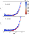 |
Fig. B.1. Lorentzian width γL of 3189 absorption lines in 64 different stellar atmospheres and spectra resolutions R = 5000 (top) and R = 20 000 (bottom). The color bar represents the gravity log g. The dotted light blue and solid blue lines show the polynomial γL for dwarf stars (Teff = 6000 K log g = 4.2 and Teff = 3600 K log g = 5.0, respectively). The dashed red line shows the polynomial γL for a giant star with Teff = 3600 K and log g = 0.6. |
On the other hand, the Gaussian γG remains constant up to EW ∼ 1000 mÅ and then, when the core of the line is saturated, it seems to rise linearly with a slope that differs for different spectral resolutions. After some tests we decided to not reproduce this behavior and to use a constant γG because using a polynomial function improved the cores of a handful of intense lines and did not bring any improvement in the stellar parameter estimates.
Appendix C: Synthetic spectra results
In this section we show the full figures that in Sect. 6.1.2 were not reported or were only partially reported. In Fig. C.1 we show the residuals between measured and expected stellar parameters for synthetic spectra synthesized with SPECTRUM and no continuum opacity change (as MOOG would) and no Salaris correction applied in the SP_Ace code. This figure can be directly compared to Fig. 17 of Paper I where the spectra were synthesized with MOOG and the stellar parameters were derived without Salaris correction. We can see that the new SP_Ace code has an improved accuracy in deriving the stellar parameters. However, by synthesizing the spectra with SPECTRUM (which modifies the continuum opacity as a function of the elemental abundances) and applying the Salaris correction in SP_Ace, the accuracy decrease as shown in Fig. C.2. The obtained elemental abundances with respect to the expected ones are reported in Fig. C.3.
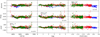 |
Fig. C.1. Residuals between derived and reference parameters (y-axis) as a function of the reference parameters (x-axis) for spectra with constant continuum opacity. This is the complete figure that was only partially shown in Fig. 5. Symbols and colors are as in Fig. 4. |
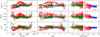 |
Fig. C.2. Residuals between derived and reference parameters (y-axis) as a function of the reference parameters (x-axis) for spectra with variable continuum opacity and SP_Ace metallicity Salaris correction. This is the complete figure that was only partially shown in Fig. 7. Symbols and colors are as in Fig. 4. |
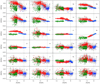 |
Fig. C.3. Chemical abundance distribution measured by SP_Ace for spectra with variable continuum opacity and SP_Ace metallicity Salaris correction. The expected distributions are shown by the colored solid lines. Symbols and colors are as in Fig. 4. |
Appendix D: Real spectra results
In this section we show the figures that were not reported or were only partially reported in Sect. 6.2. In Fig. D.1 we show the residuals between measured and expected stellar parameters for the set of real spectra described in Sect. 6.2. The stellar parameters were derived here using the Salaris correction in SP_Ace. From these measurements we obtained elemental abundances that are compared with the reference abundances Fig. D.2. In Fig. D.3 we show how these abundances distribute relatively to iron.
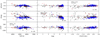 |
Fig. D.1. Residuals (SP_Ace minus reference) of the stellar parameters Teff, log g, and [Fe/H] for the star sets of ELODIE (black points), S4N (blue triangles), and benchmark (red crosses). The reported statistics are computed for the three sets all together. |
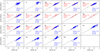 |
Fig. D.2. Comparison between the reference abundances (x-axis) and the values measured by SP_Ace (y-axis) for the S4N (blue triangles) and the Benchmark (red crosses) stars. In blue and red we report the statistics for the two sets, respectively. |
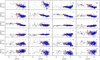 |
Fig. D.3. Distributions of the relative abundances [El/Fe] of all the elements measured by SP_Ace. Symbols are as in Fig. D.1. |
All Tables
Effective temperature (K), gravity, metallicity (dex), micro- and macro-turbulence (in km s−1) adopted to synthesize the spectra of the standard stars.
Instrumental FWHMs adopted for the synthetic spectra in the four wavelength ranges.
Final chemical abundances for the five stars derived as result of the log gf calibration.
Iron abundance ranges, and coefficients m and q of the linear law [El/Fe] = m ⋅ [Fe/H] + q that express the chemical abundances used to synthesize the spectra of the three mock stellar populations.
All Figures
|
Fig. 1. Distributions of the NEWRs of the elements Si and Fe as a function of their EW for the five standard stars before (left) and after (right) the calibration. The standard stars are indicated by different colors (from top to bottom): the Sun (yellow), Arcturus (red), Procyon (blue), ϵ Vi (green), and ϵ Eri (purple). The triangles represent lines for which NEWR is larger than +0.4 or smaller than −0.4. In each panel the mean and the Pearson correlation parameter r are shown. |
| In the text | |
|
Fig. 2. Comparison between the calibrated log gf values (y-axis) and those of three different databases. Left: comparison with the VALD values for calibrated lines used for the final GCOG library. Center: comparison with the NIST values that have an estimated accuracy lower than 10% of the gf-value. Right: comparison with the BRASS values obtained with the grid method for Fe lines only. The statistics were computed on the residuals calibrated minus original log gf after a 3σ clipping. |
| In the text | |
|
Fig. 3. Residual between the EWs in the EW library and that obtained from the GCOG library, expressed in abundance dex for lines with EW > 1 mÅ for three different atmosphere parameters. Red crosses, gray points, and blue triangles represent the EWs for the abundances [El/M] = +0.2, 0.0, and −0.2 dex, respectively. |
| In the text | |
|
Fig. 4. Left: distribution of the mock populations on the (Teff, log g) plane synthesized with constant continuum opacity. The spectra have resolution R = 12 000 and S/N = 100. Right: Teff and log g of the spectra as derived by SP_Ace with constant continuum opacity. The blue points, red crosses, and green triangles represent the thin disk, halo/thick disk, and accreted stars, respectively. The solid, dashed, and dotted black lines show isochrones at [M/H] = 0.0 dex and 5 Gyr, [M/H] = −1.0 dex and 10 Gyr, and [M/H] = −2.0 dex and 10 Gyr, respectively. The light gray error bars represent the confidence intervals of the individual measurements. |
| In the text | |
|
Fig. 5. Residuals between derived and reference parameters (y-axis) as a function of the reference parameters (x-axis) for spectra with constant continuum opacity, resolution R = 12 000 and S/N = 100. The full residual plot is reported in Fig. C.1. Symbols and colors are as in Fig. 4. |
| In the text | |
|
Fig. 6. As in Fig. 4, but for spectra synthesized with variable continuum opacity and measured with SP_Ace adopting the metallicity Salaris correction. |
| In the text | |
|
Fig. 7. As in Fig. 5, but for spectra synthesized with variable continuum opacity and measured with SP_Ace adopting the metallicity Salaris correction. For the full residual plot see Fig. C.2. |
| In the text | |
|
Fig. 8. Distribution on the (Teff, log g) plane of the reference (bottom) and the resulting SP_Ace parameters (top) of the three different sets ELODIE, Benchmark, and S4N (from left to right) at resolution R = 12 000 and S/N = 100. Isochrones as in Fig. 4 are reported as reference. |
| In the text | |
|
Fig. 9. Residuals (SP_Ace minus reference) of the stellar parameters Teff, log g, and [Fe/H] for the star sets of ELODIE (black points), S4N (blue triangles), and Benchmark (red crosses) for resolution R = 12 000 and S/N = 100. The reported statistics are computed for the three sets all together. The full comparison of residual parameters is shown in Fig. D.1. |
| In the text | |
|
Fig. 10. Distribution on the (Teff, log g) plane of the whole ELODIE catalog (top) and the resulting SP_Ace parameters (bottom) for resolution R = 12 000 and S/N = 100. Isochrones as in Fig. 4 are reported as reference. |
| In the text | |
|
Fig. 11. Standard deviations of the residuals of the stellar parameters Teff, log g, and [Fe/H] (SP_Ace minus reference) of the real spectra data sets for different S/N and spectral resolutions R. |
| In the text | |
|
Fig. B.1. Lorentzian width γL of 3189 absorption lines in 64 different stellar atmospheres and spectra resolutions R = 5000 (top) and R = 20 000 (bottom). The color bar represents the gravity log g. The dotted light blue and solid blue lines show the polynomial γL for dwarf stars (Teff = 6000 K log g = 4.2 and Teff = 3600 K log g = 5.0, respectively). The dashed red line shows the polynomial γL for a giant star with Teff = 3600 K and log g = 0.6. |
| In the text | |
|
Fig. C.1. Residuals between derived and reference parameters (y-axis) as a function of the reference parameters (x-axis) for spectra with constant continuum opacity. This is the complete figure that was only partially shown in Fig. 5. Symbols and colors are as in Fig. 4. |
| In the text | |
|
Fig. C.2. Residuals between derived and reference parameters (y-axis) as a function of the reference parameters (x-axis) for spectra with variable continuum opacity and SP_Ace metallicity Salaris correction. This is the complete figure that was only partially shown in Fig. 7. Symbols and colors are as in Fig. 4. |
| In the text | |
|
Fig. C.3. Chemical abundance distribution measured by SP_Ace for spectra with variable continuum opacity and SP_Ace metallicity Salaris correction. The expected distributions are shown by the colored solid lines. Symbols and colors are as in Fig. 4. |
| In the text | |
|
Fig. D.1. Residuals (SP_Ace minus reference) of the stellar parameters Teff, log g, and [Fe/H] for the star sets of ELODIE (black points), S4N (blue triangles), and benchmark (red crosses). The reported statistics are computed for the three sets all together. |
| In the text | |
|
Fig. D.2. Comparison between the reference abundances (x-axis) and the values measured by SP_Ace (y-axis) for the S4N (blue triangles) and the Benchmark (red crosses) stars. In blue and red we report the statistics for the two sets, respectively. |
| In the text | |
|
Fig. D.3. Distributions of the relative abundances [El/Fe] of all the elements measured by SP_Ace. Symbols are as in Fig. D.1. |
| In the text | |
Current usage metrics show cumulative count of Article Views (full-text article views including HTML views, PDF and ePub downloads, according to the available data) and Abstracts Views on Vision4Press platform.
Data correspond to usage on the plateform after 2015. The current usage metrics is available 48-96 hours after online publication and is updated daily on week days.
Initial download of the metrics may take a while.