| Issue |
A&A
Volume 645, January 2021
|
|
|---|---|---|
| Article Number | A79 | |
| Number of page(s) | 23 | |
| Section | Planets and planetary systems | |
| DOI | https://doi.org/10.1051/0004-6361/202038361 | |
| Published online | 18 January 2021 | |
Evidence of three mechanisms explaining the radius anomaly of hot Jupiters
1
Physikalisches Institut, Universität Bern,
Gesellschaftsstrasse 6,
3012 Bern, Switzerland
e-mail: This email address is being protected from spambots. You need JavaScript enabled to view it.
2
Max-Planck-Institut für Astronomie,
Königstuhl 17,
Heidelberg 69117, Germany
3
Institut für Astronomie und Astrophysik, Universität Tübingen,
Auf der Morgenstelle 10,
72076 Tübingen, Germany
Received:
6
May
2020
Accepted:
4
September
2020
Abstract
Context. The anomalously large radii of hot Jupiters are still not fully understood, and all of the proposed explanations are based on the idea that these close-in giant planets possess hot interiors. Most of the mechanisms proposed have been tested on a handful of exoplanets.
Aims. We approach the radius anomaly problem by adopting a statistical approach. We want to infer the internal luminosity for the sample of hot Jupiters, study its effect on the interior structure, and put constraints on which mechanism is the dominant one.
Methods. We developed a flexible and robust hierarchical Bayesian model that couples the interior structure of exoplanets to the observed properties of close-in giant planets. We applied the model to 314 hot Jupiters and inferred the internal luminosity distribution for each planet and studied at the population level (i) the mass–luminosity–radius distribution and as a function of equilibrium temperature the distributions of the (ii) heating efficiency, (iii) internal temperature, and the (iv) pressure of the radiative–convective–boundary (RCB).
Results. We find that hot Jupiters tend to have high internal luminosity with 104 LJ for the largest planets. As a result, we show that all the inflated planets have hot interiors with an internal temperature ranging from 200 up to 800 K for the most irradiated ones. This has important consequences on the cooling rate and we find that the RCB is located at low pressures between 3 and 100 bar. Assuming that the ultimate source of the extra heating is the irradiation from the host star, we also illustrate that the heating efficiency increases with increasing equilibrium temperature and reaches a maximum of 2.5% at ~1860 K, beyond which the efficiency decreases, which is in agreement with previous results. We discuss our findings in the context of the proposed heating mechanisms and illustrate that ohmic dissipation, the advection of potential temperature, and thermal tides are in agreement with certain trends inferred from our analysis and thus all three models can explain various aspects of the observations.
Conclusions. We provide new insights on the interior structure of hot Jupiters and show that with our current knowledge, it is still challenging to firmly identify the universal mechanism driving the inflated radii.
Key words: planets and satellites: gaseous planets / planets and satellites: interiors / planets and satellites: physical evolution
© P. Sarkis et al. 2021
 Open Access article, published by EDP Sciences, under the terms of the Creative Commons Attribution License (https://creativecommons.org/licenses/by/4.0), which permits unrestricted use, distribution, and reproduction in any medium, provided the original work is properly cited.
Open Access funding provided by Max Planck Society.
1 Introduction
Two decades of observational and theoretical exploration have revealed that the anomalously large radii of close-in transiting giant planets holds firmly (e.g., Laughlin et al. 2011; Weiss et al. 2013). The radii of hot Jupiters are larger than what is predicted by standard interior structure models (Guillot & Showman 2002). Observations reveal that there is a strong correlation between the observed radii and the stellar incident flux (e.g., Enoch et al. 2012), with a threshold around ~2 × 10⁸ erg s−1 cm−2, corresponding to an equilibrium temperature of about 1000 K (Demory & Seager 2011; Miller & Fortney 2011), below which the physical mechanism becomes inefficient. Sestovic et al. (2018) further demonstrate that the inflation extent is mass dependent, where the planets with the largest anomalous radii have masses less than ~ <1MJ.
Many investigations have been carried out in order to explain the discrepancy between the observations and theoretical models. The proposed mechanisms can be divided into two categories: (i) slowing down cooling and contraction or (ii) depositing extra heat into the interior. Burrows et al. (2007) showed that slowing down the cooling and thus delaying contraction can be achieved by increasing the atmospheric opacity. Another way to delay contraction is to reduce the heat transport efficiency due to compositional gradients (Chabrier & Baraffe 2007).
It is well established that heating up the interior of the planet increases its entropy and thus its radius (Arras & Bildsten 2006; Marleau & Cumming 2014). The source of heat is still not constrained and possible sources could be tidal dissipation of an eccentric orbit (e.g., Bodenheimer et al. 2001), advection of potential temperature, which is a consequence of the strong stellar irradiation (Tremblin et al. 2017; Sainsbury-Martinez et al. 2019), or dissipative processes powered by the stellar irradiation flux. The latter has received a lot of attention and the mechanism to transport a fraction of the stellar incident flux into the interior is still an open question. One mechanism is atmospheric circulation, which leads to the thermal dissipation of kinetic energy into the interior (Guillot & Showman 2002; Showman & Guillot 2002). Another mechanism is ohmic dissipation (Batygin & Stevenson 2010; Batygin et al. 2011; Perna et al. 2010a; Huang & Cumming 2012; Wu & Lithwick 2013; Ginzburg & Sari 2016), where the irradiation drives fast winds through the planet’s magnetic fields, giving rise to currents that dissipate ohmically in the interior. Other mechanisms are thermal tides (Arras & Socrates 2010) and the mechanical greenhouse (Youdin & Mitchell 2010).
Some of these mechanisms come with a lot of approximations and uncertainties. For example, an important uncertain parameter in atmospheric circulation, ohmic dissipation, and the advection of potential temperature is the wind speeds and the effect of magnetic drag in damping the winds (Perna et al. 2010a,b). Another uncertainty is how deep the wind zone extends, which is important to constrain the pressures at which the extra heat should be dissipated. Wu & Lithwick (2013) illustrate that if the wind zone is at shallow pressures, then a significantly larger heating efficiency is needed to achieve the same interior heating, compared to heating at deeper pressures. Komacek & Youdin (2017) argue that the extra heat should be deposited in the convective layers or at the radiative–convective–boundary (RCB), otherwise it is reradiated away. Huang & Cumming (2012) deposited the extra heat in the radiative layers and as a consequence show that the RCB moves to deeper pressures. Fortney et al. (2007) showed that the RCB is located at pressures of 1000 bar, where little is known about the wind speeds at such deep pressures. However, the Fortney et al. (2007) models were developed for irradiated planets and do not consider the high internal entropy that hot Jupiters are believed to possess.
All the mechanisms proposed have been tested and applied on single or a handful of planets. It is yet to be demonstrated that these mechanisms can explain the radii of all the observed hot Jupiters. Within this context, in this paper we approach the radius inflation problem from a statistical point of view, similar to the approach of Thorngren & Fortney (2018, hereafter TF18). We do not model any of the previously mentioned mechanisms but rely solely on the interior structure model and atmospheric model. We develop a hierarchical Bayesian model that allows us to couple the interior structure models to the observed physical properties of hot Jupiters while incorporating the measurement uncertainties. Our approach naturally accounts for non-Gaussian likelihoods. We first apply our model on the individual planets to infer the internal luminosity that reproduces the observed physical properties of hot Jupiters, namely radius, mass, and equilibrium temperature. Second, as a consequence of the high internal entropy, we find that the interior tends to be hot and show that the RCB moves to shallow pressures. Finally, we compare our findings to the proposed mechanisms and show that ohmic dissipation (Batygin & Stevenson 2010), advection of potential temperature (Tremblin et al. 2017), and thermal tides (Arras & Socrates 2010) can explain the anomalously large radii of hot Jupiters.
In a recent study, TF18 showed that the heating efficiency ϵ increases as a function of equilibrium temperatureuntil a maximum of ~2.5% is reached at around 1500 K, beyond which it decreases. The basic shape of ϵ(Teq) provides evidence for ohmic dissipation. Building on the functional form of ϵ(Teq), (Thorngren et al. 2019, hereafter T19) studied the effect of central heating on the interior structure of hot Jupiters and found that the internal temperature is much hotter than previous estimates, which pushes the RCB to lower pressures. Our approach is similar to TF18 but rather than modeling the extra heating as a function of ϵ, we do not assume explicitly a source for the extra heat. Instead, we consider the planet reached steady state and compute the internal luminosity given the planet mass, radius, and equilibrium temperature. The advantage of this approach is twofold: first, we can compare our results to heating mechanisms where the source of extra heat is not the stellar irradiation, and second, we self-consistently study the effect of high internal entropy on the interior structure of hot Jupiters, namely the internal temperature and pressure of the RCB. We note, however, that both approaches should lead to the same results. We also convert the internal luminosity to a heating efficiency ϵ and compare our results to TF18 in Sect. 6.3. We show that our results are qualitatively similar using a larger sample focused on FGK main-sequence stars and using an independent interior structure model.
The outline of this paper is as follows. Section 2 provides an overview of the sample selection criteria. In Sect. 3 we present the interior structure model used in this analysis. In Sect. 4 we outline the probabilistic framework used to link observations and theory and derive the basic equation which our method is based on (Eq. (28)). We validate the statistical model by applying it on synthetic planetary data set generated using the Generation III Bern global model in Sect. 5. Readers interested in the results can safely skip to Sect. 6 where we present the results of our analysis. We discuss the results and the shortcomings of our approach in Sect. 7 and conclude in Sect. 8.
2 Sample selection
For the purpose of our study, we required that all the planets have measured masses and radii. Sestovic et al. (2018) showed that the radii of planets with masses less than 0.37 MJ do not show a clear dependence on the stellar incident flux. Photoevaporation plays an important role in the evolution of such low-mass close-in planets (Owen & Jackson 2012; Jin et al. 2014). Baraffe et al. (2004) also showed that these planets are subject to undergo Roche-lobe overflow. We therefore restrict our analysis to planets with masses 0.37 < Mp < 13MJ with semi-major axis a < 0.1 au. In our study, we make no attempt to correct for selection effects where it is still challenging to detect “medium-inflated” hot Jupiters around F stars using ground-based surveys (see the discussion in Sect. 7.5).
Lopez & Fortney (2016) suggested that giant planets around stars leaving the main-sequence experience a high level of irradiation that could ultimately increase their radii. However, other studies argued that ohmic heating cannot reinflate planets after they have already cooled (Wu & Lithwick 2013; Ginzburg & Sari 2016). A handful of reinflated planets have been discovered around giant stars (Grunblatt et al. 2016, 2017; Hartman et al. 2016). Since different mechanisms can be at play around evolved stars, we exclude such planets and only consider hot Jupiters around solar-like stars. Specifically, we consider stars with stellar temperature T* = 4000−7000 K and surface gravity log g = 4−4.9.
The data was taken from the Transiting Extrasolar Planet Catalogue (TEPCat1; Southworth 2011), last accessed on November 2018. The aforementioned constraints on the planet mass, semi-major axis, and stellar temperature and surface gravity, lead to a final sample consisting of 314 hot Jupiters. The equilibrium temperature (Teq) values in the literature are often not homogeneous, where different teams use different assumptions for the albedo and heat redistribution. To mitigate this, we compute the equilibrium temperature for all the planets assuming a circular orbit, zero albedo, and full heat redistribution from the day-side to the night-side (Guillot 2010)
 (1)
(1)
where T* and R* are the stellar temperature and radius, respectively, and a is the semi-major axis. Figure 1 displays the selected targets in the equilibrium temperature–radius (left panel) and mass–radius (right panel) diagrams color coded by the entropy2. The entropy was calculated for all the planets given the observed physical properties of each system and assuming the fraction of heavy element is 20% the planet mass. We note that this value was chosen arbitrarily and for the rest of the results presented in this paper, we use the mass–heavy-element mass relation (Thorngren et al. 2016, see also Sect. 3.3). The solid black line is the radius at 5 Gyr computed using the interior structure model (see Sect. 3) for a 1 MJ planet with a pure H/He composition and the He mass fraction set to Y = 0.27. The dashed red line is the same model computed by TF18. These models do not account for inflation and the radii can be considered as an upper limit for radii expected in the absence of inflation mechanisms. The radii of most of the planets with Teq > 1000 K are larger than the predicted values found with standard planet evolution models (e.g., Guillot & Showman 2002). It is also evident that larger internal entropy leads to larger radii as noted by previous work (e.g., Arras & Bildsten 2006; Spiegel & Burrows 2013; Marleau & Cumming 2014), with a weaker dependence on planetary mass. Planets with the largest radii have high equilibrium temperatures, masses below 1 MJ, and high entropy in their deep convective interior. There is thus a compelling evidence from observations that the proximity to the star, planet mass, and the incident stellar flux play a major role in keeping hot Jupiters at high entropy.
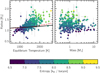 |
Fig. 1 Equilibrium temperature–radius diagram (left panel) and mass–radius diagram (right panel) color-coded by entropy for the 314 hot Jupiters selected for our analysis. The solid black and the red dashed lines compare the radii computed using our model completo21 and TF18, respectively. Both models are for a 1 MJ planet with a pure H/He composition with Y = 0.27 at 5 Gyr and without accounting for inflation. The entropy was computed using the observed physical properties and an assumedheavy-element fraction of 0.2. Planets with large radii tend to have high internal entropy, with a weak dependence on planetary mass. |
3 Interior structure model
The primary way to gain insights into the interior structure of exoplanets is typically derived from theoretical structure models by matching the observed mass and radius. Such models are often used to constrain the planet bulk composition. Given the age of the host star and the mass of the planet, the amount of heavy elements is determined by matching the observed radius with the radius predicted from structure models. This has been applied to warm Jupiters (e.g., Thorngren et al. 2016), sub-Neptunes (e.g., Valencia et al. 2013), and super-Earths (e.g., Dorn et al. 2019) but is challenging to apply for hot Jupiters because the radii are inflated.
The aim of our study is to characterize the interior structure of hot Jupiters within a probabilistic framework. This allows us to gain insights into the physical properties governing the interior. We are specifically interested in inferring the internal luminosity of the planets based on the observed mass, radius, and equilibrium temperature. This in turn will provide constraints on the heating efficiency, internal temperature, and the pressure at the radiative–convective–boundary (RCB). The standard interior structure model is briefly outlined in Sect. 3.1 and we discuss in Sect. 3.3 our approach to account for heat dissipation. The main model assumptions and limitations are addressed in Sect. 3.4.
3.1 Standard model
The planetary evolution model completo21 was presented in Mordasini et al. (2012) and several modifications have been introduced since such as photoevaportation (Jin et al. 2014; Jin & Mordasini 2018) and coupling the interior to a nongray atmospheric model (Linder et al. 2019; Marleau et al. 2019). In the following sections, we provide a brief description of the code relevant to our work and discuss in Sect. 3.4 the limitations of the model.
The internal structure of a gas giant planet is modeled using the 1D equations below. Equation (2) defines the conservation of mass. We assume that the planet is in hydrostatic equilibrium (Eq. (3)) and that the luminosity is constant with radius (Eq. (4)). Mordasini et al. (2012) showed that the latter assumption does not significantly affect the evolution of the planet when the heating occurs deep, as we assume (see below). Finally, Eq. (5) is the energy transport equation, describing the transport of energy either via radiation or convection:

In the above equations, r is the planetary radius as measured from the center, m the total mass inside r, ρ density, P pressure, T temperature, l planet internal luminosity, G the gravitational constant, and ∇ is the temperature gradient which depends on the process energy is transported.
We use the classical SCvH EOS of hydrogen and helium (Saumon et al. 1995) with a He mass fraction Y = 0.27. Our model does not include a central core and all the heavy elements are homogeneously mixed in the gaseous envelope, see Sect. 3.4.1 for a discussion on the distribution of heavy elements. We model the heavy elements as water and adopt the widely used EOS of water ANEOS (Thompson 1990; Mordasini 2020). H/He and water are mixed according to the additive volume law (Baraffe et al. 2008). The transit radius is defined at P = 20 mbar.
3.2 Atmospheric model
The atmospheric boundary conditions control the cooling rate of irradiated giant planets. The evolution of the planet and its final structure are thus sensitive to the upper boundary conditions (Guillot & Showman 2002). Jin et al. (2014) calibrated the semi-gray model of Guillot (2010) against the fully nongray atmospheric models of Fortney et al. (2008) in order to determine the value of γ, the ratio of the optical to the infrared opacity. They used a nominal value of Tint = 200 K. For our study, hot Jupiters are thought to be inflated due to dissipation or advection of heat into the interior, which thus leads to Tint > 200 K. Hence, using the tabulated values of Jin et al. (2014) will lead to different PT structures and therefore alter significantly the interior structure of the planet. Indeed, we find that for Teq = 1500 K, Tint = 500 K, and log g = 3, the relative change in the radius between using the improved version of the semi-gray model and using a nongray model is around ~ 7%, where the semi-gray model tend to lead to larger radii. It is essential then to have realistic atmospheric boundary conditions by using wavelength dependent radiative transfer atmospheric models.
Following a similar approach to Linder et al. (2019), we compute a grid of fully nongray atmospheric models calculated using the petitCODE (Mollière et al. 2015, 2017). We included the following line absorbers CH4, H2 O, CO2, HCN, CO, H2, H2 S, NH3, OH, C2 H2, PH3, Na, K, TiO, VO, and SiO, and the following pseudo-continuum absorbers H2 -H2 Collision Induced Absorption, H2-He Collision Induced Absorption, H− bound-free, H− free-free, H2 Rayleigh scattering, and He Rayleigh scattering. The reference for these opacities can be found in Mollière et al. (2019). These grids are then used to relate the planet atmospheric temperature and pressure to the planet internal structure. The atmospheric grid was calculated assuming solar composition and covering a range of 2.5–4.5 in log g, 500–2700 K in equilibrium temperature, and 100–1000 K in internal temperature. The equilibrium temperature and surface gravity were chosen to cover the range of all the hot Jupiters selected in our sample.
The coupling between the atmosphere and the interior is done in the interior adiabat, following the first convective layer below the RCB. Details are given in Marleau et al. (2019). For a given log g, equilibrium temperature, and internal temperature, the corresponding pressure and temperature were used as boundary conditions to calculate the inward interior structure. The outward structure was calculated using the petitCODE structure and assuming hydrostatic equilibrium (Eq. (3)) between the pressure at the coupling point and 20 mbar, that is, the pressure at which the transit radius is defined. We verify that coupling at a high fixed pressure, P = 1000 bar, or following the RCB layer does not significantly affect the transit radius with relative change around ~ 0.3%.
The atmospheric PT structures assume constant log g. In fact, log g changes slightly in the radiative layers. Assuming that the change in log g in the radiative layers during the planet evolution is around ~ 0.05, then the change in entropy is only around ~0.05 kB/baryon for an internal temperature(Tint) of 700 K and an equilibrium temperature(Teq) of 2500 K. It would take a change of 0.5 in log g to have a significant change in entropy (around 0.5 kB baryon−1 for Tint = 700 K and Teq = 2500 K). We confirm that the change in entropy is negligible across the entire grid except for models with Teq > 2500 K, Tint > 700 K, and log g < 3.5. In our sample, only WASP-12 b has Teq = 2580 K and log g = 3.0 (Collins et al. 2017) where the change in entropy is between 0.06 and 0.08 kB baryon−1. The radius of only one planet in our sample could be slightly underestimated, and therefore a constant log g in the PT structures is not a strong assumption.
3.3 Heat dissipation
It is well established that, compared to cold Jupiter-like planets, the high internal entropy of a hot Jupiter increases its radius (Spiegel & Burrows 2013; Marleau & Cumming 2014). For example, the planet interior can gain entropy through ohmic or tidal heating. In this work, we do not attempt to model a mechanism to transport heat into the interior. We assume the planet is in steady state and thus do not calculate the planetary thermal evolution. We use the planet mass, radius, and equilibrium temperature (technically the stellar luminosity and the semimajor axis) from observations along with the mass–heavy-element-mass relation from Thorngren et al. (2016), to quantify the present internal luminosity Lint of the planet. At steady state, Lint is identical to the extra heating power deposited and thus

where ϵ is the fraction of stellar irradiation transported into the interior, that is, the heating efficiency, σ is the Stefan-Boltzmann constant, Rp the planetary radius, and F is the flux the planet receives at the substellar point as a function of the stellar temperature T*, stellar radius R*, and the semi-major axis a (Guillot 2010). We assume that the heat dissipated is absorbed at τ = 2∕3 and deposited at the center of the planet. Komacek & Youdin (2017) showed that heating at any depths larger than 104 bar yields nearly similar radii. However see the discussion relevant to this assumption in Sect. 3.4.2. Our definition agrees well with TF18, where they also deposit the extra heat at the center.
We notethat 1D models without extra heating do not transfer energy into the interior on their own. The main effect of irradiation is that it decreases the cooling rate and thus the contraction rate of irradiated giant planets (Burrows et al. 2000). Planets with higher Teq will have a larger radius compared to an identical planet with lower Teq but still, not as large as the observed radii. The black line in Fig. 1 shows the radius for a 1 MJ planet with a pure H/He envelope at 5 Gyr at different Teq. All planets have Rp < 1.25 RJ. The difference in the radius between the highly and least irradiated planets is 0.14 RJ. As such, our definition of ϵ is valid where all the extra energy is transported into the interior via a physical mechanism and it is not due to the 1D irradiated models transporting energy at high Teq.
3.4 Model assumptions and limitations
3.4.1 Distribution of heavy elements
The distribution of heavy elements in the interior of exoplanets is still an open question. Some models assume for simplicity that all the heavy elements are in the core (Mordasini et al. 2012). For warm Jupiters, Thorngren et al. (2016) set an upper limit of 10 M⊕ of heavy elements in the core and the rest is mixed homogeneously in the envelope. Current models developed to explain the anomalously large radii of hot Jupiters mix all the heavy elements in the envelope and do not include a central core (e.g., TF18; Komacek & Youdin 2017).
From the Juno mission, we now know that Jupiter has a diluted core (Wahl et al. 2017) based on the measurements of Jupiter’s low-order gravitational moments (Folkner et al. 2017), yet these findings are challenging to explain from standard formation models (Muller et al. 2020). Even though the interior structures are highly affected by the chosen equation of state, the prediction of an enriched envelope still holds (Wahl et al. 2017). Planet formation models based on core accretion and that include the effect of envelope enrichment, also suggest that gas giant planets can be formed, notably at an accelerated rate (Venturini et al. 2016). Envelope enrichment compared to the Sun has also been observed for all of our four giant planets (Guillot & Gautier 2014).
In this work, all the heavy elements are mixed homogeneously in the convective part of the interior and are made up entirely of water. A central core is therefore not included. We compare the effect of the distribution of the heavy elements in the core versus in the envelope on the transit radius of the planet and hence on the heating efficiency ϵ. We find that for HD 209458 b, 42 M⊕ distributed in the core or in the envelope do not change significantly the radius when we account for heating in the interior. The absolute relative change in the radius is less than 2% for ϵ ranging 0− 5%. These results are also in agreement with Thorngren et al. (2016), which reached the same conclusion without accounting for heat dissipation. The median relative uncertainties on the radii measurements from observations in our sample is 4.3%, thus the distribution of the heavy elements has little effect on the inference of Lint and therefore ϵ. We also show in Sect. 6 that the uncertainty on the heating efficiency is mainly dominated by the amount of heavy elements in the planet rather than their distribution within the planet.
3.4.2 Depth of internal heating
In our model, we assume that the heat is deposited in the interior of the planet. However, the pressures at which heat is deposited is still not constrained. Within the context of ohmic dissipation (Batygin & Stevenson 2010), the depth of internal heating is mainly dominated by the electrical conductivity profile and by the depth of the wind zone. The layers that contribute the most are the layers close to the RCB. At lower pressures heat is reradiated, whereas at higher pressures ohmic heating is not efficient due to the high conductivity there (Batygin & Stevenson 2010; Batygin et al. 2011). Huang & Cumming (2012) deposit the extra heat in the radiative layers and do not include ohmic heating below pressures of 10 bar. Under these assumptions, the RCB moves to higher pressures. Wu & Lithwick (2013) showed that heat deposited at deep layers requires significantly less heating efficiency in comparison to depositing the extra heat at shallow pressures. For planetary parameters similar to TrEs-4 b and using the same heating efficiency, the model of Batygin & Stevenson (2010) yields a planetary radius of 1.9 RJ, while under a similar model Wu & Lithwick (2013) yields 1.6 RJ. Differences in the radial profiles of the conductivity and wind might explain this difference. This however shows the difficulty in comparing models under the same heating mechanism but using different assumptions.
Komacek & Youdin (2017) studied systematically the effect of varying the depth of heating on the radius and found that heat deposited in the convective layers can explain the radii of hot Jupiters. Modest heating at pressures larger than 100 bar is enough, on condition that the heating is applied at an early age while the interior at such pressures is still convective. Heating at any pressure deeper than 104 bar leads to similar radii.
All the results we show are based on the assumption that heat is deposited in the deep interior. Therefore, the heating efficiencies we compute could be underestimated. This potentially has also an effect on the interior structure of hot Jupiters, where we show that the RCB moves to lower pressures.
4 Statistical model
Our goal is to estimate the internal luminosity and heating efficiency for the individual planets and for the population of hot Jupiters, while accounting for the uncertainties on the observed parameters. In this section, we describe the method used to infer the distribution of the internal luminosity and thus the heating efficiency for each planet, by establishing a probabilistic framework to link the observed planetary radius to the predicted one from the theoretical model described in Sect. 3. We start by describing how the internal luminosity for each individual planet is computed in Sect. 4.1. We refer to this step as the lower level of the hierarchical model. In Sect. 4.2, we then combine the individual posterior samplings to study the global distribution of the full population. This will be referred to as the upper level of the hierarchical model.
4.1 Lower level of the hierarchical model: inferring Lint for each planet
For each planet n (n = 1, 2, …, N), the planetary radius Rp,n depends in our model on the planetary mass Mp,n, the fraction of heavy elements Zp,n, the planet internal luminosity Lint,n, and the stellar incident flux Fp,n, which further depends on the stellar luminosity L*,n and on the semi-major axis an. In what follows, all the quantities refer to the individual hot Jupiter’s physical parameters. In this framework, we define ωn, the parameters that determine the planetary radius for each individual hot Jupiter
 (8)
(8)
and thus the predicted radius from the theoretical models Rt,n is a deterministic function of ωn, where Rt,n = f(ωn). Rt,n is determined using the internal structure model described in Sect. 3. Given the observed planetary mass, semi-major axis, and stellar luminosity, and using the mass–heavy-element mass relation from Thorngren et al. (2016), we aim to infer the distribution of Lint,n that reproduces the observed radius. We thus intend to answer the question: what is the internal luminosity of the planet giventhe observable parameters and our assumption on the fraction of heavy elements? Therefore, we define the likelihood function, the probability to observe the data given a specific set of model parameters, as
 (9)
(9)
Finally, the posterior probability function, the probability of the parameters ωn given the data Dn, is

In the last line in Eq. (12) we assume that Lint,n, L*,n, and an are independent of each other and that Zp,n depends on Mp,n following the mass–heavy-element mass relation (Thorngren et al. 2016). This inference allows us to account for data uncertainties. The semi-major axis is known precisely from observations and hence we fix the value to the observed one. We then marginalize over Mp,n, Zp,n, and L*,n to infer the distribution of the internal luminosity. We assume that the distribution of each of the observed parameter is a Gaussian distribution centered on the true quantity with a scatter given by the measurement uncertainties. Following the standard statistical notation, we can write

where α, β, and σZ are the values taken from the mass–heavy-element mass relation established by Thorngren et al. (2016). We use α = 57.9∕317.828, β = 0.61, and σZ = 101.82∕317.828 where 1MJ = 317.828 M⊕ and Mp is in Jovian mass MJ. Here,  implies that y is drawn from a normal distribution
  with mean μ and standard deviation σ.
  denotes that ϵ is sampled from a uniform distribution. We perform the inference twice each time using a different prior for the internal luminosity

where we set τ0 = (a, b) = (0, 5).  and
and  implies that Lint is drawn froma log-uniform and uniform distribution, respectively, and Lint is in Jovian luminosity LJ. We note that in our analysis, we do not sample ϵ, we sample Lint and at each step in the Markov chain Monte Carlo (MCMC) compute ϵ using
 (19)
(19)
which was obtained by combining Eqs. (6) and (7) and the relation between the stellar luminosity and flux. We further set a uniform prior on ϵ over the range 0−5% (Eq. (17)).
In Eq. (18a), Lint,n is sampled from a log-uniform distribution  . We choose this prior because the internal luminosity covers a wide range of values and little is known about the true underlying distribution. This prior however does not lead to a uniform distribution in ϵ (see Sect. 4.1.1 and the right panel of Fig. 3 for details), we therefore also consider a prior distribution uniform in linear space (Eq. (18b)). The distribution of ϵ is uniform under this prior. In Sect. 4.1.1 we show in detail how the choice of prior on the internal luminosity affects the prior on ϵ and we discuss its effect on the inference. Finally, we can use the structure models to compute the internal temperature Tint. As discussed in Sect. 3.2, the atmospheric models were computed for Tint between 100 and 1000 K. We therefore setan upper limit of Tint < 1000 K in order to avoid extrapolation.
The statistical model described in Eqs. (13)–(18b) and setting Tint < 1000 K contain all the relevant distributions to evaluate Eq. (12). All the results shown in Sect. 6, were produced byrunning MCMC using emcee (Foreman-Mackey et al. 2013). For each planet, we ran MCMC with 50 walkers each with 1000 steps and discard the first half as burn-in. At each iteration we compute the heating efficiency ϵ using Eq. (19). Using 25 000 samples we then marginalize over the nuisance parameters and infer the posterior distribution of Lint,n and of ϵ. The average acceptance ratio was around ~0.5 for almost all the planets in the sample.
As a by-product of this analysis, we also keep track of the PT profiles and thus infer the distribution of the pressure at the RCB and the planet internal temperature Tint. This is useful to gain insights on the interior structure of hot Jupiters and we present the analysis in Sect. 6.4.
4.1.1 Choice of prior on the internal luminosity
In the lower level of the hierarchical model (Sect. 4.1), we use noninformative uniform distributions in log and linear space as prior for the internal luminosity. It is worth studying the effect of the prior distribution on the final results. Figure 2 shows the marginalized distributions for HD 209458 b using the two different priors. The luminosity distribution is shown in log-scale for both distributions for illustrative purposes. Red shows the samples using a log-uniform distribution while blue using a uniform distribution in linear space. Note the strong correlation between the fraction of heavy elements Zp and the internal luminosity with a Pearson correlation coefficient ρ > 0.9. The observed parameters (Rp, Mp, and L*) are reproduced in both cases and the distributions look almost identical. But the distributions of Lint, the main parameter of interest, are different leading thus to different distributions in heating efficiency ϵ. We are in a regime where the data size is small and the choice of the prior distribution is important and dominates the inference. We note that Fig. 2 shows the radius distribution even though we do not sample this parameter. This is useful to validate the model and to check that it predicts the observed data. Such plots are referred to as posterior predictive plots and we apply them in Sect. 6.1 to validate the model for each planet.
Ideally, we would want to learn about the internal luminosity of the planet by relying entirely on the observed parameters while the choice of the prior should have minor effects on the posterior inference. Even though both distributions are noninformative, the data is not enough that the prior dominates. To put it in another way, more data is needed to be able to infer the distribution of Lint independently of the choice of prior. Unfortunately, the physical parameters that can be observed for exoplanets in general and transiting planets specifically are very limited. One promising avenue might be inferring precisely the internal temperature, which was for the first time recently estimated for WASP-121 b (Sing et al. 2019) with Tint = 500 K. In our results for WASP-121 b, the Tint distributions look similar using both priors and therefore it is not possible to put tighter constraints on Lint. Another promising approach is to put tighter constraints on the planet mass–heavy-element mass relation, which translates to tighter constraints on Lint due to the large degeneracy between Lint and Zp. This can be achieved by increasing the number of confirmed transiting warm Jupiters, that is, giant planets with Teq < 1000 K. Such relatively cool planets are not inflated (Demory & Seager 2011). This allows to infer the fraction of heavy elements for such planets and recalibrate the relation between the planet mass and fraction of heavy elements, similar to what was done by Thorngren et al. (2016) but with a larger sample.
It is important to explicitly mention that given the setup of the statistical model, the prior distributions for the individual planets are not the same because of the imposed upper limit of ϵ = 5%, which further depends on the observed parameters (Eq. (19)). This can be understood by looking at the bottom line in Eq. (12)3, where it is clear that each planet has different L*, Mp, a, and Zp distributions due to differences in the observed physical properties. We confirm this by sampling the prior probability density function (PDF), that is, by running the model on an empty data set Dn for two different planets EPIC-211 418 729 b and WASP-48 b. By not sampling Dn in Eq. (12), we effectively sample the prior PDF. The left panel of Fig. 3 illustrates this concept where we show that the internal luminosity prior distributions are different under the linear-uniform prior for both planets. Note though the log scale for better visualization. Even though we imposed a uniform distribution between 100 and 105 LJ, Lint larger than 102.5 LJ for EPIC-211418729 b are not sampled and thus are ruled out. This cutoff in the distribution at high Lint values is a consequence of the upper limit imposed on ϵ and the low stellar luminosity which translates to low Teq. With an equilibrium temperature roughly of Teq = 700 K, a heating efficiency of 5% for EPIC-211 418 729 b is equivalent to a maximum Lint = 102.5 LJ. On the other hand, WASP-48 b with Teq = 2000 K (i.e., high L*), an upper limit of 5% on the heating efficiency is equivalent to a maximum of Lint ~ 105 LJ. We note that for WASP-48 b low Lint values are not ruled out but are less probable. To summarize, even if the initial prior imposed on Lint is  with a = 0 and b = 5, the actual prior distributions for the individual planets are different with different a and b values. This is a consequence of the additional prior on ϵ (ϵ < 5%). Planets with low Teq, their distributions are truncated at high Lint values (with b < 5). While this is not the case for planets with high Teq (with b = 5). The importance of a and b is relevant for the discussion in Sect. 4.2.
It is also worth studying the consequence of using different Lint priors ( and
and  ) on the heating efficiency ϵ prior PDF since the relationship between the two parameters is deterministic following Eq. (19). We follow the same procedure described in the previous paragraph, that is, we run the model on an empty data set for EPIC-211418729 b. The right panel of Fig. 3 shows samples from the prior distribution on ϵ for EPIC-211418729 b using the linear-uniform and log-uniform cases. It is evident that a log-uniform prior distribution on Lint does not lead to a uniform prior on ϵ and the inference is biased toward small ϵ values. Whereas this is not the case when assuming a linear-uniform prior on Lint. We want to stress that this holds for almost all of the planets in our sample and not only for EPIC-211418729 b, which was chosen arbitrarily.
From a statistical point of view, a log-uniform prior distribution is favored because of the large range of values and it is therefore easier to explore the entire parameter space in log space. However, this prior leads to biases in the ϵ distribution. To mitigate this, in the following section (Sect. 4.2) we develop a flexible hierarchical Bayesian model that accounts for the choice of prior. We study the population distributions under both priors in Sect. 6 and show that the inference at the population level is independent on the choice of prior.
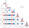 |
Fig. 2 Posterior distributions inferred for HD 209458 b using our model (Eq. (12)). The gray dashed lines show the observed value for the relevant parameters. The effect of using different prior distribution leads to different posterior distributions for Lint, ϵ, and Zp. The inferred posterior distributions for the other parameters (L*, Mp, and Rp) are almost identical for both priors since they are constrained well from observations. |
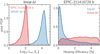 |
Fig. 3 Left: PDF of the prior on the internal luminosity distributions for WASP-48 b and EPIC-211418728 b under the linear- |

4.2 Upper level of the hierarchical model: population level posterior samplings
4.2.1 General framework
In Sect. 4.1, we inferred the distributions of Lint, ϵ, Tint, and pressure at the RCB (PRCB) for each planet individually. In this section, we derive the equations needed to study the general distribution of the (i) internal luminosity as a function of planet radius, (ii) heating efficiency, (iii) internal temperature, and (iv) pressure at the RCB as a function of Teq. The distributions (i), (iii), and (iv) provide insights into the interior structure of hot Jupiters while (ii) gives insights into the efficiency of transporting energy into the interior, similar to the work of TF18.
Distributions (i) and (iv) are modeled using a 4th degree polynomial
 (20)
(20)
The set of parameters describing the population is referred to as hyperparameter and defined as  . x is the planet radius Rp for (i) and equilibrium temperature Teq for (iv). There are many benefits of using polynomial regression compared to other parametric and nonparametric approaches. One important factor is that these models are flexible and can take a variety of shapes and curvatures to fit the data, making the results thus less model dependent compared to parametric models. Another important factor is that polynomial regression is similar to fitting a linear model and thus is computationally inexpensive and very fast to compute, unlike nonparametric models such as Gaussian process. A disadvantage to this approach is the curse of dimensionality, where the number of model parameters grows much faster than linearly with the growth of degree of the polynomial. In our case, weuse univariate polynomial regression with degree 4 and thus the total number of model parameters is 5.
Distribution (ii) is modeled using both a 4th degree polynomial and a Gaussian function
![Mathematical equation: \begin{align*} g_g \left({T_{\textrm{eq}}} \right)\,{=}\,{\epsilon_{\textrm{max}}} \exp \left[ -\frac{1}{2}\left(\frac{{T_{\textrm{eq}}}-{T_{\textrm{eq}}}{_0}}{s} \right) ^2 \right]\end{align*}](/articles/aa/full_html/2021/01/aa38361-20/aa38361-20-eq21.png) (21)
(21)
where the hyperparameters 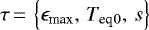 are the amplitude, the temperature at ϵmax, and the width of the Gaussian function, respectively.
Finally, distribution (iii) is modeled using a Gaussian function with the hyperparameter 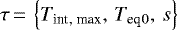 .
.
4.2.2 Derivation
In what follows, we derive the key equation which the inference is based on (Eq. (28)) but first provide the motivation and simple description of the method. We aim to use the single distributions we inferred in the lower level of the hierarchical model to infer the set of population parameters τ, which we refer to as hyperparameters. The general form of the full posterior distribution in the hierarchical framework is
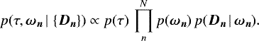 (22)
(22)
In this equation N is the total number of planets, p(τ) is the prior probability distribution on the hyperparameters, p(ωn) and p(Dn | ωn) are the prior and likelihood distributions for the individual planets, respectively. The population posterior distribution is a strong function of the prior imposed at the lower level of the hierarchical model. This can be understood if we assume that p(ωn) is the same for all planets. Using this assumption,  scales with
  .
.
It is crucial therefore to make sure that the distribution we infer for the population has physical origins rather than is an output of the choice of prior. Hence, in order to account for the prior distribution imposed at the lower level of the hierarchical model, we apply the importance sampling algorithm. We follow closely the pioneering work established by Hogg et al. (2010) (see also the Appendix of Price-Whelan et al. 2018). This method has been used by Foreman-Mackey et al. (2014) to infer the occurrence rate of planets as a function of period and radius and by Rogers (2015) to infer the radius at which the composition transition from rocky super-Earth to volatile-rich sub-Neptunes. Briefly, we reweight the individual posterior samples by the ratio of the value of the hyperparameters τ evaluated given the new hyperprior distribution to the old prior on which the individual sampling is based on evaluated at the old default τ0 values. We derive below the marginal likelihood distribution.
For each n of N planets, we obtain K posterior samples of the parameters that determine the planetary radius θn = (Mp,n, Zp,n, L*,n, an) and Lint,n. Following similar notation to Sect. 4.1 and for brevity, we define the full set of parameters as
 (23)
(23)
We use the individual posterior samplings to compute the likelihood of the hierarchical model. For a single planet, the likelihood given the hyperparamters τ is

where in the last equation we applied Bayes’ theorem on the posterior distribution p(ωn | Dn, τ0), which is the posterior distribution for a single planet computed using Eq. (12). The set of parameters from which the previous inference was generated is denoted by τ0. For example, as described in the previous section, the parameters describing the distribution of Lint are τ0 = (a, b) = (0, 5). We can then apply the Monte Carlo integral approximation to estimate the marginalized likelihood distribution over θ
 (27)
(27)
Essentially, we are assuming that all the probability integrals can be approximated as sums over samples. In case of infinite samples, this approximation becomes exact. Having derived the marginalized likelihood distribution for a single planet (Eq. (27)), the full marginal likelihood is then the product of the individual likelihoods
 (28)
(28)
We can then choose a prior probability distributions for the hyperparameter τ and the posterior probability distribution is
![Mathematical equation: \begin{align*} p(\tau \, | \, \left\lbrace {\bm{D_n}} \right\rbrace) &\propto p(\tau) \, \prod_{n}^{N} p({\bm{D_n}} \, | \, \tau) \\[4pt] &\approx p(\tau) \, \prod_{n}^{N} \frac{1}{K} \sum_k^K \frac{p(y_{nk} \, | \, \tau)}{p(y_{nk} \, | \, \tau_0)}.\end{align*}](/articles/aa/full_html/2021/01/aa38361-20/aa38361-20-eq31.png)
Inside the sum, the numerator is the new probability distribution that we want to infer given a new set of hyperparameters τ, while the denominator is the value of the default prior on which the single posterior samples is based at the previously assumed values of τ0. We then reweight theynk posterior samples by the ratio. This approach of using the posterior samples from the lower level of the hierarchical model like data in the upper level has been first addressed by Hogg et al. (2010) (see also Foreman-Mackey et al. 2014, and TF18). Ideally, the inference of τ and ωn for all the planets should be done simultaneously, however this is computationally very expensive as it involves solving 4N + m integrals, where N is the number of planets and m is the number of hyperparameters in our model.
Equation (28) is the main equation we use to infer the general distributions of (i), (ii), (iii), and (iv) defined at the beginning of this Section. We use Kernel Density Estimation (KDE) to estimate the probability density function (PDF) of each of the previously inferred distributions to compute p(ynk | τ), where we discuss below the functional forms. We note that even though we define a flat distribution for the internal luminosity, Eqs. (18a) and (18b), and set τ0 = (a, b) = (0, 5), this is not strictly the case because additionally we truncate the heating efficiency 0 < ϵ < 5% and require 100 < Tint < 1000 K. Also, as noted in Sect. 4.1.1, each planet has a different prior probability distribution, leading thus to different values of τ0 for each planet (for an example see left panel of Fig. 3). Therefore to evaluate p(ynk | τ0), we sample Eq. (12) for each planet on an empty data set similar to what was done in Sect. 4.1.1 and then estimate the PDF using KDE.
For each of the four distributions, we define the general form ynk = g(xnk), specifically ynk =

where Rp, nk and Teq, nk are the samples of the individual posterior distributions for the planetary radius and equilibrium temperature, respectively. The latter was computed at each iteration in the MCMC at the lower level of the hierarchical model and the values were stored.
4.2.3 Computational details
We summarize below the computational procedure. First, at each iteration in the MCMC we sample the hyperparameters τ and evaluate the function ynk = g(xnk) using the sampled values of τ. Second, we compute p(ynk | τ) and p(ynk | τ0) using the precomputed KDE functions. Finally, we evaluate the log-likelihood of Eq. (28)
![Mathematical equation: \begin{align} \textrm{ln} p(\left\lbrace {\bm{D_n}} \right\rbrace \, | \, \tau) &\approx \sum_n^N \left[ \textrm{ln} \left(\sum_k^K \frac{p(y_{nk} \, | \, \tau)}{p(y_{nk} \, | \, \tau_0)} \right) - \textrm{ln} K \right]\\ &\approx \!\sum_n^N \!\left[ \textrm{ln} \left(\!\sum_k^K\! \exp \left(\textrm{ln} p(y_{nk} \, | \, \tau) - \textrm{ln} p(y_{nk} \, | \, \tau_0) \right) \!\right) - \textrm{ln} K \right]\end{align}](/articles/aa/full_html/2021/01/aa38361-20/aa38361-20-eq33.png)
where in the last equation we compute the log of the sum of exponentials (log-sum-exp). In practice, this is numerically more stable compared to evaluating Eq. (35).
For all the results presented below, we use emcee to sample from the posterior probability distribution (Eq. (30)). The functional forms of g(xnk) are either a 4th degree polynomial or a Gaussian function or both. These are specified in Sect. 6. In what follows, we draw K = 2000 random samples from the single posterior samples when evaluating the mass–luminosity–radius relation. For the other relations we set K = 1 and use the observed Teq values. This is possible since the equilibrium temperature is often well constrained from observations. We verified that accounting for the uncertainties does not effect the results. We adopt 44 walkers and run the sampler for 4000 iterations where the first half are discarded as burn-in and retain only every 20th sample in the chain to produce independent samples. We monitored convergence by computing the acceptance ratio and by visually inspecting the trace plots and corner plots. We note that for each relation, we execute this procedure twice, each time using the samples drawn under the different prior, log-uniform  and uniform
  . By running this process twice, in Sects. 5 and 6 we show that the results are not biased by the choice of prior, unlike the lower level of the hierarchical model. All the data and results are available online4 and the source code can be found on github5.
5 Model validation using planet population synthesis
To validate the statistical method, we applied the hierarchical model to a synthetic catalog based on planet population synthesis. The true distribution under which the synthetic dataset was generated is known. Applying thus our hierarchical model on this dataset allows us to evaluate the quality of the fit and to check whether the statistical model gives an accurate representation of the real distribution based on the observed data.
5.1 Generating synthetic catalog
The data set was generated using the Generation III Bern model of planetary formation and evolution (Emsenhuber et al. 2020). Inflation was accounted for by including a parameterized bloating model with a small addition during the formation phase compared to Eq. (6) defined as
 (37)
(37)
where τmp is the optical depth in the disk midplane from the star to the planet. This relation takes into account that at early times the disk is optically thick and the planet is at large semimajor axis, therefore bloating is inefficient. At later times, the planet migrates inward, the disk dissipates, and the heating becomes relevant. Mol Lous & Miguel (2020) showed that migration can affect the inflation and radius of the planet only when high fraction of energy is deposited into the interior (ϵ > 5%) but has no effect for smaller ϵ values.
For the heating efficiency ϵ, we use the Gaussian relation (Eq. (21)). Specifically, we use the values we infer using the log- and presented in Table 1. For more details check Sect. 6.3. Our model also assumes the heating efficiency is constant in time and the stellar mass was fixed to 1 M⊙. Using the same assumptions discussed in Sect. 3, the heavy elements are distributed homogeneously in the envelope and we use the fully nongray atmospheric models of the petitCODE.
We perform the same cut on the synthetic data, that is, we select only planets with 0.37 < Mp < 13 MJ and semi-major axis a < 0.1 au. Since the population synthesis did not produce hot Jupiters with Teq > 2250 K, we manually moved the planets inward by 0.04 au after the formation epoch. This however does not have an effect on the inference. The population synthesis consists of 30 000 single embryo per disk systems (population NG73) out of which 174 hot Jupiters made it into the synthetic sample.
One of the main advantages of the statistical model is the ability to account for uncertainties on the parameters. We generate synthetic uncertainties by calculating the relative uncertainty for Mp, Rp, T*, and R* based on the observed data and then taking the median of the computed values. The median of the relative uncertainty for Mp and Rp is 7 and 4%, respectively. Whereas the median of the relative uncertainty based on the observed data for T* and R* is 1 and 4%, respectively. These parameters were then used to calculate the uncertainty on L*.
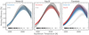 |
Fig. 4 Model validation on planet population synthesis data. Heating efficiency – equilibrium temperature (HEET) posterior distribution using the linear-uniform (left) and the log-uniform (middle) priors for a Gaussian and 4th degree polynomial. The thick lines denotes the posterior median for the relevant functions and the dashed black line denotesthe true distribution implemented in the Bern population synthesis model, which was used to generate the synthetic data. The dark and light shaded region contains the 68 and 90% credible interval. To better compare the same model using different priors, the right panel shows the Gaussian models using log (red) and linear (blue) uniform priors. The light gray model in the right panel is the inferred posterior distribution in case we do not correct for the choice of prior. Our model is able to retrieve the Gaussian-like function when modeled using a 4th degree polynomial. The posterior median provides a good fit to the true distribution although the linear model predicts a lower heating efficiency. The credible intervals derived are able to accurately constrain the true values of the model parameters. |
Comparison of the Gaussian function using the log and linear uniform prior along with comparison to TF18 results.
5.2 Performing statistical inference on the synthetic catalog
The Bern planet population synthesis model is based on the core-accretion model. As such, the model self-consistently computes the accretion of gas and solids onto the protoplanets, which we keep track of. We find that the mass of heavy elements is lower in the synthetic planets than inferred by Thorngren et al. (2016). We therefore refrain from using this relation in the lower level of the hierarchical model and replace Eq. (14) by
 (38)
(38)
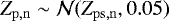
where Zps,n is the value from the population synthesis with a standard deviation of 0.05, which is equivalent to a relative uncertainty of 5%.
With this only modification to the original lower level of the hierarchical model described in Sect. 4.1, we apply the method to infer the distribution of Lint and ϵ for each of the synthetic planets. We compare the marginalized posterior distributions of the parameters to the simulated values and confirm that we were able to reproduce Mp, Rp, L*, and thus Teq for all the synthetic planets. We repeated this procedure twice each time assuming Lint follows a log-uniform  distribution or a linear-uniform
  distribution. The individual posterior distribution for most of the synthetic planets are flat, which highlights the need for a hierarchical model that combines the individual distributions to extract useful information at the population level. This is one of the main advantages of using hierarchical Bayesian model (Loredo & Hendry 2019).
We therefore use the marginalized ϵ distribution for each planet to infer the heating efficiency–equilibrium temperature (HEET) for the synthetic population following the method described in Sect. 4.2. We model the HEET distribution with both a Gaussian function and a 4th degree polynomial. The former function is used to test the ability of our hierarchical model to retrieve the input parameters of the Gaussian function and the latter function to test whether our model can indeed predict a Gaussian-like pattern.
5.3 Results using synthetic data
With this procedure, we end up with four posterior distributions, which are shown in Fig. 4. The left and middle panel show the inference done assuming Lint follows a linear-uniform and log-uniform distributions, respectively, for the Gaussian function and 4th degree polynomial. The right panel compares the Gaussian functions shown in the left and middle panel under both prior distributions. The black dashed line is the true distribution as implemented in the Bern population synthesis model. The dark and light shadedregion shows the 68 and 90% credible interval. The Gaussian-like pattern is retrieved when using a 4th degree polynomial and also in agreement with the inferred Gaussian distribution. The median posterior using the linear-uniform prior underestimates slightly the heating efficiency at the 68% (1σ) level but the true model is contained within the 90% (2σ) credible interval. This test shows that the statistical framework is able to retrieve the true distribution.
The light gray distribution in the right panel is the inference done assuming log-uniform distribution without correcting for the choice of prior at the lower level. This shows the importance of understanding the prior at the lower level and highlights the need to reweight the distributions.
6 Results using real data
We now apply the model described in Sect. 4.1, that is, the lower level of the hierarchical model, to infer the distribution of Lint, ϵ, Tint, and PRCB for each of the detected planets. In Sect. 6.1, we present diagnostic tools to validate the lower level of the hierarchical model. We then use the inferred posterior distributions to study the mass–luminosity–radius (MLR), Tint–Teq, PRCB–Teq, and heating efficiency – equilibrium temperature (HEET) distributions for the population of hot Jupiters following the model introduced in Sect. 4.2. In Sect. 6.2, we show that by properly correcting for the choice of prior, the MLR distribution at the population level is prior independent. We hence present the rest of the results under the uniform in linear space prior in Sects. 6.3–6.4. For completeness, we show the results using both priors in Appendix A.
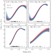 |
Fig. 5 Mass–luminosity–radius (MLR) posterior distribution for four different mass bins showing the median (thick line) and 68% credible interval (shaded area) assuming a uniform prior in log (blue) and linear (red) space. Using either prior leads to almost identical results. The internal luminosity is high with the largest planets having a luminosity approximately four orders of magnitude larger than Jupiter. |
6.1 Posterior predictive checks
For each system, we infer the distribution of the internal luminosity that reproduces the observed radius, mass, and stellar luminosity while fixing the semi-major axis to the observed value. We visually inspect each systemto double check that the marginalized posterior distributions of the observed parameters, Mp, Rp, L*, and thus Teq, are reproduced. Such plots are important to check that the model is a good fit and is thus capable of generating data that resemble the observed data. There are in total 17 systems where the observed mass and/or radius was not reproduced and thus we exclude these systems from the data set and do not include them in the analysis presented below. For most of the planets the radii are not possible from theoretical models as they are at the edge of the computed grid for a given planet mass, stellar luminosity, and semi-major axis. The observed radii tend to be larger than what is possible from the theoretical grid and most of these planets have masses Mp > 2.5 MJ. We note that for three systems the stellar luminosity and therefore the equilibrium temperature was not reproduced (HAT-P-20, Qatar-2, and WASP-43). We decide however to keep these systems since the difference in the equilibrium temperature is on the order of ~ 30 K and hence the change in the internal luminosity is almost insignificant.
6.2 Mass–Luminosity–Radius (MLR) distribution
We divide the samples into four mass ranges, similar to the mass bins estimated by Sestovic et al. (2018) but further divide their second mass bin into two: the sub-Jupiter planets (0.37−0.7 MJ and 0.7−0.98 MJ) and the massive-Jupiter planets (0.98−2.5 MJ and > 2.5 MJ). The number of planets in each group is 86, 59, 119, and 33 planets, respectively. To infer the MLR distribution, we run the model (Eq. (28) or equivalently Eq. (36)) for each mass bin by specifying the functional form of gp (x) as a 4th degree polynomial using Eq. (20). As such, x is the planet radius Rp in Eq. (20) and the hyperparameter  .
.
At each iteration in the MCMC, we compute ϵ following Eq. (19), where the semi-major axis is fixed to the observed value and L* and Rp are drawn from the individual marginalized posterior distributions. We further impose an additional log-normal prior on  for the planets with an equilibrium temperature less than 1000 K. This reflects our beliefs that planets with low equilibrium temperatures are not inflated (Demory & Seager 2011), and thus ϵ should be small. We tested several prior probability distributions on ϵ and verify that our results are not affected by the choice prior. We repeat the full procedure twice each time drawing samples from the lower level of the hierarchical model under the different priors at the lower level (
 and
and  ) and assign uniform uninformative priors on the hyperparameters. In Tables A.1 and A.2 we give the 68% credible interval values assuming linear-uniform and log-uniform priors and provide the chains online6.
Figure 5 shows the posterior distribution inferred for all mass bins under the two priors, uniform in log (red) and linear (blue) space. Notice that the lower right panel has a different scale to better visualize the results. Each data point is represented by a small line at the bottom of the plot at the corresponding radius. Such plots are called rug plots and are used to visualize thedistribution of the data. The posterior distributions under both priors are almost identical and indistinguishable inline with the conclusion reached in Sect. 5 by validating the hierarchical model on synthetic data. There are few differences between both models, such as at small radii for the least massive planets and at large radii for the most massive ones. These differences are mainly dominated by the small number of planets in these regions. This highlights the importance of reweighting the samples by dividing by the prior used to do the sampling at the lower level of the hierarchical model. For the rest of the paper, we show the results under the prior uniform in linear space, but confirm that the choice of prior at the lower level of the hierarchical model does not affect the main results and conclusions.
The basic shape of the MLR relation is similar across all mass bins, where as expected larger planets have higher internal luminosity with a plateau around 1.6 RJ beyond which the luminosity is almost constant. The small drop toward high radii has little statistical significance and likely reflects the choice of a fourth-order polynomial. The inferred internal luminosity for most of the planets is several orders of magnitude larger than Jupiter, reaching even up to four orders of magnitude. We also find that the internal luminosity is mass dependent, with the most massive planets having the highest internal luminosity.
A noticeable feature is that the sub-Jupiter planets with masses 0.37−0.98 MJ and radii less than 1 RJ have an internal luminosity larger than Jupiter. At first glance, one might expect such planets to have an internal luminosity smaller than Jupiter’s. We note however that the planets that have an equilibrium temperature less than 1000 K, indeed tend to have Lint ~ 3 LJ and not more. A higher luminosity is expected because, even with Teq < 1000 K, these planets are still much closer than Jupiter, which reduces the cooling rate and thus leads to higher internal luminosity. As for the planets that have equilibrium temperature larger than 1000 K, they tend to have higher fraction of heavy elements distributed in the envelope. There are only two sub-Jupiter planets in our sample that have radii less than 0.7 RJ, K2-60 and WASP-86, both of which require large fraction of heavy elements, 0.64 and 0.8, respectively, ruling out values less than 0.5. The high fraction of heavy elements explains the high luminosity values and the small number of planets with radii less than 1 RJ is why the distribution is poorly constrained in this regime.
6.3 Heating efficiency equilibrium temperature (HEET) distribution
Similar to the previous section, we also apply the model defined in Sect. 4.2 to study the HEET relation using both function forms: gp a 4th degree polynomial (Eq. (20)) and gg a Gaussian function (Eq. (21)) with  . The former is a flexible function that allows us to constrain the general shape of the relation by relying entirely on the data as motivated in the previous section, while the latter allows us to compare our results to TF18 and to theoretical predictions. Following the same methodology applied to the MLR relation, we further impose for the gp model the
  prior on the heating efficiency for planets with equilibrium temperatures less than 1000 K. We note that the individual distributions are flat, similar to the distributions of the synthetic planets and useful information can only be extracted by combining the individual distributions.
In Table A.3 we give the 68% credible interval values assuming  and
and  priors using the polynomial model. The Gaussian models are shown in Table 1 and the MCMC chains are available online7. The true distribution that was used to generate the synthetic data in Sect. 5 are the values we obtained using the log-
 prior and shown in Table 1.
The leftpanel of Fig. 6 shows that the posterior distributions are similar under both functional forms, with the polynomial function leading slightly to higher efficiencies. Using an independent interior structure model and a larger sample focused on FGK main-sequence stars, our results are qualitatively consistent with TF18. We confirm the Gaussian pattern holds independentof the choice of prior (see Fig. A.1). This pattern was predicted by ohmic dissipation first based on simulations (e.g., Menou 2012) and then later supported by TF18. Our analysis provides further evidence of the Gaussian-like distribution.
6.3.1 Comparison to TF18
To compare our results to TF18, we report the median and the 68% credible interval of TF18 in Table 1. We also show the posterior distributions in the right panel of Fig. 6. The heating efficiency increases until a maximum is reached at  , beyond which the efficiency decreases. Our result regarding the maximum heating efficiency agrees well within 1σ with TF18, where we determine ϵmax ~ 2.50%, compared to ~ 2.37%. In our model, the peak occurs at ~1860 K, while TF18 estimate the transition at ~1566 K. This discrepancy can be attributed either to differences in the statistical framework or in the interior structure model. We will address both next.
While TF18 used a nonparametric Gaussian Process (GP) approach to model the HEET distribution, they found consistent results with the Gaussian function. In our study, instead of modeling the HEET distribution with a nonparametric GP model, we use a flexible 4th degree polynomial that we stress is very fast to compute8 and find consistent results with the Gaussian function. To test whether this discrepancy could be due to the statistical framework, we ran our statistical model using the individual distributions inferred by the analysis of TF18, which were shared with us. We note that using their data, there is no need to reweight the distributions. See Sect. 6.3.2 for a detailed explanation. We confirm we were able to recover their posterior distribution using both a Gaussian function and a 4th degree polynomial. There is a very good agreement at the 1σ level, except for Teq < 1000 K where the results are slightly different. The amplitudes are in agreement at the 1σ level even though we find tighter credible intervals at the 1σ level but very good agreement at 2σ. With this we conclude that the differences are not due to the statistical framework.
We now study the differences in the interior structure model by comparing the solid black and dashed red models in the left panel of Fig. 1 computed using our model completo21 and by TF189, respectively. Both of these models are for a 1 MJ planet with a pure H/He envelope without accounting for inflation. In our case the planets are 5 Gyr old. Using our structure model, Rp ranges between 1.12 and 1.22 RJ for Teq between 800 and 2500 K. In comparison, Rp is between 1.11 and 1.31 RJ using the TF18 models for the same Teq interval. While the radii at low Teq are almost identical, the differences at high Teq are up to ~0.1 RJ. We notice that both models lead to different radii starting at Teq > 1500 K. This difference could explain the higher heating efficiency we infer at Teq > 2000 K. Since the planets in our model have smaller radii starting at 1500 K, then more energy needs to be transported into the interior to reproduce the observed radius, leading to higher ϵ values compared to TF18. We note that this is a simple case scenario where the models are for planets made entirely of pure H/He. While this scenario explains the trend, more tests are needed to compare the radii at different Teq for different fraction of heavy elements since the details of the EOS for the heavy element could in principle also be a source of discrepancy between the models.
The discrepancy in the radii could be caused by differences in the atmospheric modeling. We next compare the atmospheric models of petitCODE and Fortney et al. (2007), which was used by TF18 and did not include TiOand VO. The previously computed atmospheric grid using petitCODE include TiO and VO (see Sect. 3.2). We therefore calculate the PT structure for a typical hot Jupiter at solar compostion, Tint = 100 K, Teq = 2000 K, and log g = 3.27 without accounting for these absorbers. We find that in the absence of TiO and VO no inversion was formed with similar profiles using both atmospheric models. We then calculate the entropy of both structures using our EOS. We find that the entropy in the convective layers at pressure of 104 bar is 7.55 kB baryon−1 using petitCODE compared to an entropy of < 7.65 kB baryon−1 at pressure of 1000 bar using the models of Fortney et al. (2007). We note that at this pressure the structure is still not convective and thus the entropy is smaller than 7.65 kB baryon−1 in the convective layers and most likely the difference is < 0.1 kB baryon−1 between both models. We note that when including TiO/VO the entropy is ~ 7.5 kB baryon−1. A higher entropy leads to larger radii (e.g., Spiegel & Burrows 2013; Marleau & Cumming 2014) and as such we conclude that the difference between both models presented in Fig. 1 could be due to differences in the opacities high up in the atmosphere, namely TiO/VO, which then have a larger effect on the deep atmosphere due to the (anti) greenhouse effect.
A more systematic comparison between both atmospheric models for different Teq and log g is required to further quantify the discrepancies, which is beyond the scope of this paper. We note that both studies do not account for systematic differences in the structure models. Such comparisons will therefore allow similar future studies to account for the systematic differences and thus infer more reliable credible intervals.
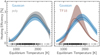 |
Fig. 6 Left: heating efficiency–equilibrium temperature (HEET) posterior distribution under the linear-uniform prior using a Gaussian function and a 4th degree polynomial. Right: the Gaussian function shown on the left side in comparison to the HEET posterior distribution inferred by TF18. The shaded region show the 68% credible interval. There is a good agreement between the Gaussian and poly models, which shows that indeed the HEET distribution follows a Gaussian function. Our results are in agreement with the findings of TF18 although the peak in our models is shifted to higher equilibrium temperatures. |
6.3.2 Are the results of TF18 prior dependent?
In short, no.
In our study, we sample Lint and then compute ϵ using Eq. (19). We imposed two different prior distributions on Lint because we do not have a priori knowledge which distribution best represent the population. Within a statistical framework, a log-uniform distribution is preferred in order to explore the entire parameter space. However, as we showed in the right panel of Fig. 3, this leads to biases giving more weight to lower heating efficiency. Whereas, a linear-uniform prior distribution on Lint leads to approximately a uniform prior distribution on ϵ.
As discussed in Sect. 4.2.2, the choice of prior distribution is important as the posterior distribution scales to the number of planets N. Thus the need to reweight the distributions at the upper level. Another way to approach this study is to perform a full hierarchical Bayesian modeling where the inference on both the individual planets and population is made simultaneously (Wolfgang & Lopez 2015; Wolfgang et al. 2016).
In the study of TF18, the setup is different. They sample ϵ and impose a uniform prior between 0 and 5%. There are no additional conditions that truncate the ϵ distribution, which itself is flat noninformative prior. Therefore, there is no need to reweight the distributions.
In general, it is always a good practice to sample the prior PDF distribution (Hogg & Foreman-Mackey 2018). This step is important to check whether MCMC samples correctly the specified prior distributions.
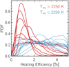 |
Fig. 7 Posterior distributions of the heating efficiency ϵ for all the planets with Teq > 2000 K. The colors indicate planets with Teq < 2250 K and Teq > 2250 K in blue and red, respectively. Six out of the seven planets shown in red favor small heating efficiency values with the most probable value close to ϵ ~ 1%. This provides evidence that the interior structure model disfavor high ϵ values and thus the decrease seen in the HEET distribution is real given our structure model. |
6.3.3 Thedecrease in efficiency at high Teq is real
In order to check whether the decrease in the heating efficiency at high Teq is real or not, we reran the lower-level model for all the planets with Teq > 2000 K. We assumed a linear-uniform prior for Lint to ensure the results are not biased toward small ϵ values. Additionally, we did not put constraints on Tint. This is important for the highly irradiated planets where Tint ~ 1000 K translates toϵ < 5%.
The main goal of this exercise is to check whether the interior structure model allows for high ϵ values for all the planets withTeq > 2000 K. The cutoff was chosen to be close to the peak of the Gaussian function as inferred previously in Sect. 6.3 (see also Table 1). This allows us to compare the ϵ distribution for planets withTeq close to 2000 K to the highly irradiated ones. If the structure model allows for high ϵ values for the mostly irradiated planets, then we do not have enough evidence that the decrease in the heating efficiency is real. Otherwise, there is evidence that the decrease is real.
Figure 7 shows the posterior distributions of the heating efficiency ϵ. Planets with Teq < 2250 K are in blue and planets withTeq > 2250 K are shown in red. As can be seen, all but one of the planets with Teq > 2250 K disfavor high ϵ values with the most probable value around ~1%. The only planet where high ϵ values are likely is the massive hot Jupiter WASP-18 b (10.52 MJ; Maxted et al. 2013). At this mass, the radius is a weak function of Lint and ϵ as it is difficult to inflate massive planets (Sestovic et al. 2018). We therefore consider WASP-18 b an exceptional case, especially that all the planets with Teq > 2000 K have Mp < 2.4 MJ.
This analysis illustrates that hot Jupiters with Teq > 2250 K require low heating efficiencies to reproduce their radii using our interior structure model, which supports the Gaussian-like pattern and the decrease at 2000 K. With 20 planets having Teq > 2000 K out of which only 7 planets have Teq > 2250 K, future ultra-short hot Jupiters discoveries are essential to further confirm or refute this trend.
6.4 Distributions of internal temperature and pressure at the RCB
Having inferred the population level distributions of the internal luminosity distribution and the heating efficiency, it is interesting to study the effect of energy dissipation on the interior structure of the planet. In particular, we show that as a consequence of transporting energy into the interior, hot Jupiters have very hot interiors which in turn pushes the RCB to low pressures. Our findings are in agreement with T19, where they used the HEET relation presented in TF18 to compute Tint and then generate PT atmospheric models for a range of Teq and surface gravities to locate the PRCB.
As mentioned in Sect. 4.1, we keep track of the PT profiles, and thus we can infer the distribution of the internal temperature and the pressure of the RCB for each planet. We again apply the model defined in Sect. 4.2 to study the distributions of Tint and PRCB as a function of Teq. We model the distributions, Tint–Teq and PRCB–Teq, as a Gaussian function and 4th degree polynomial, respectively. At steady state,

where the last equation was obtained by replacing Lint =  in Eq. (6) and combining Eqs. (1) and (7). We use the samples from our previous analysis using the Gaussian model (see Sect. 6.3) to compute Tint using Eq. (40) and compare the results to the hierarchical Bayesian approach. We refer to the former method as the analytical approach. For all the models, we assign uniform distributions on all the hyperparameters.
Figure 8 shows the inferred posterior distribution for the internal temperature (upper panel) and pressure at the RCB (lower panel) as a function of the equilibrium temperature. The analytical approach leads similar results to the Bayesian approach at the lowest and highest equilibrium temperatures. However, Tint is overestimated at the 2σ level for Teq between 1000 and 1800 K. This difference could be because we did not account for intrinsic scatter in the model, which we leave for future work.
For both models, almost all hot Jupiters have Tint larger than 200 K, while, for comparison, the internal temperature of Jupiter is 100 K (Li et al. 2012; Guillot & Gautier 2014). This is expected given the observed inflated radii. WASP-121 b is the only exoplanet to date whose internal temperature was constrained from observations of Mg and Fe in the transmission spectrum, with a reported value of 500 K (Sing et al. 2019). With an equilibrium temperature of Teq = 2358 ± 52 K (Delrez et al. 2016), we infer Tint ~ 800 K and by inspecting the individual posterior distribution of WASP-121 b, we rule out values below 500 K. This is the first hint from observations that hot Jupiters possess hot interiors, which is associated with a high internal entropy.
Anothernotable parameter to study is the pressure of the RCB as this partly controls the planetary cooling rate (Arras & Bildsten 2006; Spiegel & Burrows 2013). It is known that high equilibrium temperature pushes the RCB deeper into the planet (e.g., Fortney et al. 2007), however high internal temperature pushes the RCB to lower pressures. Therefore, the location of the RCB is not known beforehand for planets with high equilibrium and internal temperatures. The lower panel of Fig. 8 shows that the RCB is situated at low pressures or at shallow depths for high Teq. The effect of the high internal temperature is thus dominant. The planets receiving high stellar irradiation tend to have hot interiors, typically around ~ 800 K, which pushes the RCB to low pressures, reaching ~3 bar for the most extreme cases.
Our results agree well with T19. While we report a maximum Tint of 800 K at Teq~ 2500 K, T19 finds the maximum Tint of 700 K at Teq~ 1800 K. The difference is mainly due to the differences in the ϵ(Teq) distribution (see Sect. 6.3). We estimate the RCB to be at 100 bar and 4 bar for Teq = 1000 K and 2000 K, respectively, in agreement with the findings of T19. Qualitatively, both models show the same pattern where the hot interior of hot Jupiters drive the RCB to lower pressures.
We provide the 68% credible interval values for the Gaussian model under both priors for the Tint–Teq distribution in Table A.4. The values for the PRCB–Teq distribution are shown in Table A.5, also under both priors. For both distributions the chains are available online10.
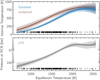 |
Fig. 8 Tint–Teq and PRCB –Teq diagrams in the upper and lower panels, respectively. The dark and light shaded regions present the 68 and 95% credible intervals. Although the analytical approach overestimates the internal temperature at Teq between 1000 and 1800 K, there is a good agreement at Teq < 1000 K and Teq > 1800 K. Due to the increase in the internal temperature with equilibrium temperature, the PRCB moves to lower pressures with increasing Teq, reaching up to ~3 bar for the most irradiated planets. |
7 Discussion
Building on the assumption that hot Jupiters are inflated because of a process leading to high internal luminosity, we infer for each planet the internal luminosity distribution that reproduces the radius given the planet mass and equilibrium temperature from observations and using the mass–heavy-element relation (Thorngren et al. 2016) as a prior for the fraction of heavy elements. We then combine the individual distributions to constrain the population mass–luminosity–radius (MLR) distribution. Assuming that the source of extra heat in the interior is the irradiation by the host star (e.g., tides or magnetic fields), we then compute the fraction of the incident flux ϵ deposited in the interior and study the heating-efficiency–equilibrium-temperature (HEET) distribution for the full population. Finally, as a by-product of our structure model, we can also gain insights into the interior structure of the planets by inferring the distributions of the internal temperature and the pressure at the RCB.
In what follows, in Sect. 7.1 we discuss the consequences of the hot interior hot Jupiters possess on the internal structure. Then we discuss our results within the context of the competing heating mechanisms, mainly ohmic dissipation in Sect. 7.2 and advection of potential temperature in Sect. 7.3. In Sect. 7.4, we give a general comparison with analytical relations and discuss the limitations and caveats of our results in Sect. 7.5.
7.1 Insights into the interior structure of hot Jupiters
We have shown that hot Jupiters have hot interiors, with an internal temperature as high as 800 K. This has important consequences on the location of the RCB, which in turn is important for the heating mechanism. Komacek & Youdin (2017) showed that heat dissipated in the convective layers suppresses cooling and thus enables the planet to maintain a large radius. Heat deposited in the radiative layer, however, does not significantly inhibit cooling. Most it is reradiated away leading therefore to small radii. The location of the RCB is hence important to constrain the minimum depth at which the heat should be deposited and thus the efficiency of the heating mechanism. We find that the RCB is around 100 bar for planets with equilibrium temperatures of about 1000 K, and can reach 3 bar for the highly irradiated planets, which is significantly lower than previous estimates of 1000 bar without accounting for a bloating mechanism (Fortney et al. 2007). Our results are in agreement with T19 based on coupling the heating efficiency relation (TF18) to a planetary interior structure model.
Mechanisms based on transporting heat into the deep interior, such as atmospheric circulation (Showman & Guillot 2002), ohmic dissipation (Batygin & Stevenson 2010), or advection of potential temperature (Tremblin et al. 2017) rely on the existence of winds in the interior. While the extra heat must be deposited in the convective layer in order to inflate the planet (Komacek & Youdin 2017), the actual wind speeds are not constrained from Global Circulation Models (GCMs) due to inaccurate coupling between the atmosphere and deep interior. Recently, Carone et al. (2020) showed that through a better treatment of the lower boundary condition, that is, by accounting for a hot interior, shallow zonal winds are present at 100 bar. With new estimates and better understanding of the internal temperature and pressure at the RCB, the depth of the wind zone and wind speeds can be constrained from GCM models, which in turn will be key inputs to further study the efficiency of the proposed mechanisms.
7.2 Comparison to ohmic dissipation
The general idea of ohmic dissipation is that equilibrium temperatures larger than 1000 K lead to thermally ionized atmospheres that couplesto the magnetic field and in the presence of strong winds produces currents, which then dissipate thermally in the deep interior (Batygin & Stevenson 2010; Batygin et al. 2011). However, in the high equilibrium temperature regime and therefore high atmospheric ionization fraction, ions slow down the winds due to Lorentz force, which in turn decrease the efficiency of ohmic dissipation (Perna et al. 2010a,b). Scaling law relations based on ohmic dissipation showed that indeed the heating efficiency increases with equilibrium temperature until a maximum is reached beyond which the efficiency decreases (Menou 2012), which was also confirmed by TF18 and now in our study. The scaling laws also suggest that the location of the peak depends on the strength of the magnetic field. Therefore, studying the functional form of the HEET distribution provides insights within the context of ohmic dissipation.
Based on our analysis, we find that the HEET distribution can be modeled by a Gaussian function, in agreement with TF18 and with the theoretical predictions. We find however that the location of the peak is at 1860 K, which is higher compared to the work of TF18 that reported the peak around 1566 K (see Table 1). Menou (2012) showed that the transition is a function of the strength of the magnetic field (see his Fig. 4) where stronger magnetic fields push the peak to higher equilibrium temperatures (the peak is at ~ 1800 K for a 30 G field). Ginzburg & Sari (2016) estimate the transition around ~ 1500 K based on analytical models and Rogers & Komacek (2014) at ~1500−1600 K based on magnetohydrodynamic simulations. Yadav & Thorngren (2017) estimate the surface magnetic field strength of hot Jupiters using the energy flux scaling law from Christensen et al. (2009) and account for the extra heat injected using the heating efficiency relation presented by TF18. They found magnetic field strengths around 50− 100 G for the most inflated hot Jupiters. There are no theoretical atmospheric circulation models with such strong magnetic fields, which might hence change the location of the peak. The transition is still not well constrained and might depend on the field strength but the Gaussian distribution is robust and most importantly is prior independent. Future observations of magnetic field strengths could potentially provide a better overview but for now they remain unconstrained from an observational point of view (for a current review see Griessmeier 2017; Lazio 2018).
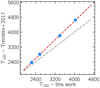 |
Fig. 9 Temperature at 100 bar derived from our PT structures compared to the values from the average PT profiles using 2D circulation models presented by Tremblin et al. (2017) resulting from the advection of potential temperature. All the models correspond to a planet with log g = 2.97 ± 0.15 and increasing stellar incident flux. The gray dashed line shows the 1:1 relation while the red dashed line shows the fit to the data. |
7.3 Comparison to advection of potential temperature
Another source of heat could be the movement of high-entropy fluid parcels deeper into the atmosphere, a process known as advection ofpotential temperature. Within this context, Tremblin et al. (2017) suggested, using two-dimensional (2D) circulation model, that this process leads to a hot interior that can naturally explain the radius anomaly of hot Jupiters. This was further supported recently by 3D GCM simulations (Sainsbury-Martinez et al. 2019). The 2D models show that a stronger stellar incident fluxleads to hotter interior adiabat (see their Fig. 5). We compare our results based on the 1D model to the 2D models by selecting four planets from our sample that matches their simulation parameters, that is, log g = 2.97 ± 0.15 with the corresponding equilibrium temperatures. We do not include the model with the lowest equilibrium temperature (~ 500 K) as it does not match any of the selected systems in our sample. The planets we selected as a function of increasing stellar incident flux are HAT-P-17 b, Corot-4 b, HD209458 b, and HATS-35 b. We then compare the temperatures at 100 bar (T100) using the PT profiles based on the 2D models to the ones based on our 1D model presented in Sect. 3. The results are illustrated in Fig. 9, where the derived temperatures at 100 bar are shown in blue circles and the red dashed line shows the fit to the data. The gray dashed line shows the 1:1 relation on which the points would lie if their model and our data derivedfrom observations would predict identical temperatures. We find that roughly the results agree well with a slope of 1.25, deviating from the 1:1 relation. We note however that these values are model dependent and any change in the treatment of the atmospheric model, for example, including clouds and new opacity sources, will change these values. The temperatures estimated from the average PT profiles using the 2D circulation models are larger than the values predicted by our model, varying from 6 up to 15% for the most irradiated planets. This is expected since the 2D models tend to overestimate the radii compared to the observed ones (Tremblin et al. 2017). Our results concerning the adiabatic profile are also in agreement, where the 2D and 3D atmospheric circulation models suggest a hot adiabat starting at ~10 bar, significantly at lower pressures compared to standard irradiated models (e.g., Fortney et al. 2007). This is in agreement with our findings andconclusions that future GCM models should account for the extra heat in the interior of inflated hot Jupiters and in-line with the work of Carone et al. (2020). We note however that convection is not included in the models of Tremblin et al. (2017). In this context, the RCB should not be interpreted as a Radiative-Convective-Boundary but rather as a proxy for the Radiative-Circulation-Boundary. As such, the energy flux is downward and not upward, which in turn leads to a hotter adiabat.
7.4 General comparison to previous studies
It is useful and informative to compare the results of our model with analytical relations. We consider the analytical approximations of the internal luminosity based on ohmic dissipation (LHuang; Eq. (14) of Huang & Cumming 2012) and thermal tides (LSocrates; Eq. (8) of Socrates 2013):
![Mathematical equation: \begin{align} &L_{\textrm{Huang}}\,{=}\,3 \,{\times}\, 10^{22} \, \textrm{erg \, s^{-1} } \left(\frac{B_{\phi 0}}{10 \, \textrm{G}} \right)^2 \left(\frac{\sigma_t}{10^6 \, \textrm{s^{-1}}} \right)^{-1} \nonumber \\ &\qquad\quad\ \ \ {\times}\, \left(\frac{{T_{\textrm{eq}}}}{1500 \, \textrm{K}} \right) \left(\frac{{R_{\mathrm{p}}}}{{R_{\textrm{J}}}} \right)^4 \left(\frac{{M_{\textrm{p}}}}{{M_{\textrm{J}}}} \right)^{-1}\\ & L_{\textrm{Socrates}}\,{=}\,1.5\,{\times}\, 10^{28} \, \textrm{erg \, s^{-1} } \left(\frac{P}{4 \, \textrm{days}} \right)^{-2} \nonumber \\[2ex] &\qquad\quad\ \ \ \ {\times}\, \left(\frac{{T_{\textrm{eq}}}}{2000 \, \textrm{K}} \right) ^3 \left(\frac{{R_{\mathrm{p}}}}{10^{10} \, \textrm{cm}} \right)^4.\end{align}](/articles/aa/full_html/2021/01/aa38361-20/aa38361-20-eq53.png)
In the aboveequations, Bϕ0 is the toroidal component of the magnetic field at a reference pressure of 10 bar, σt is the electrical conductivity in the dissipation region, and P is the orbital period. To compute LHuang, we fix σt to the nominal value 106 s^-1 and consider two different cases for Bϕ0. In the first case, we fix Bϕ0 to 10 G and in the second case, we compute the mean magnetic field strength at the surface of the dynamo based on the scaling law of Christensen et al. (2009) in the form given by Reiners & Christensen (2010):
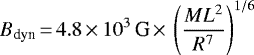 (43)
(43)
where M, L, and R are the mass, luminosity, and radius of the planet normalized to solar units. We assume Bϕ0 = Bdyn. We note that using this relation, Bdyn ranges roughly between 30 and 480 G for our sample, in agreement with the previous estimates of Yadav & Thorngren (2017). We refer to these cases as LHuang, Bfixed and LHuang, Bvar, respectively. It is straightforward then to calculate LSocrates, LHuang, Bfixed and LHuang, Bvar for each hot Jupiter in our sample using the relevant physical properties.
We also examine our results within the context of advection of high-entropy material based on models of Tremblin et al. (2017). Our aim is to compare the internal luminosity of the planets that this mechanism predicts to the internal luminosities derived in Sect. 4.1. Tremblin et al. (2017) computed 2D PT profiles only for four planets with different Teq values. We thus need to estimate the internal luminosity of all the planets based on the model of advection of potential temperature, for which we follow the procedure described next. We first compute the entropy using the SCvH EOS (Saumon et al. 1995) and T100, which was derived from the 2D PT profiles based on four fiducial planets with different Teq (see Sect. 7.3 for more details). Second, we fit a relation between the equilibrium temperatures of the four planets and their estimated entropy. Finally, to convert the entropy into an internal luminosity, we use the entropy–mass–luminosity relation from an updated version of the population synthesis of Mordasini (2018). The second step allows us to compute the entropy for all the selected hot Jupiters in our sample using the observed Teq. Having calculated the entropy and knowing Mp from observations, the last step allows us to compute the internal luminosity of the planets. With this procedure, we therefore calculate the internal luminosity of the planets predicted by this mechanism based on these fits and based on Teq and Mp from observations. We consider three cases for comparison by assuming the planets are composed of H/He and setting the fraction of heavy elements to 0, 10, and 20%. We refer to these models as LTremblin_0, LTremblin_10, and LTremblin_20, respectively. We point out that the values should be taken with caution as there are strong approximations involved in this approach.
Finally, to compare our results to TF18, we use the analytical ϵ(Teq) (Eq. (34) in their paper) to compute ϵ and then estimate LTF18 using Eq. (6).
Figure 10 compares our results to the various studies where the dashed lines are the 1:10, 1:1, and 1:0.1 relations. The predicted luminosities based on the analytical solution of thermal tides as suggested by Socrates (2013) and the advection ofpotential temperature (Tremblin et al. 2017) are on the same order of magnitude as the ones we derive in this work based on observations. The advection of potential temperature (Tremblin et al. 2017) predicts high luminosity values for the leastluminous planets in our sample. This is expected since their model tend to overestimate the radii compared to observations, even for planets with incident flux below the threshold of inflation (stellar incident flux of ~ 2 × 10⁸ erg s−1 cm−2 or Teq ≈ 1000 K).
The relation of Huang & Cumming (2012) based on ohmic dissipation leads to small internal luminosity values. We note that this relation is an order-of-magnitude estimation of the total ohmic power. We therefore caution that these results do not provide evidence against ohmic dissipation, but rather that this relation underestimates the ohmic power. Based on our results and the work of TF18, there is compelling evidence from the HEET relation that ohmic dissipation can explain the radii of hot Jupiters. The ohmic power values estimated by Batygin & Stevenson (2010) and Menou (2012) are up to three orders of magnitude higher than the values predicted by Huang & Cumming (2012) and thus on the same order of magnitude estimated in this work. Moreover, the small internal luminosity values using the relation of Huang & Cumming (2012) could also explain the findings of Lopez & Fortney (2016), where it was shown that the relation did not lead to reinflation of hot Jupiters.
For our models with Lint < 102 LJ, the model of TF18 predicts smaller values of Lint. This difference is a direct consequence of the discrepancy in ϵ as shown in the right panel of Fig. 6, where as discussed in Sect. 6.3 we predict higher heating efficiencies for the least and the most irradiated planets.
Converting the luminosity values to a heating efficiency using Eq. (6), the models of Socrates (2013) and Tremblin et al. (2017) do not lead to a decrease in the heating efficiency at the highest equilibrium temperatures. The former predicts a continuous increase as was shown by TF18 with values as high as 20–25% and the latter seems to increase moderately up to 30, 10, and 2% for Zp = 0, 0.1, and 0.2, respectively. This is expected given the steeper increase in the luminosity values above 104 LJ for both models. These are the highly inflated and highly irradiated hot Jupiters (Rp > 1.4 RJ and Teq > 1900 K). We note that the peak in the HEET distribution in our model occurs close to 1900 K (see Sect. 6.3 and Table 1), beyond which ϵ decreases for higher Teq. This explains why the models of Socrates (2013) and Tremblin et al. (2017) do not predict a Gaussian function, that is, why ϵ does not decrease at high Teq. We stress that these models can nevertheless explain the observed radii of most of the hot Jupiters and can be the dominant mechanisms responsible for inflation even in the absence of the Gaussian function. It could be thus that these mechanisms are too efficient in inflating hot Jupiters at temperatures above than 1900 K. Thermal tides have received less attention within the context of the radius anomaly problem and thus more work is needed to understand the physical regime where this mechanism is efficient.
In summary, we provide evidence that thermal tides and advection of potential temperature can reproduce the large observed radii of most of the hot Jupiters based on the internal luminosity predicted using these models. Moreover, the HEET distribution suggests that ohmic dissipation can also explain the radii of the close-in giant planets (see Sect. 7.2). We therefore conclude that all of these three mechanisms can explain the inflation of hot Jupiters. This is in line with our main goals where we stress that these mechanisms were tested on only a handful of exoplanets and a statistical approach is necessary to confirm or refute these mechanisms for the entire population.
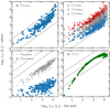 |
Fig. 10 Comparison of the internal luminosity derived in this work from observations and other (theoretical) studies. The solid dashed lines are from top to bottom the 1:10, 1:1, and 1:0.1 relations. The different panels show the results in comparison with analytical relations (Huang & Cumming 2012; Socrates 2013), numerical modeling (Tremblin et al. 2017), and based on a statistical approach similar to ours (TF18). See text for explanations on the different versions of LHuang and LTremblin. Notice the different scales in each panel. The results based on the analytical approximations of Huang & Cumming (2012) underestimate Lint. There is an agreement with TF18, Tremblin et al. (2017), and Socrates (2013) giving thus evidence for advection of potential temperature and thermal tides as possible mechanisms to explain the radius inflation conundrum. |
7.5 Limitations and caveats
There are important caveats and limitations related to this work that should be explicitly mentioned.
Our results and conclusions are based on a simple 1D interior structure model. Hot Jupiters however are tidally locked, which gives rise to a temperature gradient between the day-side and the night-side. The RCB at the night-side might thus be at lower pressures compared to the day-side leading to uneven cooling. As a consequence of that, Spiegel & Burrows (2013) showed using a 1+1D model that the net effect of incorporating night-side cooling leads to higher cooling rates compared to the default 1D models. 2D circulation models also showed that the location of the RCB differs from the day-side to the night-side, which furtherenhances the cooling rate (Rauscher & Showman 2014) and thus requires even higher efficiency to explain the radii of hot Jupiters. This is especially important for the highly irradiated planets as it was shown that the day-side–night-side temperature differences increases with stellar irradiation (Komacek & Showman 2016; Komacek et al. 2017).
In addition, we assume that the heat is deposited in the interior of the planet and we do not account for dissipation in the intermediate layers. A better treatment would be to deposit the heat over a range of depths similar to Ginzburg & Sari (2016) or Komacek & Youdin (2017). Moreover, even though we showed that the Gaussian profile of the HEET distribution is in agreement with ohmic dissipation there are few shortcomings to this. A key component for ohmic dissipation is the electrical conductivity σ, where the ohmic power is proportional to 1∕σ (Batygin & Stevenson 2010). The electrical conductivity increases dramatically in the interior leading to efficient heating only at lower densities and thus at lower pressures. However, the layers that contribute to the inflation are not at the surface where the conductivity is maximum but rather at deeper layers (between 100 and 1000 bar; Batygin et al. 2011). Wu & Lithwick (2013) confirmed these results by showing that heat deposited at 100 bar requires significantly less heating efficiency in comparison to 10 or 3 bar (0.3% compared to 3% and 200%, respectively, see their Fig. 3). It is therefore unclear whether the Gaussian functional form holds for energy dissipated at lower pressures.
The depth of the heating has also direct consequences on the interior structure. For example, Huang & Cumming (2012) included ohmic heating only in the radiative layers deeper than 10 bar and showed that as a consequence of that the RCB moves to deeper pressures. However, their model cannot reproduce the radii of massive planets. Understanding the location of the RCB is crucial as it regulates the planetary cooling rate and thus the contraction rate (Arras & Bildsten 2006; Marleau & Cumming 2014). Future developments of state-of-the-art GCM models that solve the complete equations without approximations and that couple the upper atmosphere with the deep convective layers will provide a complete picture of the underlying physical processes.
Finally, in this work we did not account for observational biases. A large number of the hot Jupiters discovered to date are discovered using ground based telescopes, such as WASP (Pollacco et al. 2006) and the HATNet and HATSouth (Bakos 2018) exoplanet surveys. There is a lack of hot Jupiters with radii smaller than ~ 1.4 RJ around early- and mid-F stars. This is because detecting such planets is still challenging from the ground as the transit depths are shallow and less than 0.5%. Heng (2012) showed that if ohmic dissipation can explain the anomalously large radii of hot Jupiters, then this naturally leads to scatter in the radii at a given stellar incident flux due to variations in the opacity, albedo, cloud/hazes properties, and the magnetic fields strength. It is therefore still not quite clear whether the lack of “medium-inflated” hot Jupiters around F stars is due to observational biases or variations in the efficiency of the heating mechanism. The NASA Transiting Exoplanet Survey Satellite mission (TESS; Ricker et al. 2015) will discover such planets if they exist and will help to better constrain the efficiency of the heating mechanisms either by the lack or existence of such planets. Subsequently high precision follow-up observationswith the CHaracterising ExOPlanet Satellite (CHEOPS; Broeg et al. 2013) will help to get very accurate radii.
8 Conclusion
In this work, we developed a flexible and robust hierarchical Bayesian model to couple the observed physical parameters of hot Jupiters to an interior structure model. The model accounts for observational uncertainties and for the scatter in the relation between planet mass and heavy-element fraction. We validated the statistical method by applying it to synthetic planets based on planet population synthesis and showed that we are able to retrieve the true distribution. We then applied this method to quantify the internal luminosity needed to explain the radii of a sample of 314 hot Jupiters. We tested this model under two different priors (assuming a log-uniform and a linear-uniform distributions for Lint) and showed that the population level distributions are prior independent (Fig. 5). This provides useful and robust constraints on the interior structure of hot Jupiters. We find that such planets tend to have hotter interiors compared to previous assumptions, and as a result, the RCB is located at low pressures, in agreement with recent work by Thorngren et al. (2019) (Fig. 8).
Assuming the planet has reached steady state and assuming that the additional source of heat is the stellar irradiation, we compute the heating efficiency ϵ, defined as the fraction of stellar irradiation deposited into the interior of the planet that is, needed to explain the observed inflated radii. We find that the heating-efficiency–equilibrium-temperature relation is described by a Gaussian function (Fig. 6), in agreement with previous work by TF18, however, the peak is not consistent in both studies. We found that the models of TF18 predict larger radii than our models for Teq > 1500 K, which we attribute due to differences in the atmospheric modeling. The Gaussian-like pattern is more importantly in agreement with theoretical predictions based on the ohmic dissipation model (Menou 2012). We also show that thermal tides (Arras & Socrates 2010; Socrates 2013) and advection of potential temperature (Tremblin et al. 2017) can explain the observations of most of the planets in our sample and thus are possible mechanisms responsible for the anomalously large radii of hot Jupiters (Fig. 10).
To conclude, we provide new insights into the interior of hot Jupiters by coupling observations to theoretical models within a powerful statistical framework. With a better understanding of the interior, we highlight the importance of accounting for the extra heat flux in the interior in 3D GCM models, which will further improve our understanding of wind speeds and hence on the efficiency of the heating mechanisms.
The future of hot Jupiters is exciting and bright. Simulations of the exptected TESS yield (Barclay et al. 2018)predict that TESS will discover more than 250 hot Jupiters suitable for RV follow-up (Rp > 1 RJ) with orbital periods < 10 days orbiting bright stars (V < 14 mag), almost doubling the number of hot Jupiters discovered. The mission already detected few hot Jupiters (e.g., Kossakowski et al. 2019; Wang et al. 2019) with many yet to be discovered. Furthermore, CHEOPS (Broeg et al. 2013) is capable of detecting the phase curves of hot Jupiters, which provide information on the day-night temperature contrast. CHEOPS will therefore play a major role in providing clues into the efficiency of energy transport in hot Jupiter atmospheres (e.g., HD 189733 b; Knutson et al. 2007). With a better understanding of the interior structure of hot Jupiters thanks to the development of flexible and computationally efficient statistical tools, we will be able to provide further constraints on the radius inflation conundrum.
The source code for the hierarchical model is open source11 under the MIT open source software license. Part of the code is still being added and available upon request.
The posterior samples at the population level are also available online12.
Software: corner (Foreman-Mackey 2016), emcee (Foreman-Mackey et al. 2013), Jupyter https://jupyter. org/, matplotlib (Hunter 2007), numpy (van der Walt et al. 2011), petitCODE (Mollière et al. 2015, 2017), pandas (McKinney 2010), scikit-learn (Pedregosa et al. 2011), scipy (Virtanen et al. 2020).
Acknowledgements
P.S., C.M., G.-D.M. acknowledge the support from the Swiss National Science Foundation under grant BSSGI0_155816 “PlanetsInTime”. Parts of this work have been carried out within the framework of the NCCR PlanetS supported by the Swiss National Science Foundation. T.H. and P.M. acknowledge support from the European Research Council under the Horizon 2020 Framework Program via the ERC Advanced Grant Origins 83 24 28. G.-D.M. acknowledges the support of the DFG priority program SPP 1992 “Exploring the Diversity of Extrasolar Planets” (KU 2849/7-1). P.S. would like to thank David Hogg and Morgan Fouesneau for useful discussions related to the importance sampling technique and multilevel modeling and Daniel Thorngren for sharing the posterior distributions of the individual planets and the data used in Fig. 1. P.S. thanks Saavi and Gabriele for exchanging priority time on the aida server.
Appendix A Supplemental information
In Sect. 6.2, we showed that the mass–luminosity–radius (MLR) posterior distribution is similar when assuming Lint follows either a linear-uniform or a log-uniform prior distribution. In this appendix we show that the heating-efficiency–equilibrium temperature (HEET), Tint–Teq, and PRCB–Teq distributions are also similar using both priors. Figures A.1 and A.2 show the HEET and both the Tint–Teq and PRCB–Teq distributions, respectively. Tables A.1 and A.2 present the 68% credible interval values for the model parameters for the MLR distribution assuming linear-uniform and log-uniform priors. Similarly, Table A.3 for the HEET distribution using a 4th degree polynomial, Table A.4 for the Tint–Teq distribution using a Gaussian function, and finally Table A.5 for the PRCB–Teq distribution using a polynomial function.
 |
Fig. A.1 HEET posterior distribution under the linear–uniform (left) and the log–uniform (middle) priors using a Gaussian and 4th degree polynomial. The shaded region shows the 68% credible interval. There is a good agreement between both models using the same prior. To better compare the same model using different priors, the right panel shows the Gaussian models using log (red) and linear (blue) uniform priors. |
68% credible interval values of the parameters for the mass–luminosity–radius (MLR) distribution for the linear– case modeled as a 4th degree polynomial
  where x = Rp.
68% credible interval values of the parameters for the mass–luminosity–radius (MLR) distribution for the log– case modeled as a 4th degree polynomial
  where x = Rp.
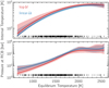 |
Fig. A.2 Tint–Teq and PRCB –Teq diagrams in the upper and lower panels, respectively. The shaded regions show the 95% credible interval. Both distributions are similar at the 95% level using the linear–uniform (red) and the log-uniform (blue) priors. |
68% credible interval values of the parameters for the heating-efficiency–equilibrium temperature (HEET) distribution for the linear– and log–
 cases using the 4th degree polynomial model
  , where x = Teq∕1000.


References
- Arras, P., & Bildsten, L. 2006, ApJ, 650, 394 [NASA ADS] [CrossRef] [Google Scholar]
- Arras, P., & Socrates, A. 2010, ApJ, 714, 1 [Google Scholar]
- Bakos, G. Á. 2018, Handbook of Exoplanets (Cham: Springer), 111 [Google Scholar]
- Baraffe, I., Selsis, F., Chabrier, G., et al. 2004, A&A, 419, L13 [NASA ADS] [CrossRef] [EDP Sciences] [Google Scholar]
- Baraffe, I., Chabrier, G., & Barman, T. 2008, A&A, 482, 315 [NASA ADS] [CrossRef] [EDP Sciences] [Google Scholar]
- Barclay, T., Pepper, J., & Quintana, E. V. 2018, ApJS, 239, 2 [NASA ADS] [CrossRef] [Google Scholar]
- Batygin, K., & Stevenson, D. J. 2010, ApJ, 714, L238 [NASA ADS] [CrossRef] [Google Scholar]
- Batygin, K., Stevenson, D. J., & Bodenheimer, P. H. 2011, ApJ, 738, 1 [NASA ADS] [CrossRef] [Google Scholar]
- Bodenheimer, P., Lin, D. N. C., & Mardling, R. A. 2001, ApJ, 548, 466 [NASA ADS] [CrossRef] [Google Scholar]
- Broeg, C., Fortier, A., Ehrenreich, D., et al. 2013, Eur. Phys. J. Web Conf., 47, 03005 [CrossRef] [EDP Sciences] [Google Scholar]
- Burrows, A., Guillot, T., Hubbard, W. B., et al. 2000, ApJ, 534, L97 [NASA ADS] [CrossRef] [PubMed] [Google Scholar]
- Burrows, A., Hubeny, I., Budaj, J., & Hubbard, W. B. 2007, ApJ, 661, 502 [NASA ADS] [CrossRef] [Google Scholar]
- Carone, L., Baeyens, R., Mollière, P., et al. 2020, MNRAS, 496, 3582 [CrossRef] [Google Scholar]
- Chabrier, G., & Baraffe, I. 2007, ApJ, 661, L81 [Google Scholar]
- Christensen, U. R., Holzwarth, V., & Reiners, A. 2009, Nature, 457, 167 [NASA ADS] [CrossRef] [PubMed] [Google Scholar]
- Collins, K. A., Kielkopf, J. F., & Stassun, K. G. 2017, AJ, 153, 78 [NASA ADS] [CrossRef] [Google Scholar]
- Delrez, L., Santerne, A., Almenara, J. M., et al. 2016, MNRAS, 458, 4025 [NASA ADS] [CrossRef] [Google Scholar]
- Demory, B.-O., & Seager, S. 2011, ApJS, 197, 12 [NASA ADS] [CrossRef] [Google Scholar]
- Dorn, C., Harrison, J. H. D., Bonsor, A., & Hands, T. O. 2019, MNRAS, 484, 712 [Google Scholar]
- Emsenhuber, A., Mordasini, C., Burn, R., et al. 2020, A&A, submitted, [arXiv:2007.05561] [Google Scholar]
- Enoch, B., Collier Cameron, A., & Horne, K. 2012, A&A, 540, A99 [NASA ADS] [CrossRef] [EDP Sciences] [Google Scholar]
- Folkner, W. M., Iess, L., Anderson, J. D., et al. 2017, Geophys. Res. Lett., 44, 4694 [NASA ADS] [CrossRef] [Google Scholar]
- Foreman-Mackey, D. 2016, J. Open Source Softw., 1, 24 [Google Scholar]
- Foreman-Mackey, D., Hogg, D. W., Lang, D., & Goodman, J. 2013, PASP, 125, 306 [Google Scholar]
- Foreman-Mackey, D., Hogg, D. W., & Morton, T. D. 2014, ApJ, 795, 64 [NASA ADS] [CrossRef] [Google Scholar]
- Fortney, J. J., Marley, M. S., & Barnes, J. W. 2007, ApJ, 659, 1661 [NASA ADS] [CrossRef] [Google Scholar]
- Fortney, J. J., Lodders, K., Marley, M. S., & Freedman, R. S. 2008, ApJ, 678, 1419 [NASA ADS] [CrossRef] [Google Scholar]
- Freedman, R. S., Lustig-Yaeger, J., Fortney, J. J., et al. 2014, ApJS, 214, 25 [NASA ADS] [CrossRef] [Google Scholar]
- Ginzburg, S., & Sari, R. 2016, ApJ, 819, 116 [NASA ADS] [CrossRef] [Google Scholar]
- Griessmeier, J. M. 2017, Planetary Radio Emissions VIII, eds. G. Fischer, G. Mann, M. Panchenko, & P. Zarka (Vienna: Austrian Academy of Sciences Press), 285 [Google Scholar]
- Grunblatt, S. K., Huber, D., Gaidos, E. J., et al. 2016, AJ, 152, 185 [NASA ADS] [CrossRef] [Google Scholar]
- Grunblatt, S. K., Huber, D., Gaidos, E., et al. 2017, AJ, 154, 254 [NASA ADS] [CrossRef] [Google Scholar]
- Guillot, T. 2010, A&A, 520, A27 [NASA ADS] [CrossRef] [EDP Sciences] [Google Scholar]
- Guillot, T., & Gautier, D. 2014, ArXiv e-prints, [arXiv:1405.3752] [Google Scholar]
- Guillot, T., & Showman, A. P. 2002, A&A, 385, 156 [NASA ADS] [CrossRef] [EDP Sciences] [Google Scholar]
- Hartman, J. D., Bakos, G. Á., Bhatti, W., et al. 2016, AJ, 152, 182 [NASA ADS] [CrossRef] [Google Scholar]
- Heng, K. 2012, ApJ, 748, L17 [NASA ADS] [CrossRef] [Google Scholar]
- Hogg, D. W., & Foreman-Mackey, D. 2018, ApJS, 236, 11 [NASA ADS] [CrossRef] [Google Scholar]
- Hogg, D. W., Myers, A. D., & Bovy, J. 2010, ApJ, 725, 2166 [NASA ADS] [CrossRef] [Google Scholar]
- Huang, X., & Cumming, A. 2012, ApJ, 757, 47 [NASA ADS] [CrossRef] [Google Scholar]
- Hunter, J. D. 2007, Comput. Sci. Eng., 9, 90 [NASA ADS] [CrossRef] [Google Scholar]
- Jin, S., & Mordasini, C. 2018, ApJ, 853, 163 [NASA ADS] [CrossRef] [Google Scholar]
- Jin, S., Mordasini, C., Parmentier, V., et al. 2014, ApJ, 795, 65 [Google Scholar]
- Knutson, H. A., Charbonneau, D., Allen, L. E., et al. 2007, Nature, 447, 183 [NASA ADS] [CrossRef] [PubMed] [Google Scholar]
- Komacek, T. D., & Showman, A. P. 2016, ApJ, 821, 16 [NASA ADS] [CrossRef] [Google Scholar]
- Komacek, T. D., & Youdin, A. N. 2017, ApJ, 844, 94 [CrossRef] [Google Scholar]
- Komacek, T. D., Showman, A. P., & Tan, X. 2017, ApJ, 835, 198 [NASA ADS] [CrossRef] [Google Scholar]
- Kossakowski, D., Espinoza, N., Brahm, R., et al. 2019, MNRAS, 490, 1094 [CrossRef] [Google Scholar]
- Laughlin, G., Crismani, M., & Adams, F. C. 2011, ApJ, 729, L7 [NASA ADS] [CrossRef] [Google Scholar]
- Lazio, T. J. W. 2018, Handbook of Exoplanets (Cham: Springer), 9 [Google Scholar]
- Li, L., Baines, K. H., Smith, M. A., et al. 2012, J. Geophys. Res. Planets, 117, E11002 [Google Scholar]
- Linder, E. F., Mordasini, C., Mollière, P., et al. 2019, A&A, 623, A85 [NASA ADS] [CrossRef] [EDP Sciences] [Google Scholar]
- Lopez, E. D., & Fortney, J. J. 2016, ApJ, 818, 4 [NASA ADS] [CrossRef] [Google Scholar]
- Loredo, T. J., & Hendry, M. A. 2019, ArXiv e-prints, [arXiv:1911.12337] [Google Scholar]
- Marleau, G. D., & Cumming, A. 2014, MNRAS, 437, 1378 [Google Scholar]
- Marleau, G.-D., Coleman, G. A. L., Leleu, A., & Mordasini, C. 2019, A&A, 624, A20 [NASA ADS] [CrossRef] [EDP Sciences] [Google Scholar]
- Maxted, P. F. L., Anderson, D. R., Doyle, A. P., et al. 2013, MNRAS, 428, 2645 [NASA ADS] [CrossRef] [Google Scholar]
- McKinney, W. 2010, in Proceedings of the 9th Python in Science Conference, eds. Stéfan van der Walt & Jarrod Millman, 56 [Google Scholar]
- Menou, K. 2012, ApJ, 745, 138 [NASA ADS] [CrossRef] [Google Scholar]
- Miller, N., & Fortney, J. J. 2011, ApJ, 736, L29 [NASA ADS] [CrossRef] [Google Scholar]
- Mol Lous, M., & Miguel, Y. 2020, MNRAS, 495, 2994 [CrossRef] [Google Scholar]
- Mollière, P., van Boekel, R., Dullemond, C., Henning, T., & Mordasini, C. 2015, ApJ, 813, 47 [NASA ADS] [CrossRef] [Google Scholar]
- Mollière, P., van Boekel, R., Bouwman, J., et al. 2017, A&A, 600, A10 [NASA ADS] [CrossRef] [EDP Sciences] [Google Scholar]
- Mollière, P., Wardenier, J. P., van Boekel, R., et al. 2019, A&A, 627, A67 [NASA ADS] [CrossRef] [EDP Sciences] [Google Scholar]
- Mordasini, C. 2018, Handbook of Exoplanets (Cham: Springer), 143 [Google Scholar]
- Mordasini, C. 2020, A&A, 638, A52 [CrossRef] [EDP Sciences] [Google Scholar]
- Mordasini, C., Alibert, Y., Klahr, H., & Henning, T. 2012, A&A, 547, A111 [NASA ADS] [CrossRef] [EDP Sciences] [Google Scholar]
- Mordasini, C., Marleau, G. D., & Mollière, P. 2017, A&A, 608, A72 [NASA ADS] [CrossRef] [EDP Sciences] [Google Scholar]
- Muller, S., Helled, R., & Cumming, A. 2020, A&A 638, A121 [CrossRef] [EDP Sciences] [Google Scholar]
- Owen, J. E., & Jackson, A. P. 2012, MNRAS, 425, 2931 [Google Scholar]
- Pedregosa, F., Varoquaux, G., Gramfort, A., et al. 2011, J. Mach. Learn. Res., 12, 2825 [Google Scholar]
- Perna, R., Menou, K., & Rauscher, E. 2010a, ApJ, 719, 1421 [NASA ADS] [CrossRef] [Google Scholar]
- Perna, R., Menou, K., & Rauscher, E. 2010b, ApJ, 724, 313 [NASA ADS] [CrossRef] [Google Scholar]
- Pollacco, D. L., Skillen, I., Collier Cameron, A., et al. 2006, PASP, 118, 1407 [NASA ADS] [CrossRef] [Google Scholar]
- Price-Whelan, A. M., Hogg, D. W., Rix, H.-W., et al. 2018, AJ, 156, 18 [NASA ADS] [CrossRef] [Google Scholar]
- Rauscher, E., & Showman, A. P. 2014, ApJ, 784, 160 [CrossRef] [Google Scholar]
- Reiners, A., & Christensen, U. R. 2010, A&A, 522, A13 [NASA ADS] [CrossRef] [EDP Sciences] [Google Scholar]
- Ricker, G. R., Winn, J. N., Vanderspek, R., et al. 2015, J. Astron. Telesc., Instrum., Syst., 1, 014003 [Google Scholar]
- Rogers, L. A. 2015, ApJ, 801, 41 [NASA ADS] [CrossRef] [Google Scholar]
- Rogers, T. M., & Komacek, T. D. 2014, ApJ, 794, 132 [NASA ADS] [CrossRef] [Google Scholar]
- Sainsbury-Martinez, F., Wang, P., Fromang, S., et al. 2019, A&A, 632, A114 [NASA ADS] [CrossRef] [EDP Sciences] [Google Scholar]
- Saumon, D., Chabrier, G., & van Horn, H. M. 1995, ApJS, 99, 713 [NASA ADS] [CrossRef] [Google Scholar]
- Sestovic, M., Demory, B.-O., & Queloz, D. 2018, A&A, 616, A76 [NASA ADS] [CrossRef] [EDP Sciences] [Google Scholar]
- Showman, A. P., & Guillot, T. 2002, A&A, 385, 166 [NASA ADS] [CrossRef] [EDP Sciences] [Google Scholar]
- Sing, D. K., Lavvas, P., Ballester, G. E., et al. 2019, AJ, 158, 91 [Google Scholar]
- Socrates, A. 2013, ArXiv e-prints, [arXiv:1304.4121] [Google Scholar]
- Southworth, J. 2011, MNRAS, 417, 2166 [NASA ADS] [CrossRef] [Google Scholar]
- Spiegel, D. S.,& Burrows, A. 2013, ApJ, 772, 76 [NASA ADS] [CrossRef] [Google Scholar]
- Thompson, S. L. 1990, Sandia Natl. Lab. Doc. [Google Scholar]
- Thorngren, D. P., & Fortney, J. J. 2018, AJ, 155, 214 [NASA ADS] [CrossRef] [Google Scholar]
- Thorngren, D. P., Fortney, J. J., Murray-Clay, R. A., & Lopez, E. D. 2016, ApJ, 831, 64 [NASA ADS] [CrossRef] [Google Scholar]
- Thorngren, D., Gao, P., & Fortney, J. J. 2019, ApJ, 884, L6 [CrossRef] [Google Scholar]
- Tremblin, P., Chabrier, G., Mayne, N. J., et al. 2017, ApJ, 841, 30 [NASA ADS] [CrossRef] [Google Scholar]
- Valencia, D., Guillot, T., Parmentier, V., & Freedman, R. S. 2013, ApJ, 775, 10 [NASA ADS] [CrossRef] [Google Scholar]
- van der Walt, S., Colbert, S. C., & Varoquaux, G. 2011, Comput. Sci. Eng., 13, 22 [Google Scholar]
- Venturini, J., Alibert, Y., & Benz, W. 2016, A&A, 596, A90 [NASA ADS] [CrossRef] [EDP Sciences] [Google Scholar]
- Virtanen, P., Gommers, R., Oliphant, T. E., et al. 2020, Nat. Methods, 17, 261 [Google Scholar]
- Wahl, S. M., Hubbard, W. B., Militzer, B., et al. 2017, Geophys. Res. Lett., 44, 4649 [NASA ADS] [CrossRef] [Google Scholar]
- Wang, S., Jones, M., Shporer, A., et al. 2019, AJ, 157, 51 [NASA ADS] [CrossRef] [Google Scholar]
- Weiss, L. M., Marcy, G. W., Rowe, J. F., et al. 2013, ApJ, 768, 14 [NASA ADS] [CrossRef] [Google Scholar]
- Wolfgang, A., & Lopez, E. 2015, ApJ, 806, 183 [NASA ADS] [CrossRef] [Google Scholar]
- Wolfgang, A., Rogers, L. A., & Ford, E. B. 2016, ApJ, 825, 19 [NASA ADS] [CrossRef] [Google Scholar]
- Wu, Y., & Lithwick, Y. 2013, ApJ, 763, 13 [NASA ADS] [CrossRef] [Google Scholar]
- Yadav, R. K., & Thorngren, D. P. 2017, ApJ, 849, L12 [NASA ADS] [CrossRef] [Google Scholar]
- Youdin, A. N., & Mitchell, J. L. 2010, ApJ, 721, 1113 [NASA ADS] [CrossRef] [Google Scholar]
When comparing to other work, it is crucial to use the same entropy zero-point or to correct for this. See footnote 2 of Mordasini et al. (2017).
The top line in Eq. (12) is the likelihood probability density function (PDF) and the bottom line is the prior PDF.
It takes around 5 min on a modern laptop to evaluate the upper model for K = 1, that is, without accounting for uncertainties on the x-axis. For K = 2000, it takes around 2 CPU hours on a server using 20 cores.
This is the same red dashed model shown in Fig. 1 in the TF18 paper.
Available at https://github.com/psarkis/bloatedHJs
All Tables
Comparison of the Gaussian function using the log and linear uniform prior along with comparison to TF18 results.
68% credible interval values of the parameters for the mass–luminosity–radius (MLR) distribution for the linear– case modeled as a 4th degree polynomial where x = Rp.
68% credible interval values of the parameters for the mass–luminosity–radius (MLR) distribution for the log– case modeled as a 4th degree polynomial where x = Rp.
68% credible interval values of the parameters for the heating-efficiency–equilibrium temperature (HEET) distribution for the linear– and log– cases using the 4th degree polynomial model , where x = Teq∕1000.
All Figures
|
Fig. 1 Equilibrium temperature–radius diagram (left panel) and mass–radius diagram (right panel) color-coded by entropy for the 314 hot Jupiters selected for our analysis. The solid black and the red dashed lines compare the radii computed using our model completo21 and TF18, respectively. Both models are for a 1 MJ planet with a pure H/He composition with Y = 0.27 at 5 Gyr and without accounting for inflation. The entropy was computed using the observed physical properties and an assumedheavy-element fraction of 0.2. Planets with large radii tend to have high internal entropy, with a weak dependence on planetary mass. |
| In the text | |
|
Fig. 2 Posterior distributions inferred for HD 209458 b using our model (Eq. (12)). The gray dashed lines show the observed value for the relevant parameters. The effect of using different prior distribution leads to different posterior distributions for Lint, ϵ, and Zp. The inferred posterior distributions for the other parameters (L*, Mp, and Rp) are almost identical for both priors since they are constrained well from observations. |
| In the text | |
|
Fig. 3 Left: PDF of the prior on the internal luminosity distributions for WASP-48 b and EPIC-211418728 b under the linear- |
| In the text | |
|
Fig. 4 Model validation on planet population synthesis data. Heating efficiency – equilibrium temperature (HEET) posterior distribution using the linear-uniform (left) and the log-uniform (middle) priors for a Gaussian and 4th degree polynomial. The thick lines denotes the posterior median for the relevant functions and the dashed black line denotesthe true distribution implemented in the Bern population synthesis model, which was used to generate the synthetic data. The dark and light shaded region contains the 68 and 90% credible interval. To better compare the same model using different priors, the right panel shows the Gaussian models using log (red) and linear (blue) uniform priors. The light gray model in the right panel is the inferred posterior distribution in case we do not correct for the choice of prior. Our model is able to retrieve the Gaussian-like function when modeled using a 4th degree polynomial. The posterior median provides a good fit to the true distribution although the linear model predicts a lower heating efficiency. The credible intervals derived are able to accurately constrain the true values of the model parameters. |
| In the text | |
|
Fig. 5 Mass–luminosity–radius (MLR) posterior distribution for four different mass bins showing the median (thick line) and 68% credible interval (shaded area) assuming a uniform prior in log (blue) and linear (red) space. Using either prior leads to almost identical results. The internal luminosity is high with the largest planets having a luminosity approximately four orders of magnitude larger than Jupiter. |
| In the text | |
|
Fig. 6 Left: heating efficiency–equilibrium temperature (HEET) posterior distribution under the linear-uniform prior using a Gaussian function and a 4th degree polynomial. Right: the Gaussian function shown on the left side in comparison to the HEET posterior distribution inferred by TF18. The shaded region show the 68% credible interval. There is a good agreement between the Gaussian and poly models, which shows that indeed the HEET distribution follows a Gaussian function. Our results are in agreement with the findings of TF18 although the peak in our models is shifted to higher equilibrium temperatures. |
| In the text | |
|
Fig. 7 Posterior distributions of the heating efficiency ϵ for all the planets with Teq > 2000 K. The colors indicate planets with Teq < 2250 K and Teq > 2250 K in blue and red, respectively. Six out of the seven planets shown in red favor small heating efficiency values with the most probable value close to ϵ ~ 1%. This provides evidence that the interior structure model disfavor high ϵ values and thus the decrease seen in the HEET distribution is real given our structure model. |
| In the text | |
|
Fig. 8 Tint–Teq and PRCB –Teq diagrams in the upper and lower panels, respectively. The dark and light shaded regions present the 68 and 95% credible intervals. Although the analytical approach overestimates the internal temperature at Teq between 1000 and 1800 K, there is a good agreement at Teq < 1000 K and Teq > 1800 K. Due to the increase in the internal temperature with equilibrium temperature, the PRCB moves to lower pressures with increasing Teq, reaching up to ~3 bar for the most irradiated planets. |
| In the text | |
|
Fig. 9 Temperature at 100 bar derived from our PT structures compared to the values from the average PT profiles using 2D circulation models presented by Tremblin et al. (2017) resulting from the advection of potential temperature. All the models correspond to a planet with log g = 2.97 ± 0.15 and increasing stellar incident flux. The gray dashed line shows the 1:1 relation while the red dashed line shows the fit to the data. |
| In the text | |
|
Fig. 10 Comparison of the internal luminosity derived in this work from observations and other (theoretical) studies. The solid dashed lines are from top to bottom the 1:10, 1:1, and 1:0.1 relations. The different panels show the results in comparison with analytical relations (Huang & Cumming 2012; Socrates 2013), numerical modeling (Tremblin et al. 2017), and based on a statistical approach similar to ours (TF18). See text for explanations on the different versions of LHuang and LTremblin. Notice the different scales in each panel. The results based on the analytical approximations of Huang & Cumming (2012) underestimate Lint. There is an agreement with TF18, Tremblin et al. (2017), and Socrates (2013) giving thus evidence for advection of potential temperature and thermal tides as possible mechanisms to explain the radius inflation conundrum. |
| In the text | |
|
Fig. A.1 HEET posterior distribution under the linear–uniform (left) and the log–uniform (middle) priors using a Gaussian and 4th degree polynomial. The shaded region shows the 68% credible interval. There is a good agreement between both models using the same prior. To better compare the same model using different priors, the right panel shows the Gaussian models using log (red) and linear (blue) uniform priors. |
| In the text | |
|
Fig. A.2 Tint–Teq and PRCB –Teq diagrams in the upper and lower panels, respectively. The shaded regions show the 95% credible interval. Both distributions are similar at the 95% level using the linear–uniform (red) and the log-uniform (blue) priors. |
| In the text | |
Current usage metrics show cumulative count of Article Views (full-text article views including HTML views, PDF and ePub downloads, according to the available data) and Abstracts Views on Vision4Press platform.
Data correspond to usage on the plateform after 2015. The current usage metrics is available 48-96 hours after online publication and is updated daily on week days.
Initial download of the metrics may take a while.