| Issue |
A&A
Volume 644, December 2020
|
|
|---|---|---|
| Article Number | A120 | |
| Number of page(s) | 9 | |
| Section | Interstellar and circumstellar matter | |
| DOI | https://doi.org/10.1051/0004-6361/202039309 | |
| Published online | 10 December 2020 | |
ALMA chemical survey of disk-outflow sources in Taurus (ALMA-DOT)
IV. Thioformaldehyde (H2CS) in protoplanetary discs: spatial distributions and binding energies★
1
INAF, Osservatorio Astrofisico di Arcetri,
Largo E. Fermi 5,
50125
Firenze, Italy
e-mail: This email address is being protected from spambots. You need JavaScript enabled to view it.
2
Univ. Grenoble Alpes, CNRS, Institut de Planétologie et d’Astrophysique de Grenoble (IPAG),
38000
Grenoble, France
3
Dipartimento di Chimica and Nanostructured Interfaces and Surfaces (NIS) Centre, Università degli Studi di Torino,
Via P. Giuria 7,
10125
Torino, Italy
4
INAF, Osservatorio Astrofisico di Torino,
Via Osservatorio 20,
10025
Pino Torinese, Italy
5
Università degli Studi di Firenze, Dipartimento di Fisica e Astronomia,
Via G. Sansone 1,
50019
Sesto Fiorentino, Italy
6
INAF, Istituto di Radioastronomia & Italian ALMA Regional Centre,
Via P. Gobetti 101,
40129
Bologna, Italy
7
European Southern Observatory,
Karl-Schwarzschild-Strasse 2,
85748
Garching bei München, Germany
8
Excellence Cluster Origins,
Boltzmannstrasse 2,
85748
Garching bei München, Germany
Received:
1
September
2020
Accepted:
2
November
2020
Abstract
Context. Planet formation starts around Sun-like protostars with ages ≤1 Myr, but the chemical compositions of the surrounding discs remains unknown.
Aims. We aim to trace the radial and vertical spatial distribution of a key species of S-bearing chemistry, namely H2CS, in protoplanetary discs. We also aim to analyse the observed distributions in light of the H2CS binding energy in order to discuss the role of thermal desorption in enriching the gas disc component.
Methods. In the context of the ALMA chemical survey of disk-outflow sources in the Taurus star forming region (ALMA-DOT), we observed five Class I or early Class II sources with the o-H2CS(71,6−61,5) line. ALMA-Band 6 was used, reaching spatial resolutions ≃40 au, that is, Solar System spatial scales. We also estimated the binding energy of H2CS using quantum mechanical calculations, for the first time, for an extended, periodic, crystalline ice.
Results. We imaged H2CS emission in two rotating molecular rings in the HL Tau and IRAS 04302+2247 discs, the outer radii of which are ~140 au (HL Tau) and 115 au (IRAS 04302+2247). The edge-on geometry of IRAS 04302+2247 allows us to reveal that H2CS emission peaks at radii of 60–115 au, at z = ±50 au from the equatorial plane. Assuming LTE conditions, the column densities are ~1014 cm−2. We estimate upper limits of a few 1013 cm−2 for the H2CS column densities in DG Tau, DG Tau B, and Haro 6–13 discs. For HL Tau, we derive, for the first time, the [H2CS]/[H] abundance in a protoplanetary disc (≃10−14). The binding energy of H2CS computed for extended crystalline ice and amorphous ices is 4258 and 3000–4600 K, respectively, implying thermal evaporation where dust temperatures are ≥50–80 K.
Conclusions. H2CS traces the so-called warm molecular layer, a region previously sampled using CS and H2CO. Thioformaldehyde peaks closer to the protostar than H2CO and CS, plausibly because of the relatively high excitation level of the observed 71,6−61,5 line (60 K). The H2CS binding energy implies that thermal desorption dominates in thin, au-sized, inner and/or upper disc layers, indicating that the observed H2CS emitting up to radii larger than 100 au is likely injected in the gas phase due to non-thermal processes.
Key words: astrochemistry / protoplanetary disks / methods: numerical / ISM: individual objects: HL Tau / ISM: individual objects: IRAS 04302+2247
Reduced datacubes are only available at the CDS via anonymous ftp to cdsarc.u-strasbg.fr (130.79.128.5) or via http://cdsarc.u-strasbg.fr/viz-bin/cat/J/A+A/644/A120
© ESO 2020
1 Introduction
Low-mass star formation is the process starting from a molecular cloud and ending with a Sun-like star with its own planetary system. According to the classical scenario (e.g. Andre et al. 2000; Caselli & Ceccarelli 2012, and references therein), the central object increases its mass through an accretion disc, while a fast jet contributes in removing the angular momentum excess. While the star accretes its mass, part of the material in the disc is incorporated to form planets. As the physical process proceeds, the chemistry evolves towards a complex gas composition (see Ceccarelli et al. 2007; Herbst & van Dishoeck 2009). Several observational programs have been dedicated to the chemical content of protostellar envelopes/discs using both single-dish radiotelescopes and interferometers at millimetre(mm) wavelenghts (IRAM 30-m ASAI, Lefloch et al. 2018; ALMA PILS, Jørgensen et al. 2016; IRAM PdBI CALYPSO, Belloche et al. 2020; IRAM NOEMA SOLIS, Ceccarelli et al. 2017; ALMA FAUST1, Bianchi et al. 2020); the recent IRAM 30-m survey by Le Gal et al. (2020). Nevertheless, relatively little is known about the chemical content of the protoplanetary discs. Tiny outer molecular layers (and therefore small column densities) are formed due to thermal or UV-photodesorption and/or CR-induced desorption (e.g., Semenov & Wiebe 2011; Walsh et al. 2014, 2016; Loomis et al. 2015; Le Gal et al. 2019). More precisely, the disc portions where thermal desorption is expected to rule are in turn determined by the binding energies (BEs) of the species to grains. Different BEs imply different temperatures of the dust which can inject frozen molecules into the gas phase (e.g. Penteado et al. 2017).
Several projects focusing on protoplanetary discs, mainly with ALMA2, have recently come to fruition, leading to the detection of several molecules from CO isotopologues to complex species such as t-HCOOH, CH3 OH, and CH3CN (see Öberg et al. 2013, 2015a,b; Öberg & Bergin 2016; Guilloteau et al. 2016; Favre et al. 2015, 2018, 2019; Fedele et al. 2017; Semenov et al. 2018; Podio et al. 2019, 2020a,b; Garufi et al. 2020). The ALMA images allowed these latter authors to compare the gas and dust distribution, making the first steps in physical–chemical modelling. A breakthrough result provided by ALMA, through (sub)mm array observations of young stellar objects, suggests that planets already start to form during the protostellar phases, that is, before the classical protoplanetary stage at an age of at least 1 Myr. This is indirectely indicated by the presence of rings, gaps, and spirals in discs with ages of less than 1 Myr (see e.g., Sheehan & Eisner 2017; Fedele et al. 2018; Andrews et al. 2018). These substructures have also been observed using molecules, driving studies to sample the molecular components of discs. This is the goal of the ALMA-DOT project (ALMA chemical survey of Disk-Outflow sources in Taurus), which targets Class I or early Class II discs to obtain their chemical characterisation.
The chemistry of S-bearing species is not well understood. In dense gas, which is involved in the star forming process, sulphur is severely depleted (e.g. Wakelam et al. 2004; Phuong et al. 2018; Tieftrunk et al. 1994; Laas & Caselli 2019; van ’t Hoff et al. 2020), that is, by at least two orders of magnitude with respect to the Solar System value [S]/[H] = 1.8 × 10⁻⁵ (Anders & Grevesse 1989). However, the main S-carrier species on dust grains are still unknown. For years, H2 S has been postulated to be the solution, but so far it has not been directly detected on interstellar ices (Boogert et al. 2015). Alternative solutions have been proposed in light of studies focused on protostellar shocks, where dust is sputtered: S, OCS, and H2 CS (e.g. Wakelam et al. 2004; Codella et al. 2005; Podio et al. 2014; Holdship et al. 2016) have been investigated, but again no detection on ices has been reported (Boogert et al. 2015). Regarding the inventory of S-molecules in protoplanetary discs, only four species have been detected, often using single-dish radiotelescopes: CS, SO, H2 S, and H2 CS. More specifically, multiline CS emission has been observed towards approximately ten discs (e.g. Dutrey et al. 1997, 2017; Fuente et al. 2010; Guilloteau et al. 2013, 2016; Teague et al. 2018; Phuong et al. 2018; Semenov et al. 2018; Le Gal et al. 2019; Garufi et al. 2020; Podio et al. 2020a). SO emission has been detected in fewer discs, some of them still associated with accretion, such as for example TMC-1A (e.g. Fuente et al. 2010; Guilloteau et al. 2013, 2016; Sakai et al. 2016; Pacheco-Vázquez et al. 2016; Teague et al. 2018; Booth et al. 2018). On the other hand, only very recently, H2 S and H2 CS were detected and imaged towards multiple discs. Namely, H2S was imaged towards GG Tau A (Phuong et al. 2018), while H2CS was observed with ALMA towards MWC480, and, tentatively, LkCa 15 (Le Gal et al. 2019; Loomis et al. 2020). Further observations of the most likely dust-grain S-carriers are required in the interest of a definitive conclusion.
In this context, the goal of the present project is twofold: (1) to map the H2 CS (thioformaldehyde) spatial distribution in protoplanetary discs in an intermediate phase between Class I and Class II, and (2) to derive the binding energies of H2CS using quantum mechanical calculations for an extended crystalline ice. We focus on H2 CS in an effort to identify S-bearing species able to trace protoplanetary discs. The present article is organised as follows. We first present our observationsand data reduction process (Sect. 2), followed by our observational results (Sect. 3) and the methods and assumptions we used to derive BEs (Sect. 4). In Sect. 5, we discuss our results by comparing the H2 CS maps with (i) those of other molecular species and with (ii) the spatial distributions expected when assuming the thermal desorption process (driven by the BE values) to be the main mechanism leading to H2CS in the gas phase. Finally, Sect. 6 summarises our work.
2 Observations: sample and data reduction
The sample consists of four well-known Class I and one early Class II (e.g. Andre et al. 2000) sources (Guilloteau et al. 2013, 2014): DG Tau, DG Tau B, HL Tau, IRAS 04302+2247, and Haro 6–13 (also known as V 806 Tau). The sources are observed in the context of the ALMA-DOT project, which targets sources: (i) still embedded in a dense envelope and (ii) driving an atomic jet and a molecular outflow. The sources are chemically rich as revealed by IRAM-30m observations detecting CO isotopologues, H2 CO, and CN – plus SO for all but Haro 6–13 – (Guilloteau et al. 2013).
This work is based on ALMA Cycle 4 observations of DG Tau and DG Tau B and Cycle 6 observations of HL Tau, IRAS 04302+2247, and Haro 6-13 (projects 2016.1.00846.S and 2018.1.01037.S, PI: L. Podio). The DG Tau and DG Tau B observations were described by Podio et al. (2019), and Garufi et al. (2020), respectively. All Band 6 observations were taken in an extended array configuration with baselines ranging from 15 m to 1.4 km or from 17 m to 3.7 km. The frequency interval covered by the continuum spectral window included the o–H2 CS(71,6−61,5) line emittingat 244 048.5 MHz, characterised3 by Eup = 60 K, and Sμ2 = 56 D2. A standard data reduction was performed with CASA pipeline version 4.7.2. Self-calibration was performed on the continuum emission and then applied to the continuum-subtracted line datacube. The rms for continuum images are about 68 μJy (HL Tau) and 40 μJy (IRAS 04302+2247). The line spectral cube was produced through TCLEAN. We used robust weighting in order to maximise the spatial resolution, and set a channel width of 1.2 km s−1. The r.m.s. per each channel is about 0.8 mJy beam−1. The synthesised beam (HPBW) is ~0′′.3 × 0′′.3.
3 Observational results
3.1 Continuum and H2CS spatial distributions
Out of the five observed targets, we detected o-H2 CS(71,6−61,5) emission towards two discs, namely HL Tau and IRAS 04302+2247 (herafter IRAS 04302). For DG Tau, DG Tau B, and Haro 6–13, upper limits on H2CS emission are reported in the following sections. As a reference to analyse molecular emission, Fig. 1 (upper panels) reports the dust continuum emission. The well-known HL Tau disc (d = 147 pc; Galli et al. 2018), with an inclination angle i of 47° (e.g. ALMA Partnership 2015; Carrasco-González et al. 2019), is well traced, showing a radius of ~150 au. The dust continuum at 227 GHz peaks (118 mJy beam−1) at α(J2000) = 04h31m38.s44, δ(J2000) = +18°13′57′′.65. On the other hand, the IRAS 04302 disc (Guilloteau et al. 2013; Podio et al. 2020a), located at d = 161 pc (Galli et al. 2019), is more extended (~350 au), and is associated with an almost edge-on geometry, i ~ 90° (Wolf et al. 2003). The coordinates of the continuum peak, 133 mJy beam−1, are α(J2000) = 04h33m16.s47, δ(J2000) = +22°53′20′′.36.
Figure 1 (middle) also reports the intensity integrated maps (moment 0) of the o-H2CS(71,6−61,5) emission as observed towards HL Tau and IRAS 04302, thus providing for the first time the thioformaldeyde radial (HL Tau) and vertical (IRAS 04302) distributions. All the channels showing emission of at least 3σ (see Sect. 2) have been used, namely: 3–11 km s−1 (HL Tau) and 2–10 km s−1 (IRAS 04302). The signal-to-noise ratio (S/N) of the velocity integrated emission is greater than 8 in both sources. For HL Tau, the image clearly shows an H2CS ring around a central dip. The outer radius is about 140 pc, while the dip is confined in the inner ~35 au. For IRAS 04302, the picture provided by the moment 0 map is less clear. The H2 CS emission is confined to the inner 0′′.7, ~115 au. In Sect. 3, we show how kinematics lead us to infer the structure of the emitting region.
Finally, the bottom panels of Fig. 1 report the HL Tau and IRAS 04302 H2 CS(71,6−61,5) spatial distributions of the peak intensity in colour scale, as derived using the moment 8 method4 to improve the images. The moment 8 CASA algorithm was used, collapsing the intensity axis of the ALMA datacube to one pixel and setting the value of that pixel (for RA and Dec) to the maximum value of the spectrum. The moment 8 images confirm the finding from the moment 0 maps. In Sect. 5.2, the spatial distribution is compared with those of other molecular species.
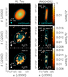 |
Fig. 1 Upper panels: map (cyan contours and colour scale) of the 1.3 mm dust continuum distribution for HL Tau (left) and IRAS 04302+2247 (right) discs. First contours and steps are 3σ (200 μJy beam−1, HL Tau; 115 μJy beam−1, IRAS 04302+2247), and 200σ, respectively. The ellipse in the bottom-left corner shows the ALMA synthesised beam (HPBW): 0′′. 28 × 0′′.25 (PA = –7°), for HL Tau, and 0′′.28 × 0′′.22 (PA = –3°), for IRAS 04302+2247. Middle panels: spatial distribution (moment 0) maps (white contours and colour scale) of the o-H2 CS(71,6–61,5) line based onthe velocity integrated emission (3–11 km s−1, HL Tau, 2–10 km s−1, IRAS 04302+2247) overlaid on the continuum maps (cyan contours). First contours and steps are 5σ (7.5 mJy beam−1 km s−1, HL Tau, and12.5 mJy beam−1 km s−1, IRAS 04302), and 3σ, respectively. The ellipse shows the synthesised beam (HPBW): 0′′.29 × 0′′.27 (PA = 2°) for HL Tau and 0′′.30 × 0′′.26 (PA = 2°) for IRAS 04302+2247. Lower panels: moment 8 maps (white contours and colour scale) of the H2 CS(71,6–61,5) based on the same velocity integrated emission used for the moment 0 maps, overlaid on the continuum maps (cyan contours). First contours and steps are 5σ (3 mJy beam−1 km s−1), and 3σ, respectively. |
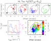 |
Fig. 2 Upper panels: channel maps of the o-H2CS(71, 6–61, 5) blue- and redshifted emission in the HL Tau disc. Each panel shows the emission integrated over a velocity interval of 1.2 km s−1 shifted with respect to the systemic velocity (~+7 km s−1, green) by the value given in the upper-right corner. We report the 3σ contour of the continuum emission in black (Fig. 1). The black triangles indicate where spectra have been extracted. The ellipse shows the synthesised beam (HPBW): 0′′. 29 × 0′′.27 (PA = 2°). First contours and steps correspond to 3σ (2.1 mJy beam−1) and 1σ, respectively. Offsets are derived with respect to the continuum peak. Bottom left panel: o-H2 CS(71, 6–61, 5) spectra in flux and brightness temperature scales (Tb/Fν = 328.593) extracted in the positions marked with a red or blue triangle in the upper panels. Bottom right panel: first-moment map in colour scale. |
3.2 H2CS kinematics
Figures 2 and 3 summarise the kinematics of HL Tau and IRAS 04302 provided by: (i) channel maps, (ii) intensity-weighted mean velocity (moment 1) maps, and (iii) H2 CS spectra as extracted towards the brightest positions. The H2CS in HL Tau is clearly rotating with the blue- and redshifted sides located towards the SE and NW, respectively. The systemic velocity is ~+7.0 km s−1 (in agreement with ALMA Partnership 2015; Wu et al. 2018). The same rotating gradient has been observed using HCO+ (ALMA Partnership 2015; Yen et al. 2019), C18O (Wu et al. 2018), and 13C17O (Booth & Ilee 2020). Also the emission towards the disc of IRAS 04302 shows a rotation pattern. Its almost edge-on orientation allows us to clearly disentangle the red- (southern) and blueshifted (northern) lobes. The systemic velocity estimated from the velocity distribution of the bright H2CO line is + 5.6 km s−1 (Podio et al. 2020a), in good agreement with IRAM 30-m CN, H2CO, CS, and C17O spectra of Guilloteau et al. (2013, 2016). The rotation pattern has been imaged also by Podio et al. (2020a), who found, using CO, H2 CO, and CS emission, a molecular emission which is vertically stratified (see Sect. 4 for the comparison with H2 CS).
The H2CS channel maps show that the emission shifted by less than 2 km s−1 is emitted from the inner 0′′. 5 region, whereas at larger velocities we detect emission up to 1′′.2 from the protostar. This suggests that larger projected velocities (in particular the blueshifted velocity) have a larger projected positional offset from the protostar. In other words, the present dataset suggests that V ∝ R. This is the standard signature of a rotating ring with an inner dip, and not a filled disc for which we would see the opposite trend, with V ∝ R−2. Very recently, Oya & Yamamoto (2020) reported the detection of H2CS in the IRAS16293 A protostellar disc (see also van ’t Hoff et al. 2020). In addition, the present findings closely resemble what was found for the archetypical protostellar disc HH212, which is also close to being edge-on as in IRAS 04302 (e.g. Lee et al. 2019, and references therein). Also in this case, a chemical enrichment in the gas phase associated with rotating rings is revealed by the V ∝ R kinematical feature (see e.g. the recent review by Codella et al. 2019).
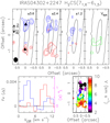 |
Fig. 3 Upper panel: channel maps of the o-H2CS(71,6–61,5) blue- and redshifted emission in the IRAS 04302+2247 disc. Each panel shows the emission integrated over a velocity interval of 1.2 km s−1 shifted with respect to the systemic velocity (~+5.6 km s−1 Podio et al. 2020a, green) by the value given in the upper-right corner. We report the 3σ contour of the continuum emission in black (Fig. 1). The black triangles indicate where spectra have been extracted. The ellipse shows the synthesised beam (HPBW): 0′′. 30 × 0′′.26 (PA = 2°). First contours and steps correspond to 3σ (2.1 mJy beam−1) and 1σ, respectively. Offsets are derived with respect to the continuum peak. Bottom left panel: o-H2 CS(71,6–61,5) spectra in flux and brightness temperature scales (Tb/Fν = 328.593) extracted in the positions marked with a red or blue triangle in the upper panels. Bottom right panel: first-moment map in colour scale. |
3.3 H2CS column densities and abundances
Assuming (i) local thermodynamic equilibrium (LTE) and (ii) optically thin emission, the column densities of the H2 CS are derived. The first assumption is well justified as the H2 gas density in the molecular layers is larger than 107 cm−3 (see e.g. Walsh et al. 2014; Le Gal et al. 2019), i.e. well above the critical density of the considered o-H2CS(71,6–61,5) line (ncr ~ a few 104 cm−3) in the 20–150 K range5. The second assumption is justified as models indicate an abundance (with respect to H) of H2 CS lower than 10−10 (Le Gal et al. 2019; Loomis et al. 2020).
In HL Tau, the observed emitting area is 1.35 arcsec2 (from the moment 0 map) and the flux is 148 mJy km s−1 (2.6 K km s−1). Le Gal et al. (2019) estimated an H2CS rotational temperature between 20 and 80 K in the MWC 480 disc. We conservatively adopted a temperature between 20 and 150 K. An ortho-to-para ratio of 3, i.e. the statistical value, was assumed (as done by Le Gal et al. 2019). We find a total H2 CS column density  (averaged on the emitting area) of 0.9–1.4 × 1014 cm−2. For IRAS 04302 the emitting area is smaller with respect to HL Tau, namely 0.72 arcsec2, and the flux is ≃78 mJy km s−1 (2.5 K km s−1). The column density
  is, similarly to HL Tau, ≃1014 cm−2. These values can also be considered as an a posteriori check that the observed H2 CS emission is optically thin. Indeed, by assuming kinetic temperatures larger than 20 K and densities larger than 107 cm−3, the large velocity gradient approach confirms that column densities around 1014 cm−2 imply an opacity of ≤ 0.1 for the o-H2CS(71,6–61,5) line. These column density estimates are a factor 30 higher than those measured by Le Gal et al. (2019) and Loomis et al. (2020) towards the massive disc MWC 480 (3 × 1012 cm−2). However, as reported by the authors, their spatial resolution is not high enough to evaluate the presence of a central dip, which could cause an underestimate the H2CS column density.
For HL Tau, a further step can be taken given that Booth & Ilee (2020) published an ALMA map of the 13C17O(3–2) emission at a similar angular scale to that of our H2 CS maps. The 13C17O spatial distribution agrees well with that of H2CS. The emission is considered optically thin, given that its abundance ratio with respect to 12C16O is 8.3 × 10⁻⁶ (Milam et al. 2005). Taking the 13C17O flux density of 10–20 mJy beam−1 km s−1, and an excitation temperature, as for H2 CS, in the 20–150 K range, we derive NCO ≃ 5–10 × 1023 cm−2. Using [CO]/[H] = 5 × 10⁻⁵, we find a H2CS abundance (with respect to H) of X(H2CS) ≃ 10−14. A comparison with the H2CS abundances predicted by disc chemistry is challenging, given that this latter depends significantly on the initial composition of the S-species, which can vary by orders of magnitude (see e.g. Fedele & Favre 2020). Vice versa, the present measured H2 CS abundances will hopefully be used in future chemical models to constrain their initial conditions.
Finally, the upper limits on the H2CS column densities in DG Tau, DG Tau B, and Haro 6-13, derived taking the 5σ level of the moment 0 maps and using all the assumptions described above, are:  ≤ 2 × 1013 cm−2 (DG Tau B) and
  ≤ 4 × 1013 cm−2 (DG Tau and Haro 6-13).
4 Binding energies: ice modelling and computational methods
We computed the H2CS and CS BEs, adopting a proton-ordered (P-ice) crystalline model (Casassa et al. 1997) for the bulk ice. The ice surface where the adsorption takes place was simulated by a finite slab model of the (010) surface cut out from the bulk P-ice crystal, as recently proposed by Ferrero et al. (2020) to predict the BEs of a set of 21 molecules using the periodic ab initio program CRYSTAL17 (Dovesi et al. 2018). CRYSTAL17 adopts localised (Gaussian) basis functions that allow the surfaces to be simulated as true 2D systems, without including fake replicas of the slab separated by artificial voids. The surface slab model is sufficiently thick (number of water layers) to ensure a converged surface energy (energy penalty to cut the surface from the bulk ice). The choice of a crystalline ice model goes against the overwhelming evidence that ice in the interstellar environment is amorphous in nature (AWS). There are two main reasons that hinder the adoption of an AWS phase at the modelling level: (i) the experimental atomistic structure of the AWS is unknown; and (ii) any AWS model should be based on a very large unit cell to mimic the disordered nature of the ice. Point (i) means that the model cannot be derived from experimental evidence and therefore any model is somehow arbitrary. Point (ii) implies that very expensive calculations are needed to cope with the large unit cells. In the following, we propose a simplified strategy to derive the values of the BEs for the H2 CS and CS molecules as adsorbed on AWS, without the need to run expensive calculations, but taking advantage of the results of Ferrero et al. (2020) on the analogous CO and H2CO molecules, in which both crystalline and AWS models were studied.
First, we set up the starting locations of H2CS and CS molecules at the ice surface using the optimised positions of the analogous CO and H2 CO molecules after Ferrero et al. (2020) and then fully optimising the structures. We choose the HF-3c method, which combines the Hartree-Fock Hamiltonian with the minimal basis set MINI-1 (Tatewaki & Huzinaga 1980) supplemented by three a posteriori corrections for: (i) the basis set superposition error (BSSE) arising when localised Gaussian functions are used to expand the basis set (Jansen & Ros 1969; Liu & McLean 1973); (ii) the dispersive interactions; and (iii) short-ranged deficiencies due to the adopted minimal basis set (Sure & Grimme 2013). The resulting optimised unit cell of the ice (010) surface is shown in Fig. 4, together with the mapping of the electrostatic potential (ESP) computed at HF-3c level of theory. The ESP reveals the oxygen-rich (red color, ESP < 0) and proton-rich (blue color, ESP > 0) regions, acting as, respectively, H-bond acceptors and donors with respect to specific adsorbates.
In order to get accurate BEs, the HF-3c structures were used to compute single-point energy evaluations at B3LYP-D3(BJ) level of theory (Becke 1993). A dispersion interaction is included through the D3 correction, with the Becke-Johnson damping scheme (Grimme et al. 2010). The Ahlrichs’ triple-zeta quality VTZ basis set supplemented with a double set of polarization functions (Schäfer et al. 1992) was adopted to define the final B3LYP-D3(BJ)/A-VTZ*//HF-3c model chemistry. BEs were also corrected for BSSE.
For H2CS, the most stable structure shows a symmetric involvement of the CH2S molecule with the ice surface, in which the C-H bonds act as weak H-donors toward the surface oxygen atoms, while the S atom acts as a H-bond acceptor at the dangling surface OH groups. For CS, the adsorption occurs through the C-end with a very long H-bond with the dangling ice OH group. Any attempt to engage the CS molecule through the S-end of the molecule evolved spontaneously to the C-end one. Obviously, the relatively simple structure of the crystalline P-ice does not allow us to explore alternative configurations to those described, at variance with the results for an AWS model which would be expected to provide many times more adsorption sites of different strength. Furthermore, due to the long range order of the water molecules in the crystalline ice, the H-bond interactions will cooperate to enhance the H-bond donor(acceptor) character of the surface water molecules, giving very high(low) values of the ESP (see Fig. 4). This means that the BEs resulting from the crystalline model should be taken as an upper limit, as shown by Ferrero et al. (2020). As anticipated, to mitigate the deficiencies of the crystalline ice model we resort to data from the work by Ferrero et al. (2020) for the analogous CO and H2 CO molecules (with respect to CS and H2CS treated here) adsorbed on the AWS model. As expected, these latter authors found a relatively complex adsorption scenario at AWS in comparison to that occurring at the P-ice surface. For CO, five different adsorption sites have been characterised; for H2 CO, up to eight different adsorption sites were predicted. Obviously, each of these adsorption sites provides different values of the BE and in the limit of verylarge AWS models, the BE values will obey a certain distribution. It is clear that a similar study should be carried out for CS and H2CS, but instead, as anticipated, we resort to a simplified scheme to estimate the BE values for the AWS, without actually running any calculation.
First, from the data by Ferrero et al. (2020), we worked out two scaling factors (0.859 and 0.775, respectively) connecting the BE of the CO and H2CO analogues computed for the P-ice to their corresponding averaged BE values for the AWS model. Subsequently, by assuming the same scaling factors for the present CS and H2CS cases, we scaled the BEs for the crystalline ice to estimate their averaged values on the AWS model. In agreement with the CO and H2 CO cases, the BE-AWS for CS and H2CS are smaller than those for the crystalline ice. Table 1 reports the derived BEs on crystalline (H2 CS: 4258 K; CS: 3861 K) and AWS (H2CS: 3000-4600 K; CS: 2700–4000 K) ice for both H2CS and CS.
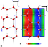 |
Fig. 4 HF-3c optimised P-ice slab model. The adsorption crystallographic plane is the Miller (010) one. Panel A: side view along the b lattice vector. Panel B: top view of the 2 × 1 supercell (|a| = 9.065 Å and |b| = 7.154 Å) along with its ESP map. Colour code: +0.02 atomic unit (blue, positive), 0.00 atomic unit (green, neutral) and –0.02 atomic unit (red, negative). |
H2CS and CS BEs (Kelvin) derived for the crystalline (CRY) and amorphous (AWS) ice models.
5 Discussion
5.1 Comparison with previous BE measurements
Interstellar molecules are formed either through gas-phase reactions or directly on grain surfaces. Regardless of the formation route, gaseous molecules freeze out into the grain mantles on timescales that depend on the density and temperatureof the gas and dust as well as the molecule BE. Thus, in cold and dense regions, as in the outer disc regions and in the layers close to the disc midplane, icy mantles envelope the dust grains. The frozen molecules can then be injected into the gas phase via three processes (see e.g. Walsh et al. 2014): (i) thermal desorption, (ii) UV-photodesorption and/or CR-induced desorption, and (iii) reactive desorption. The first process occurs inside the so-called snow lines, which is the location where the dust temperature is high enough to allow the species to sublimate.
Regarding H2CO, its BE has been experimentally measured on amorphous water surface (AWS) through a thermal desorption process by Noble et al. (2012), for example, to be 3260 ± 60 K, and was also estimated via theoretical computations on AWS and crystalline ice models by Ferrero et al. (2020), who found zero-point-corrected BEs (see Sect. 4) in the 3071–6194 K range for the AWS case, therefore bracketing the experimental value. The BE for the crystalline ice falls at 5187 K, in the higher regime of the AWS range.
Following the described procedure, for H2CS we find BE values of 4258 and 3000–4600 K for the crystalline and AWS ice models, respectively. For CS, we find slightly lower values: 3861 K (crystalline) and 2700–4000 K (AWS). Table 1 compares our results with the available literature data, all coming from computer simulations. The BEs computed by Das et al. (2018), who adopted a tetramer of water molecules to simulate the ice, are at the lower end of our computed BEs range, whereas the BE computed by Wakelam et al. (2017) based on one single water molecule and corrected with an empirical factor, lies at the higher end of our range.
Based on the new computations that we present in Sect. 4 and using a BE ranging from 3000 to 4600 K, H2 CS is expected to thermally sublimate in regions of the disc where the dust temperature exceeds ~50 to ~80 K, respectively. We emphasise that the dispersion in our computed BEs reflects the different possible sites of adsorption of H2 CS, and it is therefore physical and not due to a computational uncertainty (see the discussion in Ferrero et al. 2020). Although we cannot a priori say how many sites are populated with each different BE, we can conservatively assume that H2 CS molecules should remain frozen in regions of the disc with dust temperatures lower than 50–80 K. The fact that H2 CS emission is seen up to outer radii of ~140 au (HL Tau) and ~115 au (IRAS 04302) suggests that non-thermal processes are likely responsible for the presence of H2 CS in the gas in those disc regions.
5.2 Comparison between H2CS, CS, and H2CO
The formation routes of H2CS were recently summarised by Le Gal et al. (2019), who used the gas–grain chemical model Nautilus (Wakelam et al. 2016) supported by the gas chemical dataset KIDA (Wakelam et al. 2015), and by Fedele & Favre (2020), who adopted the thermo-chemical model DALI (Bruderer et al. 2012) coupled with the chemical network UMIST (Woodall et al. 2007). Generally, H2 CS is mainly (99%) formed in the gas phase via neutral-neutral reaction of atomic S with CH3. On the other hand, CS in discs is also thought to be mainly formed in the gas phase, through reactions starting with small hydrocarbons interacting with S+ (in upper disc layers) or S (in inner slabs). Finally, H2CO can be formed on grains due to hydrogenation processes as well and in the gas phase by oxygen reacting with CH3, in an analogous way to S + CH3 → H2 CS (see e.g. Fedele & Favre 2020, and references therein).
For the IRAS 04302 disc, the H2CS vertical intensity profile can be compared with those of CS and formaldehyde (H2 CO); see Podio et al. (2020a). To this end, we averaged the emission radially over 3 pixels (0′′. 18, corresponding to ~29 au) around the selected radius. Figure 5 shows a comparison obtained at 60 and 115 au from the protostar. We note that the H2CS intensity has been multiplied by the factor reported in the labels in order to better compare with those of o-H2CO and CS. The vertical distribution of H2CS (black) shows an asymmetry with respect to the disc midplane (i.e. z = 0), with the emission from the eastern disc side being brighter than in the western side by a factor 1.8 at 60 au radial distance and a factor 1.5 at 115 au. The same asymmetry in the vertical distribution is observed in the H2 CO (blue) and CS (red) emission, and all three species peak at a disc height, z, of about 50 au. This suggests that, at our resolution, the emission from H2 CS, H2 CO, and CS originates from the same disc layer. As discussed by Podio et al. (2020a), the bulk of the H2 CO and CS emission originates from the disc molecular layer where molecules are either released from dust grains orare formed in the gas phase. Given that H2 CS is co-spatial with H2CO and CS and that all three molecules can be efficiently formed in the gas phase using small hydrocarbons (e.g. CH3), we suggest that H2CS may form in similar way.
The comparison between the moment 0 distributions of H2 CS and H2 CO (Podio et al. 2020a) is also instructive (see Fig. 6), revealing slightly different radial distributions of the two molecules. The H2 CO (and CS) emission extends radially out to ~480 au and peaks at ~120 au, while the H2 CS emission is radially confined in the inner 115 au with a peak at ~70 au. The radial distribution of H2CS suggests that the o-H2CS(71,6–61,5) line probes an inner portion of the IRAS 04302 disc, possibly due to a higher Eup (of 60 K) with respect to those of the o-H2CO(31,2–21,1) and CS(5–4) (of 33–35 K). Only further observations of a species using different excitation lines will shed light on this hypothesis.
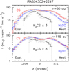 |
Fig. 5 Vertical intensity profile z of H2 CS (black) compared with those of CS(5–4) (red) and o-H2CO(31,2−21,1) (blue), from Podio et al. (2020a). Only fluxes above 3σ confidence are shown. The H2CS intensity has been scaled in order to better compare its profile with those of o-H2 CO and CS. The inner 1′′.8 region is shown, with the positive (negative) values sampling the eastern (western) side. The angular resolution is 0′′. 25 (40 au). The profiles are obtained at ~60 au (upper panel) and 115 au (lower panel) from the protostar. |
6 Conclusions
We present the first images of the radial (HL Tau) and vertical (IRAS 04302) spatial distribution of the o-H2CS emission as observed towards Class I protoplanetary discs using ALMA on a Solar System scale. These observations were performed in the context of the ALMA chemical survey of Disk-Outflow sources in the Taurus star forming region (ALMA-DOT). H2 CS is confined to a rotating ring with an inner dip towards the protostar: the outer radii are 140 au (HL Tau) and 115 au (IRAS 04302). The edge-on geometry of IRAS 04302 allows us to reveal that H2 CS emission peaks at r = 60–115 au, which is at z = ±50 au from the equatorial plane. Assuming LTE conditions, the column densities are ~1014 cm−2. For HL Tau, we derived, for the first time, the [H2 CS]/[H] abundance in a protoplanetary disc (≃10−14). The o-H2CS(71,6−61,5) line emits where the emission of CS(5–4) and o-H2CO(31,2−21,1) is brighter (Podio et al. 2020a), that is, the so-called warm molecular layer. H2 CS emission peaks closer to the protostar with respect to H2CO and CS, possibly because of the higher energy of the upper level (60 K) of the observed transition with respect to those of H2 CO and CS (33–35 K), which requires higher gas temperature, hence favouring the emission from the inner disc regions.
The present work also provides the H2CS and CS BEs as computed for the first time for an extended crystalline ice (4258 K for H2 CS, and 3861 K for CS) and estimated for an AWS model using recipes from previous studies (Ferrero et al. 2020) to be in the 3000–4600 K and 2700–4000 K ranges, respectively. In turn, for ~1 L⊙ protostars, this implies that radially thermal desorption rules in an inner region, while vertically only a thin upper layer is sufficiently hot (see e.g. Walsh et al. 2014; Le Gal et al. 2019). In conclusion, the observed H2 CS, and more precisely that detected at radii up to more than 100 au, is likely released into the gas because of non-thermal processes (photodesorption, CR-induced desorption, and/or reactive-desorption).
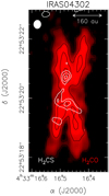 |
Fig. 6 Spatial distribution (moment 0) maps (white contours) of the o-H2CS(71,6–61,5) line (see Fig.1) overlaid on the o-H2CO(31,2−21,1) reported by Podio et al. (2020a), in black contours and red scale. Symbols are as in Fig. 1. |
Acknowledgements
We thank the anonymous referee for instructive discussion and suggestions. This paper uses the ADS/JAO.ALMA 2016.1.00846.S and ADS/JAO.ALMA 2018.1.01037.S (PI: L. Podio) ALMA data. ALMA is a partnership of ESO (representing its member states), NSF (USA) and NINS (Japan), together with NRC (Canada), MOST and ASIAA (Taiwan), and KASI (Republic of Korea), in cooperation with the Republic of Chile. This work was supported by the European Research Council (ERC) under the European Union’s Horizon 2020 research and innovation programmes: (i) “The Dawn of Organic Chemistry” (DOC), grant agreement No 741002, and (ii) “Astro-Chemistry Origins” (ACO), Grant No 811312. C.F. acknowledges financial support from the French National Research Agency in the framework of the Investissements d’Avenir program (ANR-15-IDEX-02), through the funding of the “Origin of Life” project of the Univ. Grenoble-Alpes. D.F. acknowledges financial support from the Italian Ministry of Education, Universities and Research, project SIR (RBSI14ZRHR).
References
- ALMA Partnership (Brogan, C. L., et al.) 2015, ApJ, 808, L3 [NASA ADS] [CrossRef] [Google Scholar]
- Anders, E., & Grevesse, N. 1989, Geochim. Cosmochim. Acta, 53, 197 [Google Scholar]
- Andre, P., Ward-Thompson, D., & Barsony, M. 2000, Protostars & Planets IV (Tucson, AZ: University of Arizona Press) [Google Scholar]
- Andrews, S. M., Huang, J., Pérez, L. M., et al. 2018, ApJ, 869, L41 [NASA ADS] [CrossRef] [Google Scholar]
- Becke, A. D. 1993, J. Chem. Phys., 98, 1372 [NASA ADS] [CrossRef] [Google Scholar]
- Belloche, A., Maury, A. J., Maret, S., et al. 2020, A&A, 635, A198 [CrossRef] [EDP Sciences] [Google Scholar]
- Bianchi, E., Chandler, C. J.. Ceccarelli, C., et al. 2020, MNRAS, 498, L87 [CrossRef] [Google Scholar]
- Boogert, A. C. A., Gerakines, P. A., & Whittet, D. C. B. 2015, Ann. Rev., 53, 541 [Google Scholar]
- Booth, A. S., & Ilee, J. D. 2020, MNRAS, 493, L108 [CrossRef] [Google Scholar]
- Booth, A. S., Walsh, C., Kama, M., et al. 2018, A&A, 611, A16 [NASA ADS] [CrossRef] [EDP Sciences] [Google Scholar]
- Bruderer, S., van Dishoeck, E. F., Doty, S. D., & Herczeg, G. J. 2012, A&A, 541, A91 [NASA ADS] [CrossRef] [EDP Sciences] [Google Scholar]
- Carrasco-González, C., Sierra, A., Flock, M., et al. 2019, ApJ, 883, 71 [NASA ADS] [CrossRef] [Google Scholar]
- Casassa, S., Ugliengo, P., & Pisani, C. 1997, J. Chem. Phys., 106, 8030 [CrossRef] [Google Scholar]
- Caselli, P., & Ceccarelli, C. 2012, A&ARv, 20, 56 [Google Scholar]
- Ceccarelli, C., Caselli, P., Herbst, E., Tielens, A. G. G. M., & Caux, E. 2007, Protostars and Planets V, eds. B. Reipurth, D. Jewitt, & K. Keil (Tucson, AZ: University of Arizona Press), 47 [Google Scholar]
- Ceccarelli, C., Caselli, P., Fontani, F., et al. 2017, ApJ, 850, 176 [NASA ADS] [CrossRef] [Google Scholar]
- Codella, C., Bachiller, R., Benedettini, M., et al. 2005, MNRAS, 361, 244 [NASA ADS] [CrossRef] [Google Scholar]
- Codella, C., Ceccarelli, C., Lee, C.-F., et al. 2019, ACS Earth Space Chem., 3, 2110 [CrossRef] [Google Scholar]
- Das, A., Sil, M., Gorai, P., Chakrabarti, S. i. K., & Loison, J. C. 2018, ApJS, 237, 9 [NASA ADS] [CrossRef] [Google Scholar]
- Dovesi, R., Orlando, R., Erba, A., et al. 2018, Wiley Interdiscip. Rev. Comput. Mol. Sci., 176 [Google Scholar]
- Dutrey, A., Guilloteau, S., & Guelin, M. 1997, A&A, 317, L55 [NASA ADS] [Google Scholar]
- Dutrey, A., Guilloteau, S., Piétu, V., et al. 2017, A&A, 607, A130 [NASA ADS] [CrossRef] [EDP Sciences] [Google Scholar]
- Favre, C., Bergin, E. A., Cleeves, L. I., et al. 2015, ApJ, 802, L23 [NASA ADS] [CrossRef] [Google Scholar]
- Favre, C., Fedele, D., Semenov, D., et al. 2018, ApJ, 862, L2 [NASA ADS] [CrossRef] [Google Scholar]
- Favre, C., Fedele, D., Maud, L., et al. 2019, ApJ, 871, 107 [NASA ADS] [CrossRef] [Google Scholar]
- Fedele, D., & Favre, C. 2020, A&A, 638, A110 [CrossRef] [EDP Sciences] [Google Scholar]
- Fedele, D., Carney, M., Hogerheijde, M. R., et al. 2017, A&A, 600, A72 [NASA ADS] [CrossRef] [EDP Sciences] [Google Scholar]
- Fedele, D., Tazzari, M., Booth, R., et al. 2018, A&A, 610, A24 [NASA ADS] [CrossRef] [EDP Sciences] [Google Scholar]
- Ferrero, S., Zamirri, R., Ceccarelli, C., et al. 2020, ApJ, 904, 11, [CrossRef] [Google Scholar]
- Fuente, A., Cernicharo, J., Agúndez, M., et al. 2010, A&A, 524, A19 [NASA ADS] [CrossRef] [EDP Sciences] [Google Scholar]
- Galli, P. A. B., Loinard, L., Ortiz-Léon, G. N., et al. 2018, ApJ, 859, 33 [NASA ADS] [CrossRef] [Google Scholar]
- Galli, P. A. B., Loinard, L., Bouy, H., et al. 2019, A&A, 630, A137 [NASA ADS] [CrossRef] [EDP Sciences] [Google Scholar]
- Garufi, A., Podio, L., Codella, C., et al. 2020, A&A 636, A65 [CrossRef] [EDP Sciences] [Google Scholar]
- Grimme, S., Antony, J., Ehrlich, S., & Krieg, H. 2010, J. Chem. Phys., 132, 154104 [NASA ADS] [CrossRef] [PubMed] [Google Scholar]
- Guilloteau, S., Di Folco, E., Dutrey, A., et al. 2013, A&A, 549, A92 [NASA ADS] [CrossRef] [EDP Sciences] [Google Scholar]
- Guilloteau, S., Simon, M., Piétu, V., et al. 2014, A&A, 567, A117 [NASA ADS] [CrossRef] [EDP Sciences] [Google Scholar]
- Guilloteau, S., Reboussin, L., Dutrey, A., et al. 2016, A&A, 592, A124 [NASA ADS] [CrossRef] [EDP Sciences] [Google Scholar]
- Herbst, E., & van Dishoeck, E. F. 2009, ARA&A, 47, 427 [NASA ADS] [CrossRef] [Google Scholar]
- Holdship, J., Viti, S., Jimenez-Serra, I., et al. 2016, MNRAS, 463, 802 [NASA ADS] [CrossRef] [Google Scholar]
- Jansen, H., & Ros, P. 1969, Chem. Phys. Lett., 3, 140 [NASA ADS] [CrossRef] [Google Scholar]
- Jørgensen, J. K., van der Wiel, M. H. D., Coutens, A., et al. 2016, A&A, 595, A117 [NASA ADS] [CrossRef] [EDP Sciences] [Google Scholar]
- Laas, J. C., & Caselli, P. 2019, A&A, 624, A108 [CrossRef] [EDP Sciences] [Google Scholar]
- Lee, C.-F., Li, Z.-Y., & Turner, N. J. 2019, Nat. Astron., 466, 24 [NASA ADS] [CrossRef] [Google Scholar]
- Lefloch, B., Bachiller, R., Ceccarelli, C., et al. 2018, MNRAS, 477, 4792 [NASA ADS] [CrossRef] [Google Scholar]
- Le Gal, R., Öberg, K. I., Loomis, R. A., Pegues, J., & Bergner, J. B. 2019, ApJ, 876, 72 [NASA ADS] [CrossRef] [Google Scholar]
- Le Gal, R., Öberg, K. I., Huang, J., et al. 2020, ApJ, 898, 131 [CrossRef] [Google Scholar]
- Liu, B., & McLean, A. D. 1973, J. Chem. Phys., 59, 4557 [NASA ADS] [CrossRef] [Google Scholar]
- Loomis, R. A., Cleeves, L. I., Öberg, K. I., Guzman, V. V., & Andrews, S. M. 2015, ApJ, 809, L25 [NASA ADS] [CrossRef] [Google Scholar]
- Loomis, R. A., Öberg, K. I., Andrews, S. M., et al. 2020, ApJ, 893, 101 [CrossRef] [Google Scholar]
- Maeda, A., Medvedev, I. R., Winnewisser, M., et al. 2008, ApJS, 176, 543 [NASA ADS] [CrossRef] [Google Scholar]
- Milam, S. N., Savage, C., Brewster, M. A., Ziurys, L. M., & Wyckoff, S. 2005, ApJ, 634, 1126 [NASA ADS] [CrossRef] [Google Scholar]
- Müller, H. S. P., Schlöder, F., Stutzki, J., & Winnewisser, G. 2005, J. Mol. Struct., 742, 215 [NASA ADS] [CrossRef] [Google Scholar]
- Noble, J. A., Theule, P., Mispelaer, F., et al. 2012, A&A, 543, A5 [NASA ADS] [CrossRef] [EDP Sciences] [Google Scholar]
- Öberg, K. I., & Bergin, E. A. 2016, ApJ, 831, L19 [NASA ADS] [CrossRef] [Google Scholar]
- Öberg, K. I., Boamah, M. D., Fayolle, E. C., et al. 2013, ApJ, 771, 95 [NASA ADS] [CrossRef] [Google Scholar]
- Öberg, K. I., Furuya, K., Loomis, R., et al. 2015a, ApJ, 810, 112 [NASA ADS] [CrossRef] [Google Scholar]
- Öberg, K. I., Guzmán, V. V., Furuya, K., et al. 2015b, Nature, 520, 198 [NASA ADS] [CrossRef] [PubMed] [Google Scholar]
- Oya, Y., & Yamamoto, S. 2020, ArXiv e-prints [arXiv:2010.01273] [Google Scholar]
- Pacheco-Vázquez, S., Fuente, A., Baruteau, C., et al. 2016, A&A, 589, A60 [NASA ADS] [CrossRef] [EDP Sciences] [Google Scholar]
- Penteado, E. M., Walsh, C., & Cuppen, H. M. 2017, ApJ, 844, 71 [NASA ADS] [CrossRef] [Google Scholar]
- Phuong, N. T., Chapillon, E., Majumdar, L., et al. 2018, A&A, 616, L5 [NASA ADS] [CrossRef] [EDP Sciences] [Google Scholar]
- Podio, L., Lefloch, B., Ceccarelli, C., Codella, C., & Bachiller, R. 2014, A&A, 565, A64 [NASA ADS] [CrossRef] [EDP Sciences] [Google Scholar]
- Podio, L., Bacciotti, F., Fedele, D., et al. 2019, A&A, 623, L6 [Google Scholar]
- Podio, L., Garufi, A., Codella, C., et al. 2020a, A&A, 642, L7 [CrossRef] [EDP Sciences] [Google Scholar]
- Podio, L., Garufi, A., Codella, C., et al. 2020b, A&A, 644, A119 [CrossRef] [EDP Sciences] [Google Scholar]
- Sakai, N., Oya, Y., López-Sepulcre, A., et al. 2016, ApJ, 820, L34 [NASA ADS] [CrossRef] [Google Scholar]
- Schäfer, A., Horn, H., & Ahlrichs, R. 1992, J. Chem. Phys., 97, 2571 [CrossRef] [Google Scholar]
- Schöier, F. L., van der Tak, F. F. S., van Dishoeck, E. F., & Black, J. H. 2005, A&A, 432, 369 [NASA ADS] [CrossRef] [EDP Sciences] [Google Scholar]
- Semenov, D., & Wiebe, D. 2011, ApJS, 196, 2 [NASA ADS] [CrossRef] [Google Scholar]
- Semenov, D., Favre, C., Fedele, D., et al. 2018, A&A, 617, A28 [NASA ADS] [CrossRef] [EDP Sciences] [Google Scholar]
- Sheehan, P. D., & Eisner, J. A. 2017, ApJ, 840, L12 [NASA ADS] [CrossRef] [Google Scholar]
- Sure, R., & Grimme, S. 2013, J. Comput. Chem., 34, 1672 [CrossRef] [Google Scholar]
- Tatewaki, H., & Huzinaga, S. 1980, J. Comput. Chem., 1, 205 [CrossRef] [Google Scholar]
- Teague, R., Henning, T., Guilloteau, S., et al. 2018, ApJ, 864, 133 [NASA ADS] [CrossRef] [Google Scholar]
- Tieftrunk, A., Pineau des Forets, G., Schilke, P., & Walmsley, C. M. 1994, A&A, 289, 579 [Google Scholar]
- van ’t Hoff, M. L. R., van Dishoeck, E. F., Jørgensen, J. K., & Calcutt, H. 2020, A&A, 633, A7 [CrossRef] [EDP Sciences] [Google Scholar]
- Wakelam, V., Caselli, P., Ceccarelli, C., Herbst, E., & Castets, A. 2004, A&A, 422, 159 [NASA ADS] [CrossRef] [EDP Sciences] [Google Scholar]
- Wakelam, V., Loison, J. C., Herbst, E., et al. 2015, ApJS, 217, 20 [NASA ADS] [CrossRef] [Google Scholar]
- Wakelam, V., Ruaud, M., Hersant, F., et al. 2016, A&A, 594, A35 [NASA ADS] [CrossRef] [EDP Sciences] [Google Scholar]
- Wakelam, V., Bron, E., Cazaux, S., et al. 2017, Mol. Astrophys., 9, 1 [Google Scholar]
- Walsh, C., Millar, T. J., Nomura, H., et al. 2014, A&A, 563, A33 [NASA ADS] [CrossRef] [EDP Sciences] [Google Scholar]
- Walsh, C., Loomis, R. A., Öberg, K. I., et al. 2016, ApJ, 823, L10 [NASA ADS] [CrossRef] [Google Scholar]
- Wiesenfeld, L., & Faure, A. 2013, MNRAS, 432, 2573 [NASA ADS] [CrossRef] [Google Scholar]
- Wolf, S., Padgett, D. L., & Stapelfeldt, K. R. 2003, ApJ, 588, 373 [NASA ADS] [CrossRef] [Google Scholar]
- Woodall, J., Agúndez, M., Markwick-Kemper, A. J., & Millar, T. J. 2007, A&A, 466, 1197 [NASA ADS] [CrossRef] [EDP Sciences] [Google Scholar]
- Wu, C.-J., Hirano, N., Takakuwa, S., Yen, H.-W., & Aso, Y. 2018, ApJ, 869, 59 [NASA ADS] [CrossRef] [Google Scholar]
- Yen, H.-W., Gu, P.-G., Hirano, N., et al. 2019, ApJ, 880, 69 [NASA ADS] [CrossRef] [Google Scholar]
Atacama Large Millimeter Array: https://www. almaobservatory.org
The spectral parameters (Maeda et al. 2008) are taken from the Cologne Database for Molecular Spectroscopy (Müller et al. 2005).
Using scaled H2CO collisional rates from Wiesenfeld & Faure (2013), see Schöier et al. (2005).
All Tables
H2CS and CS BEs (Kelvin) derived for the crystalline (CRY) and amorphous (AWS) ice models.
All Figures
|
Fig. 1 Upper panels: map (cyan contours and colour scale) of the 1.3 mm dust continuum distribution for HL Tau (left) and IRAS 04302+2247 (right) discs. First contours and steps are 3σ (200 μJy beam−1, HL Tau; 115 μJy beam−1, IRAS 04302+2247), and 200σ, respectively. The ellipse in the bottom-left corner shows the ALMA synthesised beam (HPBW): 0′′. 28 × 0′′.25 (PA = –7°), for HL Tau, and 0′′.28 × 0′′.22 (PA = –3°), for IRAS 04302+2247. Middle panels: spatial distribution (moment 0) maps (white contours and colour scale) of the o-H2 CS(71,6–61,5) line based onthe velocity integrated emission (3–11 km s−1, HL Tau, 2–10 km s−1, IRAS 04302+2247) overlaid on the continuum maps (cyan contours). First contours and steps are 5σ (7.5 mJy beam−1 km s−1, HL Tau, and12.5 mJy beam−1 km s−1, IRAS 04302), and 3σ, respectively. The ellipse shows the synthesised beam (HPBW): 0′′.29 × 0′′.27 (PA = 2°) for HL Tau and 0′′.30 × 0′′.26 (PA = 2°) for IRAS 04302+2247. Lower panels: moment 8 maps (white contours and colour scale) of the H2 CS(71,6–61,5) based on the same velocity integrated emission used for the moment 0 maps, overlaid on the continuum maps (cyan contours). First contours and steps are 5σ (3 mJy beam−1 km s−1), and 3σ, respectively. |
| In the text | |
|
Fig. 2 Upper panels: channel maps of the o-H2CS(71, 6–61, 5) blue- and redshifted emission in the HL Tau disc. Each panel shows the emission integrated over a velocity interval of 1.2 km s−1 shifted with respect to the systemic velocity (~+7 km s−1, green) by the value given in the upper-right corner. We report the 3σ contour of the continuum emission in black (Fig. 1). The black triangles indicate where spectra have been extracted. The ellipse shows the synthesised beam (HPBW): 0′′. 29 × 0′′.27 (PA = 2°). First contours and steps correspond to 3σ (2.1 mJy beam−1) and 1σ, respectively. Offsets are derived with respect to the continuum peak. Bottom left panel: o-H2 CS(71, 6–61, 5) spectra in flux and brightness temperature scales (Tb/Fν = 328.593) extracted in the positions marked with a red or blue triangle in the upper panels. Bottom right panel: first-moment map in colour scale. |
| In the text | |
|
Fig. 3 Upper panel: channel maps of the o-H2CS(71,6–61,5) blue- and redshifted emission in the IRAS 04302+2247 disc. Each panel shows the emission integrated over a velocity interval of 1.2 km s−1 shifted with respect to the systemic velocity (~+5.6 km s−1 Podio et al. 2020a, green) by the value given in the upper-right corner. We report the 3σ contour of the continuum emission in black (Fig. 1). The black triangles indicate where spectra have been extracted. The ellipse shows the synthesised beam (HPBW): 0′′. 30 × 0′′.26 (PA = 2°). First contours and steps correspond to 3σ (2.1 mJy beam−1) and 1σ, respectively. Offsets are derived with respect to the continuum peak. Bottom left panel: o-H2 CS(71,6–61,5) spectra in flux and brightness temperature scales (Tb/Fν = 328.593) extracted in the positions marked with a red or blue triangle in the upper panels. Bottom right panel: first-moment map in colour scale. |
| In the text | |
|
Fig. 4 HF-3c optimised P-ice slab model. The adsorption crystallographic plane is the Miller (010) one. Panel A: side view along the b lattice vector. Panel B: top view of the 2 × 1 supercell (|a| = 9.065 Å and |b| = 7.154 Å) along with its ESP map. Colour code: +0.02 atomic unit (blue, positive), 0.00 atomic unit (green, neutral) and –0.02 atomic unit (red, negative). |
| In the text | |
|
Fig. 5 Vertical intensity profile z of H2 CS (black) compared with those of CS(5–4) (red) and o-H2CO(31,2−21,1) (blue), from Podio et al. (2020a). Only fluxes above 3σ confidence are shown. The H2CS intensity has been scaled in order to better compare its profile with those of o-H2 CO and CS. The inner 1′′.8 region is shown, with the positive (negative) values sampling the eastern (western) side. The angular resolution is 0′′. 25 (40 au). The profiles are obtained at ~60 au (upper panel) and 115 au (lower panel) from the protostar. |
| In the text | |
|
Fig. 6 Spatial distribution (moment 0) maps (white contours) of the o-H2CS(71,6–61,5) line (see Fig.1) overlaid on the o-H2CO(31,2−21,1) reported by Podio et al. (2020a), in black contours and red scale. Symbols are as in Fig. 1. |
| In the text | |
Current usage metrics show cumulative count of Article Views (full-text article views including HTML views, PDF and ePub downloads, according to the available data) and Abstracts Views on Vision4Press platform.
Data correspond to usage on the plateform after 2015. The current usage metrics is available 48-96 hours after online publication and is updated daily on week days.
Initial download of the metrics may take a while.