| Issue |
A&A
Volume 644, December 2020
|
|
|---|---|---|
| Article Number | A92 | |
| Number of page(s) | 7 | |
| Section | Astrophysical processes | |
| DOI | https://doi.org/10.1051/0004-6361/202039308 | |
| Published online | 04 December 2020 | |
Ionization potential depression and ionization balance in dense carbon plasma under solar and stellar interior conditions
1
College of Science, Zhejiang University of Technology, Hangzhou Zhejiang, 310023 PR China
e-mail: jlzeng@zjut.edu.cn
2
Graduate school of China Academy of engineering Physics, Beijing 100193, PR China
e-mail: jmyuan@gscaep.ac.cn
3
Department of Physics, College of Liberal Arts and Sciences, National University of Defense Technology, Changsha Hunan 410073, PR China
Received:
1
September
2020
Accepted:
12
October
2020
Recent quantitative experiments on the ionization potential depression (IPD) in dense plasma show that the observational results are difficult to explain with the widely used analytical models for plasma screening. Here, we investigate the effect of plasma screening on the IPD and ionization balance of dense carbon plasma under solar and stellar interior conditions using our developed consistent nonanalytical model. The screening potential can be primarily attributed to the free electrons in the plasma and is determined by the microspace distribution of these free electrons. The ionization balance is determined by solving the Saha equation, including the effect of IPD. The predicted IPD and average ionization degree are larger than those obtained using the Stewart–Pyatt model for mass densities that are greater than 3.0 g cm−3. Under solar interior conditions, our results are in better agreement with the Ecker–Kröll model at electron temperatures and densities lower than 250 eV and 2.1 × 1023 cm−3 and in the best agreement with the ion-sphere model at 303 eV and 4.3 × 1023 cm−3. Finally, our results are compared with those obtained via a recent experiment on a CH-mixture plasma that has been compressed six times. The predicted average ionization degree of C in a CH mixture agrees better with the experiment than the Stewart–Pyatt and Thomas–Fermi models when the screening from free electrons contributed by hydrogen atoms is included. Our results provide useful information concerning the ionization balance and can be applied to investigate the opacity and equations of state for dense plasma under the solar and stellar interior conditions.
Key words: Sun: interior / stars: interiors / atomic data / atomic processes / dense matter
© ESO 2020
1. Introduction
The ionization potential and ionization balance of hot dense plasma play vital roles in understanding the solar and stellar interiors, brown dwarfs, giant planets, inertial confinement fusion (Hurricane 2014), and the interaction of intense X-ray lasers with solid-density matter (Seddon et al. 2017). In dense systems, the effective potential of an electron in an atom or ion is modified by the surrounding charged particles; thus, ionization potential depression (IPD) can be attributed to plasma screening. We note that IPD is a crucial physical quantity to determine the ionization balance in dense systems, which is considerably difficult to describe accurately. The Stewart–Pyatt (SP) model (Stewart & Pyatt 1966) interpolates between the Debye–Hückel model (Debye & Hückel 1923) at a low density and high temperature and the ion-sphere (IS) model (Rozsnyai 1972) at a high density and low temperature; the SP model captures most of the essential physics associated with plasma screening. Therefore, this model has been widely applied in the plasma field. However, recent quantitative experiments on IPD (Ciricosta et al. 2012, 2016; Fletcher et al. 2014; Kraus et al. 2016) indicate that the model underestimates IPD. An experiment using solid-density aluminum at a temperature of ∼100 eV (Ciricosta et al. 2012) shows that the IPDs predicted by the Ecker–Kröll model (Ecker & Kröll 1963) are in much better agreement with the experimental values than those of the SP model (Stewart & Pyatt 1966). However, laser-driven shock experiments on aluminum plasmas in the density range of 1.2–9.0 g cm−3 at a higher temperature of ∼600 eV using the ORION laser system (Hoarty & Allan 2013) suggest that both of these analytical models cannot explain the experimental observations, although the SP model agrees better with the experiment than the Ecker-Kröll model. Later experimental investigations (Ciricosta et al. 2016; Fletcher et al. 2014; Kraus et al. 2016) show that the widely used analytical models (Stewart & Pyatt 1966; Rozsnyai 1972; Ecker & Kröll 1963; Debye & Hückel 1923) fail to explain these experiments. Thus, they are not applicable to the solid-density plasma. Hence, the opacity calculations using the Debye–Hückel model (Debye & Hückel 1923) may be unreliable because of the inaccurate atomic structure and ionization balance (Gao et al. 2011).
This has stimulated renewed theoretical investigations on IPD (Preston et al. 2013; Son et al. 2014; Iglesias 2014; Hansen et al. 2014; Crowley 2014; Calisti et al. 2015; Vinko et al. 2014; Hu 2017; Stransky 2016; Lin et al. 2017; Rosmej 2018; Kasim et al. 2018; Ali et al. 2018; Röpke et al. 2019; Lin 2019). An accurate description of IPD is essential for determining the number of bound states available to an embedded atom and plays a crucial role in determining the charge-state distribution and ionization balance. The information about ionization balance is important for determining the physical properties of the equations of state and opacity. However, little is known about the effect of improved IPD on the ionization balance of dense plasma. Furthermore, the relation between the improved IPD and ionization balance must be established.
Carbon is the second most abundant metal element in the Sun. Accurate information concerning the IPD and ionization balance of C plasma is vital for providing accurate inputs to the standard solar model (Bahcall & Ulrich 1988; Guenther et al. 1992). Thus, the discrepancies between the observed and predicted solar structures can be resolved using more accurate opacity (Basu & Antia 2008; Serenelli et al. 2009). The internal structure predicted by the updated standard solar model disagrees with the helioseismic observations (Bahcall et al. 2004). It is difficult to accurately predict the ionization balance under solar and stellar interior conditions (Kraus et al. 2016). The dense carbon and oxygen cores of the white-dwarf stars of the hot-DQ class are surrounded by an envelope, which is mostly comprised of carbon (Dufour et al. 2007; Fontaine & Van Horn 1976). The ionization balance of dense C plasma affects the equations of state (Andrea et al. 2020) and opacity, influencing the properties of the convection zones of the pulsating white-dwarf stars. To benchmark the ionization balance of C plasma, Kraus et al. (2016, 2019) developed an experimental platform to accurately measure the IPD via spectrally resolved X-ray scattering. These results have important implications (e.g., modeling ablators in inertial confinement fusion as well as many astrophysical objects and in studies regarding the physical properties of hot dense plasmas such as the equation of state and opacity) for investigations under extreme solar and stellar interior conditions and research on inertial confinement fusion.
Herein, we investigate the IPD and ionization balance of C plasma under the solar and stellar interior conditions using the plasma screening potential obtained previously (Zeng et al. 2020). This is a nonanalytical model of plasma screening potential on which the energy shifts of the levels and cross sections of microscopic atomic processes, including photoionization and electron-impact excitation and ionization, can be investigated. The plasma screening potential is obtained based on the free-electron microspace distribution, which is determined by the chemical potential of dense plasma in an average-atom model (Yuan 2002). The IPDs predicted by our model (Zeng et al. 2020) and the experimental values of the solid-density Si plasma (Ciricosta et al. 2016) exhibit good agreement. Our theoretical model is validated by comparing the average ionization degree predictions with the experimental results (Kraus et al. 2016).
2. Theoretical method
An atom embedded in a dense-plasma environment experiences an additional screening induced by the plasma particles of free electrons and ions. This screening potential is assumed to be predominantly contributed by free electrons in the plasma; hence, the screening potential is determined by the charge density of free electrons (Zeng et al. 2020; Li et al. 2008) (atomic units are used unless specified otherwise)
![$$ \begin{aligned} V_{\rm scr}(r) = -\frac{Z}{r}\!+\!4\pi \!\left[\frac{1}{{r }}\int _0^{r } {r_1 }\! +\! \int _{r}^{R_0 } r_1 \rho (r_1 )\right]\mathrm{d}r_1\! -\! \frac{3}{2}\left[\frac{3}{\pi }\rho (r)\right]^{{1 \mathord {\left. \right. } 3}}, \end{aligned} $$](/articles/aa/full_html/2020/12/aa39308-20/aa39308-20-eq1.gif)
where Z is the nuclear charge of the considered atom and its radius is determined by the ion number density ni of the plasma as  . The free-electron charge density abides by the Fermi–Dirac distribution:
where c denotes the speed of light in vacuum, k is the free-electron momentum, μ is the chemical potential of plasma,  , and V(r) is the total potential which includes the contribution of Vscr(r). The chemical potential associated with plasma in local thermodynamic equilibrium can be determined via the Saha equation using a detailed level accounting approximation (Gao et al. 2013) or an average atomic model (Yuan 2002). The exchange-correlation functionals of Dharma-Wardana and Taylor (Dharma-Wardana & Taylor 1981) were employed to determine the potential of an average atom. A central potential approximation has been assumed for the screening potential.
For an isolated atom (IA), the atomic structure and properties are determined by the effective single-electron Dirac equation.

where HD and VIA(r) are the single-electron Dirac Hamiltonian and the effective potential of the IA, respectively. Furthermore, ψ(r) is the wave function. The single-electron effective potential VIA(r) is usually obtained through multiple iterations of the Dirac equation.
For a screened atom in a dense-plasma environment, we solved the effective single-electron Dirac equation with the screening potential Vscr(r) being included in the single-electron effective potential. For isolated and screened atoms, the wave function ψ(r) was constructed from the one-electron Dirac spinors.
where n, κ, and m are the principal, relativistic angular, and magnetic quantum numbers of the electron orbital, respectively; Pnκ(r) and Qnκ(r) are the large and small components of the radial wave functions, respectively; and χκm(θ, ψ, σ) is a two-component spherical spinor.
The large and small components of the radial wave functions were determined by the following coupled radial equations:
where α denotes the fine-structure constant and εnκ is the energy eigenvalue of the one-electron orbital. Both the bound and continuum electron orbitals were determined using the same potential of the isolated or screened atoms (Gu 2008). In the above equation, V(r) is considered to be VIA(r) for IA and Vscr(r) for the screened atom.
The IPDs of different ionization stages were obtained by the difference in the ionization potentials of the isolated and screened atoms, which were determined by solving Dirac Eq. (3). These quantities were used to solve the Saha equation.
where Ne is the number density of free electrons, ϕi is the ionization potential of the isolated ionization stage i, and Δϕi is the IPD induced by the plasma environment obtained according to the above procedure. For comparison, the IPDs obtained by the analytical models (Stewart & Pyatt 1966; Rozsnyai 1972; Ecker & Kröll 1963; Debye & Hückel 1923) were used to solve the above Saha equation. Furthermore, Ze and Zi are the partition functions of free electrons and the ionization stage i, respectively:
where gj, i and Ej, i are the statistical weights and energies of level j, respectively, belonging to the ionization stage i. The sum of Zi was calculated over all the available bound states determined by the plasma environment. To determine the available bound states, we performed calculations on the photoionization cross sections with the explicit inclusion of the plasma screening potential in the Dirac equation and we obtained the level structures of the ionization stages i and i + 1. The ionization potential of the ionization stage i was determined by the energy difference of the respective ground levels of i and i + 1. Thus the potential induced by the plasma environment was put directly into the Hamiltonian of the physical system and then the Dirac equation was solved with the plasma screening effect being considered. The ionization potential with the inclusion of plasma screening determines the highest valence electron orbital (with a principal and angular quantum numbers of nmax and lmax) which is still bound in the ion under the given plasma environment. The available bound states of the ionization stage i are made up of levels belonging to the ground configuration and all possible excitations to electron orbitals up to nmaxlmax. The Saha equation was solved under the particle-conservation constraint

and the condition of electric neutrality
Here, N is the total population and qi is the charge of ion stage i. The ionization balance of mixture plasma can be determined by including all pure elements in the Saha equation (Li et al. 2015).
3. Results and discussion
3.1. Dense carbon plasma under solar interior conditions
The Sun, being the best-known star, has always been considered as a reference prototype for other stars. Herein, we investigate the effect of the screening potential on the atomic structure, IPD, and ionization balance for dense C plasma under solar interior conditions. We consider C plasma at electron temperatures and densities of 120 eV and 4.30 × 1022 cm−3, 189.00 eV and 8.70 × 1022 cm−3, 251 eV and 2.06 × 1023 cm−3, 303 eV and 4.32 × 1023 cm−3, 373 eV and 1.06 × 1024 cm−3, and 496 eV and 3.51 × 1024 cm−3. These plasma conditions are deduced from the standard solar model (Bahcall & Ulrich 1988; Guenther et al. 1992) at radius fractions of 0.796 R⊙, 0.7133 R⊙, 0.6195 R⊙, 0.5442 R⊙, 0.4597 R⊙, and 0.3529 R⊙, respectively. The dominant charge states in the plasma under these plasma conditions are the C4+ and C5+ ionization stages.
In Tables 1 and 2, we provide level energies and ionization potentials for the isolated and screened atoms of C4+ and C5+, which are immersed in the aforementioned plasma environment. For an IA, the data are obtained from the NIST database (Kramida et al. 2020). Electron orbitals with a principal quantum number larger than 2 (3s, 3p, 3d, etc.) start to merge into the continuum region below an electron temperature of 373 eV and a density of 1.06 × 1024 cm−3. Above this temperature and density, the 2s and 2p orbitals start to become delocalized due to plasma screening.
Level energies and ionization potential (IP; in eV) for the isolated atom (IA) and screened atom of C4+ embedded in C plasmas at an electron temperature and density of 120 eV and 4.3 × 1022 cm−3 (A), 189 eV and 8.7 × 1022 cm−3 (B), 250 eV and 2.1 × 1023 cm−3 (C), 303 eV and 4.3 × 1023 cm−3 (D), and 373 eV and 1.1 × 1024 cm−3 (E).
Level energies and ionization potential (IP; in eV) for the isolated atom (IA) and screened atom of C5+ embedded in carbon plasmas at an electron temperature and density of 120 eV and 4.3 × 1022 cm−3 (A), 189 eV and 8.7 × 1022 cm−3 (B), 250 eV and 2.1 × 1023 cm−3 (C), 303 eV and 4.3 × 1023 cm−3 (D), and 373 eV and 1.1 × 1024 cm−3 (E).
Significant IPDs can be observed for C4+ and C5+ under solar interior conditions. With the increasing plasma temperature and density toward the inner core of the Sun, the ionization potential (IP) of C4+ decreased from 392.091 eV for the IA to 349.545 eV at 120 eV and 4.3 × 1022 cm−3, 340.157 eV at 189 eV and 8.7 × 1022 cm−3, 325.109 eV at 250 eV and 2.1 × 1023 cm−3, 309.762 eV at 303 eV and 4.3 × 1023 cm−3, and 291.666 eV at 373 eV and 1.1 × 1024 cm−3. Under the condition of 303 eV and 4.3 × 1023 cm−3, the level energies belonging to the configurations of 1s2s and 1s2p (in the energy range of 294.491 eV–303.659 eV) are just below the IP of 309.762 eV. Above the electron temperature and density of 373 eV and 1.1 × 1024 cm−3, the plasma-screening effect is so strong that the energies of the 1s2s and 1s2p levels are greater than the IP. The 2s and 2p electron orbitals become delocalized and merge into the continuum region.
Plasma screening shows larger energy shifts with increasing density and different effects in the case of different electron orbitals for a specific ionization stage. Plasma screening shows a red shift for the level energies of C4+ and C5+, which is predicted to be 0.854, 1.223, 2.273, and 4.345 eV for the inter-combination line of  of C4+ and 0.422, 0.833, 2.343, and 4.240 eV for the dipole-allowed transition line of
  of C4+ at 120 eV and 4.3×1022 cm−3, 189 eV and 8.7 × 1022 cm−3, 250 eV and 2.1 × 1023 cm−3, and 303 eV and 4.3 × 1023 cm−3, respectively. For C5+, the shift is predicted to be 0.663, 1.229, 2.922, and 3.954 eV for the transition line of
  and 0.476, 0.883, 2.102, and 3.398 eV for
  under the aforementioned plasma conditions.
Figure 1 shows our predicted IPDs of C3+–C5+ when immersed in C plasma under the solar interior conditions and the results obtained using the Debye–Hückel (Debye & Hückel 1923), SP (Stewart & Pyatt 1966), IS (Rozsnyai 1972), and Ecker–Kröll (Ecker & Kröll 1963) models. The ionization potentials decrease considerably when the ions are immersed in a dense-plasma environment. A large difference is observed for different plasma screening models. Under all the given plasma conditions, the Debye–Hückel and Ecker–Kröll models predicted the lowest and highest IPDs, respectively. The Debye–Hückel model can be applied to weakly coupled plasma but not to dense plasma. For densities lower than 2.06 × 1023 cm−3, our predicted IPDs are in optimal agreement with the Ecker–Kröll model (Figs. 1a–c). However, with the increasing temperature and density, our predicted IPDs become smaller than those of the Ecker–Kröll model (Figs. 1d–f). At an electron temperature and density of 373 eV and 1.06 × 1024 cm−3, our model and the IS model exhibit good agreement (Rozsnyai 1972). The IPDs predicted by our model are in better agreement with the SP model (Stewart & Pyatt 1966) with the further increase in plasma density at 496 eV and 3.51 × 1024 cm−3.
 |
Fig. 1. Ionization potential depressions of C plasma at electron temperatures and densities of 120 eV and 4.30 × 1022 cm−3 (a), 189.00 eV and 8.70 × 1022 cm−3 (b), 251 eV and 2.06 × 1023 cm−3 (c), 303 eV and 4.32 × 1023 cm−3 (d), 373 eV and 1.06 × 1024 cm−3 (e), and 496 eV and 3.51 × 1024 cm−3 (f). These plasma conditions are deduced from the standard solar model (Bahcall & Ulrich 1988; Guenther et al. 1992) at radius fractions of 0.796 R⊙, 0.7133 R⊙, 0.6195 R⊙, 0.5442 R⊙, 0.4597 R⊙, and 0.3529 R⊙, respectively. Our results are compared with those of the Debye–Hückel (DH; Debye & Hückel 1923), Stewart–Pyatt (SP; Stewart & Pyatt 1966), ion-sphere (IS; Rozsnyai 1972), and Ecker–Kröll (EK; Ecker & Kröll 1963) analytical models. The description of the line style shown in plot (a) applies to all plots (a)–(f). |
The results shown in Fig. 1 demonstrate that the proper description of the screening potential induced by dense plasma is vital for obtaining accurate IPDs. The ionization balance of plasma is closely related to the IPDs and affects physical properties such as the opacity and the equations of state. In Fig. 2, we show the population fraction of different charge states in C plasma under the above plasma conditions. Excellent agreement is found for the charge-state distributions (CSDs) obtained by our model and the Ecker–Kröll model in all the studied cases, even at electron densities higher than 4.32 × 1023 cm−3. Our predicted CSDs are consistent with those of the SP and IS models at 251 eV and 2.06 × 1023 cm−3, 303 eV and 4.32 × 1023 cm−3, and 496 eV and 3.51 × 1024 cm−3.
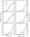 |
Fig. 2. Charge-state distribution of C plasma at electron temperatures and densities of 120 eV and 4.30 × 1022 cm−3 (a), 189 eV and 8.70 × 1022 cm−3 (b), 251 eV and 2.06 × 1023 cm−3 (c), 303 eV and 4.32 × 1023 cm−3 (d), 373 eV and 1.06 × 1024 cm−3 (e), and 496 eV and 3.51 × 1024 cm−3 (f). These plasma conditions are deduced from the standard solar model (Bahcall & Ulrich 1988; Guenther et al. 1992) at radius fractions of 0.796 R⊙, 0.7133 R⊙, 0.6195 R⊙, 0.5442 R⊙, 0.4597 R⊙, and 0.3529 R⊙, respectively. Our results are compared with those of the Debye–Hückel (DH; Debye & Hückel 1923), Stewart–Pyatt (SP; Stewart & Pyatt 1966), ion-sphere (IS; Rozsnyai 1972), and Ecker–Kröll (EK; Ecker & Kröll 1963) analytical models. |
3.2. Carbon plasma under stellar interior conditions
In stellar interiors, plasma conditions can vary over a wide temperature range (up to several keV) and a mass-density range (up to several thousands of g cm−3) (Chabrier & Baraffe 2000). Subsequently, we constrained our case studies below a temperature and mass density of 500 eV and 10 g cm−3, respectively. These plasma conditions also exist in inertial confinement fusion experiments (Hurricane 2014) and are meaningful for interpreting the experiments (Kraus et al. 2016, 2019).
Figure 3 shows the IPDs of C plasma at temperatures of 200 and 400 eV and mass densities of 2.25, 3.75, and 5.0 g cm−3. The dependence of the predicted IPDs on different theoretical models shows different features, as discussed above under solar interior conditions. The best overall agreement is obtained with the IS model (Rozsnyai 1972), particularly at densities higher than 3.75 g cm−3. Under these circumstances, the IS model captures the essential features at a high-density limit in the case of C plasma. The second-best agreement is found with the prediction of the SP model (Stewart & Pyatt 1966), which obtains smaller IPDs than our theoretical results. The Ecker–Kröll model (Ecker & Kröll 1963) always predicted the highest IPDs; however, the IPDs obtained using the Debye–Hückel model (Debye & Hückel 1923) were considerably lower than our theoretical results. The discrepancies between the Debye–Hückel model and our model increase with an increasing temperature and density.
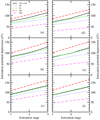 |
Fig. 3. Ionization potential depressions of C plasma at a temperature of 200 eV and mass densities of 2.25 g cm−3 (a), 3.75 g cm−3 (b), and 5.0 g cm−3 (c) and at a temperature of 400 eV and mass densities of 2.25 g cm−3 (d), 3.75 g cm−3 (e), and 5.0 g cm−3 (f). Our results are compared with the Debye–Hückel (DH; Debye & Hückel 1923), Stewart–Pyatt (SP; Stewart & Pyatt 1966), ion-sphere (IS; Rozsnyai 1972), and Ecker–Kröll (EK; Ecker & Kröll 1963) analytical models. |
In Fig. 4, we compare the CSDs of C4+, C5+, and bare-ion C6+ obtained herein with those of the analytical models. The CSDs are shown as a function of the plasma temperature at mass densities of 2.25, 3.75, and 5.0 g cm−3. At a mass density of 2.25 g cm−3, the population fractions of different ionization stages predicted by our model are in reasonable agreement with those of the SP (Stewart & Pyatt 1966) and IS (Rozsnyai 1972) models, whereas large discrepancies are found with the Ecker–Kröll (Ecker & Kröll 1963) and Debye–Hückel (Debye & Hückel 1923) models. The reasonable agreement of our predicted CSDs with those of the SP and IS models indicates the consistency of the predicted IPDs of this theory, as demonstrated in Fig. 3. The Debye–Hückel model is not applicable to such dense plasma, where the CSDs are predicted toward the lower ionization stages. The unreasonable prediction of the Debye–Hückel model abruptly increases the population fraction of C5+ and decreases that of C6+. However, the Ecker–Kröll model (Ecker & Kröll 1963) predicts a much higher population fraction of C6+ compared with that obtained using our model. This differs from the conclusion drawn using the solid-density Mg, Al, and Si plasma (Ciricosta et al. 2012, 2016; Zeng et al. 2020), where the IPDs determined by the Ecker–Kröll model were in much better agreement with the experimental results than those of the SP model.
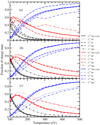 |
Fig. 4. Charge-state distribution of C plasma as a function of the plasma temperature at mass densities of 2.25 g cm−3 (a), 3.75 g cm−3 (b), and 5.0 g cm−3 (c). Our results are compared with the Debye–Hückel (DH; Debye & Hückel 1923), Stewart–Pyatt (SP; Stewart & Pyatt 1966), ion-sphere (IS; Rozsnyai 1972), and Ecker–Kröll (EK; Ecker & Kröll 1963) analytical models. |
We obtained the best agreement with the Ecker–Kröll model (Ecker & Kröll 1963) for the CSDs at a mass density of 3.75 g cm−3. The SP (Stewart & Pyatt 1966), IS (Rozsnyai 1972), and Debye-Hückel (Debye & Hückel 1923) models predicted a higher population fraction for C5+ and a lower fraction for C6+ than those predicted by our model and the Ecker–Kröll model. With the increasing mass density up to 5.0 g cm−3, our theoretical IPDs and those of the IS and Ecker–Kröll models exhibited good agreement. The SP and Debye–Hückel models predicted a higher population fraction for C5+ and a lower fraction for C6+.
The aforementioned results can be seen in Fig. 5, which shows the average ionization degree of C plasma as a function of the plasma temperature (100–500 eV) at mass densities of 2.25, 3.75, and 5.0 g cm−3. Our predicted average ionization degree is consistent with those of the Ecker–Kröll model (Ecker & Kröll 1963) at a density of 3.75 g cm−3 and the IS and Ecker–Kröll models at a density of 5.0 g cm−3, which is completely in accordance with the features observed with respect to CSDs (Fig. 4).
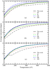 |
Fig. 5. Average ionization degree of C plasma as a function of plasma temperature at mass densities of 2.25 g cm−3 (a), 3.75 g cm−3 (b), and 5.0 g cm−3 (c). Our results are compared with the Debye–Hückel (Debye & Hückel 1923), Stewart–Pyatt (Stewart & Pyatt 1966), ion-sphere (Rozsnyai 1972), and Ecker–Kröll (Ecker & Kröll 1963) analytical models. |
3.3. Analysis and explanation of a recent experiment
Here, we verify the validity of our proposed model of screening potential by comparing its predictions with the results of a recent experimental measurement of the average ionization degree of C in a CH-mixture plasma (Kraus et al. 2016). In this experiment, a highly compressed CH-mixture plasma (polystyrene) was created via spherically convergent shocks at the National Ignition Facility. Then, the spectrally resolved X-ray scattering of line radiation at 9.0 keV was recorded. The experiment measured an average ionization degree of 4.92 ± 0.15 for C at an average temperature of 86 ± 20 eV (radiation–hydrodynamics simulations show that the temperature varies during the shocks) and a density of 6.74 g cm−3.
Figure 6 shows our theoretical average ionization degree of C in a CH-mixture plasma as a function of the temperature in comparison with the SP (Stewart & Pyatt 1966) and Thomas–Fermi (TF; More et al. 1988) predictions at mass densities of 3.0, 5.0, 6.74, and 9.0 g cm−3 (Kraus et al. 2016). The only experimental result and the error bars of the temperature and density are shown in the plot to evaluate the theoretical models. From the comparison in Fig. 6, our calculated average ionization degree of C is much closer to the experimental result (Kraus et al. 2016) than to the predictions of the SP (Stewart & Pyatt 1966) and TF (More et al. 1988) models. From Figs. 3–5, the widely used SP model predicted a lower average ionization degree than our model. Our predicted average ionization degree of C agrees with the experimentally obtained result within the error bar of the temperature and density (Kraus et al. 2016) at a mass density of 6.74 g cm−3. The average ionization degree is predicted to be 4.86, which falls within the experimental value of 4.92 ± 0.15 at a temperature of 106 eV, which is the higher limit of the error bar for 86 ± 20 eV. The free electrons contributed by the hydrogen atoms play a role in the determination of the average ionization degree of C, and its effect has been included. The contribution of free electrons from the hydrogen atoms to the IPDs of C can be seen in Fig. 7.
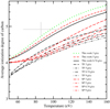 |
Fig. 6. Comparison of the average ionization degree of C in a CH-mixture plasma obtained herein with the experimental and theoretical predictions obtained by the Stewart–Pyatt (SP) and Thomas–Fermi (TF) models at various plasma conditions (Kraus et al. 2016). The average ionization degree is given as a function of the plasma temperature at mass densities of 3.0 g cm−3, 5.0 g cm−3, 6.74 g cm−3, and 9.0 g cm−3. |
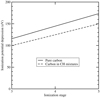 |
Fig. 7. Ionization potential depressions of pure C and CH-mixture plasma at a temperature of 100 eV and a mass density of 6.74 g cm−3 of the CH mixture, which corresponds to 6.2 g cm−3 for pure C plasma. |
The ionization competition effect (Li et al. 2015) between C and H is considered in the solution of the Saha equation for the CH-mixture plasma. Practical calculations indicate that this effect is small in the experimental sample (Kraus et al. 2016) and under the given plasma conditions; however, the screening of C ions contributed by the free electrons of H atoms must be considered.
4. Summary and conclusions
Herein, we investigate the effect of the plasma screening potential on the shifts in the energy levels and IPDs of the ions embedded in dense C plasma under solar and stellar interior conditions using our recently developed consistent nonanalytical model. We then focus on the screening effect on ionization balance using our model and the SP, IS, Ecker–Kröll, and Debye–Hückel analytical models. Under the solar interior conditions, our IPD and CSD were close to those of the Ecker–Kröll model below the electron temperature and density of 303 eV and 4.32 × 1023 cm−3. At 373 eV and 1.06 × 1024 cm−3, better agreement is found with the IS model. This difference increases with the increasing temperature and density. The Debye–Hückel model underestimates the IPD and average ionization degree. For dense C plasma with mass densities of 2.25–5.0 g cm−3, the IPD, CSD, and average ionization degree predicted by our model are in better agreement with the IS model than the SP model. The widely used SP model underestimates the IPD and average ionization degree, whereas the Ecker–Kröll model overestimates them. Our theoretical model is further validated by comparing the predicted average ionization degree of C in a dense CH-mixture plasma with the experimental results. The results demonstrate that our plasma screening model provides an accurate description of the IPD and ionization balance in solar and stellar interiors and can be used to provide more accurate equations of state and opacity as inputs for the standard solar model.
Accurate IPD and ionization balance models that consider CSDs and the average ionization degree are important to investigate the equations of state and opacity. When using the updated opacities, a persistent inconsistency remains between the internal solar structure predicted by the standard solar model and the results of helioseismic studies (Basu & Antia 2008; Serenelli et al. 2009; Bahcall et al. 2004). This has brought about renewed interest in obtaining more accurate opacity (Bailey et al. 2015). Ionization balance with a better description of IPDs is expected to be one of the major factors in improving the accuracy of opacity and equations of state in solar and stellar interiors.
Acknowledgments
This work was supported by Science Challenge Project No. TZ2018005, by the National Key R&D Program of China under the grant No. 2019YFA0307700 and No. 2017YFA0403202, and by the National Natural Science Foundation of China under Grant Nos. 11674394.
References
- Ali, A., Naz, G. S., Shahzad, M. S., et al. 2018, High Energy Density Phys., 26, 48 [NASA ADS] [CrossRef] [Google Scholar]
- Andrea, L., Swift, D. C., Glenzer, S. H., et al. 2020, Nature, 584, 51 [CrossRef] [Google Scholar]
- Bahcall, J. N., & Ulrich, R. K. 1988, Rev. Mod. Phys., 60, 297 [NASA ADS] [CrossRef] [Google Scholar]
- Bahcall, J. N., Serenelli, A. M., & Pinsonneault, M. 2004, ApJ, 614, 464 [NASA ADS] [CrossRef] [Google Scholar]
- Bailey, J. E., Nagayama, T., Loisel, G. P., et al. 2015, Nature, 517, 56 [NASA ADS] [CrossRef] [Google Scholar]
- Basu, S., & Antia, H. M. 2008, Phys. Rep., 457, 217 [NASA ADS] [CrossRef] [Google Scholar]
- Calisti, A., Ferri, S., & Talin, B. 2015, J. Phys. B: At. Mol. Opt. Phys., 48, 224003 [NASA ADS] [CrossRef] [Google Scholar]
- Chabrier, G., & Baraffe, I. 2000, ARA&A, 38, 337 [NASA ADS] [CrossRef] [Google Scholar]
- Ciricosta, O., Vinko, S. M., Chung, H.-K., et al. 2012, Phys. Rev. Lett., 109, 065002 [NASA ADS] [CrossRef] [PubMed] [Google Scholar]
- Ciricosta, O., Vinko, S. M., Barbrel, B., et al. 2016, Nat. Commun., 7, 11713 [NASA ADS] [CrossRef] [Google Scholar]
- Crowley, B. J. B. 2014, High Energy Density Phys., 13, 84 [NASA ADS] [CrossRef] [Google Scholar]
- Debye, P., & Hückel, E. 1923, Phys. Z., 24, 185 [Google Scholar]
- Dharma-Wardana, M. W. C., & Taylor, R. 1981, J Phys. C: Solid State Phys., 14, 629 [NASA ADS] [CrossRef] [Google Scholar]
- Dufour, P., Liebert, J., Fontaine, G., & Behara, N. 2007, Nature, 450, 522 [NASA ADS] [CrossRef] [PubMed] [Google Scholar]
- Ecker, G., & Kröll, W. 1963, Phys. Fluids, 6, 62 [NASA ADS] [CrossRef] [Google Scholar]
- Fletcher, L. B., Kritcher, A. L., Pak, A., et al. 2014, Phys. Rev. Lett., 112, 145004 [NASA ADS] [CrossRef] [Google Scholar]
- Fontaine, G., & Van Horn, H. M. 1976, ApJS, 31, 467 [NASA ADS] [CrossRef] [Google Scholar]
- Gao, C., Zeng, J. L., & Yuan, J. M. 2011, High Energy Density Phys., 7, 54 [NASA ADS] [CrossRef] [Google Scholar]
- Gao, C., Zeng, J. L., Li, Y. Q., Jin, F. T., & Yuan, J. M. 2013, High Energy Density Phys., 9, 583 [NASA ADS] [CrossRef] [Google Scholar]
- Guenther, D. B., Demarque, P., Kim, Y.-C., & Pinsonneault, M. H. 1992, ApJ, 387, 372 [NASA ADS] [CrossRef] [Google Scholar]
- Gu, M. F. 2008, Can. J. Phys., 86, 675 [NASA ADS] [CrossRef] [Google Scholar]
- Hansen, S. B., Colgan, J., Faenov, A. Ya, et al. 2014, Phys. Plasmas, 21, 031213 [NASA ADS] [CrossRef] [Google Scholar]
- Hoarty, D. J., Allan, P., James, S. F., et al. 2013, Phys. Rev. Lett., 110, 265003 [NASA ADS] [CrossRef] [PubMed] [Google Scholar]
- Hu, S. X. 2017, Phys. Rev. Lett., 119, 065001 [NASA ADS] [CrossRef] [Google Scholar]
- Hurricane, O. A., et al. 2014, Nature, 506, 343 [CrossRef] [PubMed] [Google Scholar]
- Iglesias, C. A. 2014, High Energy Density Phys., 12, 5 [NASA ADS] [CrossRef] [Google Scholar]
- Kasim, M. F., Wark, J. S., & Vinko, S. M. 2018, Sci. Rep., 8, 6276 [NASA ADS] [CrossRef] [Google Scholar]
- Kramida, A., Ralchenko, Y., & Reader, J., NIST ASD Team 2020, Available at: https://physics.nist.gov/asd [2020, May 8] [Google Scholar]
- Kraus, D., Chapman, D. A., Kritcher, A. L., et al. 2016, Phys. Rev. E, 94, 011202(R) [CrossRef] [Google Scholar]
- Kraus, D., Bachmann, B., Barbrel, B., et al. 2019, Plasma Phys. Control. Fusion, 61, 014015 [NASA ADS] [CrossRef] [Google Scholar]
- Li, Y. Q., Wu, J. H., Hou, Y., & Yuan, J. M. 2008, J. Phys. B: At. Mol. Opt. Phys., 41, 145002 [NASA ADS] [CrossRef] [Google Scholar]
- Li, Y. J., Gao, C., Tian, Q. Y., Zeng, J. L., & Yuan, J. M. 2015, Phys. of Plasma, 22, 113302 [CrossRef] [Google Scholar]
- Lin, C. L. 2019, Phys. Plasmas, 26, 122707 [CrossRef] [Google Scholar]
- Lin, C. L., Röpke, G., Kraeft, W. D., & Reinholz, H. 2017, Phys. Rev. E, 96, 013202 [NASA ADS] [CrossRef] [Google Scholar]
- More, R. M., Warren, K. H., Young, D. A., & Zimmerman, G. B. 1988, Phys. Fluids, 31, 3059 [NASA ADS] [CrossRef] [Google Scholar]
- Preston, T. R., Vinko, S. M., Ciricosta, O., et al. 2013, High Energy Density Phys., 9, 258 [NASA ADS] [CrossRef] [Google Scholar]
- Röpke, G., Blaschke, D., Döppner, T., et al. 2019, Phys. Rev. E, 99, 033201 [NASA ADS] [CrossRef] [Google Scholar]
- Rosmej, F. B. 2018, J. Phys. B: At. Mol. Opt. Phys., 51, 09LT01 [CrossRef] [Google Scholar]
- Rozsnyai, B. F. 1972, Phys. Rev. A, 5, 1137 [NASA ADS] [CrossRef] [Google Scholar]
- Seddon, E. A., Clarke, J. A., Dunning, D. J., et al. 2017, Rep. Prog. Phys., 80, 115901 [CrossRef] [Google Scholar]
- Serenelli, A. M., Basu, S., Ferguson, J. W., & Asplund, M. 2009, ApJ, 705, L123 [NASA ADS] [CrossRef] [Google Scholar]
- Son, S.-K., Thiele, R., Jurek, Z., Ziaja, B., & Santra, R. 2014, Phys. Rev. X, 4, 031004 [Google Scholar]
- Stewart, J. C., & Pyatt, K. D., Jr 1966, ApJ, 144, 1203 [NASA ADS] [CrossRef] [Google Scholar]
- Stransky, M. 2016, Phys. Plasmas, 23, 012708 [NASA ADS] [CrossRef] [Google Scholar]
- Vinko, S. M., Ciricosta, O., & Wark, J. S. 2014, Nat. Commun., 5, 3533 [NASA ADS] [CrossRef] [Google Scholar]
- Yuan, J. M. 2002, Phys. Rev. E, 66, 047401 [NASA ADS] [CrossRef] [Google Scholar]
- Zeng, J. L., Li, Y. J., Gao, C., & Yuan, J. M. 2020, A&A, 634, A117 [CrossRef] [EDP Sciences] [Google Scholar]
All Tables
Level energies and ionization potential (IP; in eV) for the isolated atom (IA) and screened atom of C4+ embedded in C plasmas at an electron temperature and density of 120 eV and 4.3 × 1022 cm−3 (A), 189 eV and 8.7 × 1022 cm−3 (B), 250 eV and 2.1 × 1023 cm−3 (C), 303 eV and 4.3 × 1023 cm−3 (D), and 373 eV and 1.1 × 1024 cm−3 (E).
Level energies and ionization potential (IP; in eV) for the isolated atom (IA) and screened atom of C5+ embedded in carbon plasmas at an electron temperature and density of 120 eV and 4.3 × 1022 cm−3 (A), 189 eV and 8.7 × 1022 cm−3 (B), 250 eV and 2.1 × 1023 cm−3 (C), 303 eV and 4.3 × 1023 cm−3 (D), and 373 eV and 1.1 × 1024 cm−3 (E).
All Figures
|
Fig. 1. Ionization potential depressions of C plasma at electron temperatures and densities of 120 eV and 4.30 × 1022 cm−3 (a), 189.00 eV and 8.70 × 1022 cm−3 (b), 251 eV and 2.06 × 1023 cm−3 (c), 303 eV and 4.32 × 1023 cm−3 (d), 373 eV and 1.06 × 1024 cm−3 (e), and 496 eV and 3.51 × 1024 cm−3 (f). These plasma conditions are deduced from the standard solar model (Bahcall & Ulrich 1988; Guenther et al. 1992) at radius fractions of 0.796 R⊙, 0.7133 R⊙, 0.6195 R⊙, 0.5442 R⊙, 0.4597 R⊙, and 0.3529 R⊙, respectively. Our results are compared with those of the Debye–Hückel (DH; Debye & Hückel 1923), Stewart–Pyatt (SP; Stewart & Pyatt 1966), ion-sphere (IS; Rozsnyai 1972), and Ecker–Kröll (EK; Ecker & Kröll 1963) analytical models. The description of the line style shown in plot (a) applies to all plots (a)–(f). |
| In the text | |
|
Fig. 2. Charge-state distribution of C plasma at electron temperatures and densities of 120 eV and 4.30 × 1022 cm−3 (a), 189 eV and 8.70 × 1022 cm−3 (b), 251 eV and 2.06 × 1023 cm−3 (c), 303 eV and 4.32 × 1023 cm−3 (d), 373 eV and 1.06 × 1024 cm−3 (e), and 496 eV and 3.51 × 1024 cm−3 (f). These plasma conditions are deduced from the standard solar model (Bahcall & Ulrich 1988; Guenther et al. 1992) at radius fractions of 0.796 R⊙, 0.7133 R⊙, 0.6195 R⊙, 0.5442 R⊙, 0.4597 R⊙, and 0.3529 R⊙, respectively. Our results are compared with those of the Debye–Hückel (DH; Debye & Hückel 1923), Stewart–Pyatt (SP; Stewart & Pyatt 1966), ion-sphere (IS; Rozsnyai 1972), and Ecker–Kröll (EK; Ecker & Kröll 1963) analytical models. |
| In the text | |
|
Fig. 3. Ionization potential depressions of C plasma at a temperature of 200 eV and mass densities of 2.25 g cm−3 (a), 3.75 g cm−3 (b), and 5.0 g cm−3 (c) and at a temperature of 400 eV and mass densities of 2.25 g cm−3 (d), 3.75 g cm−3 (e), and 5.0 g cm−3 (f). Our results are compared with the Debye–Hückel (DH; Debye & Hückel 1923), Stewart–Pyatt (SP; Stewart & Pyatt 1966), ion-sphere (IS; Rozsnyai 1972), and Ecker–Kröll (EK; Ecker & Kröll 1963) analytical models. |
| In the text | |
|
Fig. 4. Charge-state distribution of C plasma as a function of the plasma temperature at mass densities of 2.25 g cm−3 (a), 3.75 g cm−3 (b), and 5.0 g cm−3 (c). Our results are compared with the Debye–Hückel (DH; Debye & Hückel 1923), Stewart–Pyatt (SP; Stewart & Pyatt 1966), ion-sphere (IS; Rozsnyai 1972), and Ecker–Kröll (EK; Ecker & Kröll 1963) analytical models. |
| In the text | |
|
Fig. 5. Average ionization degree of C plasma as a function of plasma temperature at mass densities of 2.25 g cm−3 (a), 3.75 g cm−3 (b), and 5.0 g cm−3 (c). Our results are compared with the Debye–Hückel (Debye & Hückel 1923), Stewart–Pyatt (Stewart & Pyatt 1966), ion-sphere (Rozsnyai 1972), and Ecker–Kröll (Ecker & Kröll 1963) analytical models. |
| In the text | |
|
Fig. 6. Comparison of the average ionization degree of C in a CH-mixture plasma obtained herein with the experimental and theoretical predictions obtained by the Stewart–Pyatt (SP) and Thomas–Fermi (TF) models at various plasma conditions (Kraus et al. 2016). The average ionization degree is given as a function of the plasma temperature at mass densities of 3.0 g cm−3, 5.0 g cm−3, 6.74 g cm−3, and 9.0 g cm−3. |
| In the text | |
|
Fig. 7. Ionization potential depressions of pure C and CH-mixture plasma at a temperature of 100 eV and a mass density of 6.74 g cm−3 of the CH mixture, which corresponds to 6.2 g cm−3 for pure C plasma. |
| In the text | |
Current usage metrics show cumulative count of Article Views (full-text article views including HTML views, PDF and ePub downloads, according to the available data) and Abstracts Views on Vision4Press platform.
Data correspond to usage on the plateform after 2015. The current usage metrics is available 48-96 hours after online publication and is updated daily on week days.
Initial download of the metrics may take a while.