| Issue |
A&A
Volume 644, December 2020
|
|
|---|---|---|
| Article Number | A164 | |
| Number of page(s) | 13 | |
| Section | Extragalactic astronomy | |
| DOI | https://doi.org/10.1051/0004-6361/202038550 | |
| Published online | 15 December 2020 | |
Shedding light on the formation mechanism of shell galaxy NGC 474 with MUSE⋆
1
Univ. Lyon, ENS de Lyon, Univ. Lyon 1, CNRS, Centre de Recherche Astrophysique de Lyon, UMR5574, 69007 Lyon, France
e-mail: This email address is being protected from spambots. You need JavaScript enabled to view it.
2
European Southern Observatory, Karl-Schwarzschild-Str. 2, 85748 Garching, Germany
3
Observatoire Astronomique de Strasbourg (ObAS), Université de Strasbourg – CNRS, UMR7550, Strasbourg, France
4
University of Tampa, 401 West Kennedy Boulevard, Tampa, FL 33606, USA
5
Univ. Lyon, Univ. Lyon 1, ENS de Lyon, CNRS, Centre de Recherche Astrophysique de Lyon, UMR5574, 69230 Saint-Genis-Laval, France
6
Department of Physics & Astronomy, Youngstown State University, Youngstown, OH 44555, USA
7
Department of Astronomy, School of Physics and Astronomy, and Shanghai Key Laboratory for Particle Physics and Cosmology, Shanghai Jiao Tong University, Shanghai 200240, PR China
8
Department of Astronomy, Peking University, Yi He Yuan Lu 5, Hai Dian District, Beijing 100871, PR China
9
Kavli Institute for Astronomy & Astrophysics and Department of Astronomy, Peking University, Yi He Yuan Lu 5, Hai Dian District, Beijing 100871, PR China
10
Korea Astronomy and Space Science Institute (KASI), 776 Daedeokdae-ro, Yuseong-gu, Daejeon 34055, Korea
Received:
1
June
2020
Accepted:
4
November
2020
Abstract
Stellar shells around galaxies could provide precious insights into their assembly history. However, their formation mechanism remains poorly empirically constrained, regarding in particular the type of galaxy collisions at their origin. We present MUSE at VLT data of the most prominent outer shell of NGC 474, to constrain its formation history. The stellar shell spectrum is clearly detected, with a signal-to-noise ratio of ∼65 pix−1. We used a full spectral fitting method to determine the line-of-sight velocity and the age and metallicity of the shell and associated point-like sources within the MUSE field of view. We detect six globular cluster (GC) candidates and eight planetary nebula (PN) candidates that are all kinematically associated with the stellar shell. We show that the shell has an intermediate metallicity, [M/H] = −0.83−0.12+0.12, and a possible α-enrichment, [α/Fe] ∼ 0.3. Assuming the material of the shell comes from a lower mass companion, and that the latter had no initial metallicity gradient, such a stellar metallicity would constrain the mass of the progenitor at around 7.4 × 10⁸ M⊙, implying a merger mass ratio of about 1:100. However, our census of PNe and earlier photometry of the shell would suggest a much higher ratio, around 1:20. Given the uncertainties, this difference is only significant at the ≃1σ level. We discuss the characteristics of the progenitor, and in particular whether the progenitor could also be composed of stars from the low-metallicity outskirts of a more massive galaxy. Ultimately, the presented data do not allow us to put a firm constraint on the progenitor mass. We show that at least two GC candidates possibly associated with the shell are quite young, with ages below 1.5 Gyr. We also note the presence of a young (∼1 Gyr) stellar population in the center of NGC 474. The two may have resulted from the same event.
Key words: galaxies: interactions / galaxies: peculiar / galaxies: star clusters: general / galaxies: halos
Based on data from ESO program 099.B-0328(A) (PI: Fensch).
© J. Fensch et al. 2020
 Open Access article, published by EDP Sciences, under the terms of the Creative Commons Attribution License (https://creativecommons.org/licenses/by/4.0), which permits unrestricted use, distribution, and reproduction in any medium, provided the original work is properly cited.
1. Introduction
According to the current cosmological paradigm, galaxies assemble through a continuous process of accretion of gas and successive merging with other galaxies (White & Rees 1978). This merging history can leave low surface brightness (LSB) imprints in the halo of a galaxy, and in the shape of stellar streams, plumes, tidal tails, or shells (see e.g., Mihos et al. 2005; Martínez-Delgado et al. 2010; van Dokkum et al. 2014; Duc et al. 2015; Mancillas et al. 2019a; Müller et al. 2019). Thus, the study of these features can help to reconstruct the assembly histories of galaxies (see e.g., Foster et al. 2014; Longobardi et al. 2015), as well as serving as probes for gravity in the low-acceleration regime (see e.g., Ebrová et al. 2012; Bílek et al. 2013).
Young prominent tidal tails are mostly gas rich and can be analyzed through their gas component (see e.g., Yun et al. 1994; Duc et al. 2000; Williams et al. 2002). However, plumes, streams, and shells are relatively gas poor (however, see Charmandaris et al. 2000), and only their faint stellar absorption lines are usually available for spectroscopy. An alternative when studying the dynamics and chemical composition of gas-poor tidal features is to use bright point sources, such as globular clusters (GC) or planetary nebulae (PNe) to study the dynamics and chemical composition of plumes or streams (see e.g., Durrell et al. 2003; Mullan et al. 2011; Forbes et al. 2012; Blom et al. 2014; Foster et al. 2014).
Stellar shells are relatively frequent around elliptical and lenticular galaxies (∼20%, Tal et al. 2009; Duc et al. 2015; Pop et al. 2018, but see Krajnović et al. 2011) and have relatively high surface brightness for LSB structures (up to 25 mag arcsec−2; Johnston et al. 2008; Atkinson et al. 2013) compared to streams and plumes. They thus appear as convenient tracers of past merging events. Shell systems have been classified under three types, corresponding to the distribution of the shells’ position angles: Type I for aligned shells, Type II for random orientation, and Type III for ambiguous or undetermined orientations (Wilkinson et al. 1987).
From numerical simulations, it could be inferred that the mechanisms responsible for shell formation are likely to be near-radial infalls of relatively massive galaxies (mass ratio above 1:10; see e.g., Quinn 1984; Hernquist & Spergel 1992; Pop et al. 2018; Karademir et al. 2019), while mergers involving higher angular momentum tend to create stellar streams (Amorisco 2015; Hendel & Johnston 2015). It should be noted that high mass ratios are favored, as higher mass progenitors should be able to create shells from a wider range of impact parameters (Pop et al. 2018). Shells are therefore thought to be made up of stars from the accreted and tidally disrupted satellite, at the apocenter of their orbit around the host galaxy. However, the spectrophotometric data needed to test these scenarios are scarce, mostly because they are extremely challenging to obtain (however, see longslit spectra from Pence 1986). Moreover, this paucity means that the extent to which point sources – namely GCs and PNe – could trace the kinematics of these stellar structures is still unknown.
In this study, we propose to empirically constrain the formation scenario of stellar shells by using the revolutionary capabilities of MUSE on one of the most spectacular shell-rich systems, NGC 474. This galaxy, classified as peculiar by Arp (1966) under the name Arp 227, is either a lenticular galaxy or a fast rotating elliptical (Hau et al. 1996; Emsellem et al. 2004), located at 30.9 Mpc (Cappellari et al. 2011). The deepest imaging data obtained to date on this system revealed a total of at least ten concentric shells and six radial streams up to 5.6′ from the galaxy (i.e., 50 kpc; Duc et al. 2015, MATLAS survey). The nonalignment of the position angles of the inner shells around the galaxy (within 100″, i.e., 15 kpc from the center) classified NGC 474 as a Type II shell galaxy (Prieur 1990; Turnbull et al. 1999). These inner shell systems have already been studied via their photometry (Sikkema et al. 2006, 2007), which revealed the presence of a blue inner shell, giving a hint of a recent minor merger event. In this paper, we present the data obtained on the brightest shell (24.8 mag arcsec−2 in the g-band), located ∼30 kpc away from the host, which has a few spatially associated GC candidates, selected by color on ultra-deep CFHT imaging (Lim et al. 2017; L17 in the following).
The paper is organized as follows. The data and methods are presented in Sect. 2 and the results in Sect. 3. The discussion and conclusion are presented in Sects. 4 and 5. All magnitudes are AB magnitudes.
2. Data and methods
2.1. Observations and reduction steps
The VLT/MUSE observations were conducted in service mode during gray time from November 2017 to November 2018, with CLEAR conditions and observed seeing between 0.5″ and 0.9″. Observations were split into 16 observing blocks (OBs) of one hour each, amounting to a total 5.1 h on-target integration time for each of the two pointings. Each OB was split into four individual on-target exposures with small dithers and 90° rotations to avoid cosmic ray contamination and slicer patterns. All OBs had an “OSOOSO” sequence, where S stands for sky, with each 150 s exposure, and O stands for object, for each 583 s exposure. Figure 1 shows the location of the field of view. We overlapped the two pointing footprints to increase the signal-to-noise on the shell.
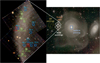 |
Fig. 1. Left: true color image constructed from the MUSE data using the g, r, and i filters of Megacam at CFHT as colors. The locations of the detected PNe are shown with blue circles. In green, we show the detected GCs. GCs 4, 5, and 6 were part of the L17 sample: their number in that catalog is given after their name. The two red circles show detections that were classified by L17 as GC candidates but are not confirmed with the present data. Right: zoom-out true-color image from CFHT (g, r, i bands from Duc et al. 2015). The MUSE and SKY pointings are shown, respectively, in white and yellow. The SAURON pointing from de Zeeuw et al. (2002) is shown in blue. The MUSE and SAURON pointings are, respectively, 1′×1′ and 33″ × 41″ wide. Assuming a distance to NGC 474 of 30.9 Mpc (Cappellari et al. 2011), 1′ encompasses around 8.9 kpc. North is up and west is right. |
The OBs were all reduced using the latest MUSE ESOREX pipeline recipes (version 2.4.2 from Weilbacher et al. 2020). The reduction follows the standard steps, including sky subtraction. To improve sky subtraction, we used the Zurich Atmosphere Purge software (ZAP; Soto et al. 2016), and the sky available on the left of the shell. We used 45 eigenvectors and 300 pixels for the window for the continuum subtraction.
In Fig. 1, we also show the field of view of archival1 SAURON data centered on NGC 474 (de Zeeuw et al. 2002; Cappellari et al. 2011). This data is discussed in Sect. 4.2.
2.2. Detection and spectral extraction
We detected GCs and PNe using SExtractor on collapsed cubes (Bertin & Arnouts 1996). GC detections were done on the fully collapsed cube. We selected well-defined, point-like detections that had a velocity consistent with being part of this system, that is ±400 km s−1 around the central velocity of NGC 474 and a signal to noise ratio (S/N) above 6 pix−1, plus the candidates from L17. PNe were detected on a stack image of two collapsed cubes, each using only frames (slabs of 7.5 Å) around the redshifted wavelengths of each of the [O III] doublet emission line. To remove the continuum we constructed a second image from two similarly collapsed cubes from nearby, but featureless, spectral regions, and we subtracted this image from the first image. Eight sources with unambiguous detection of the [O III] doublet (S/N > 2.5) were detected, their location is indicated in Fig. 1.
We extracted each point source with a Gaussian weight function to provide an S/N-optimised extraction. The full width at half maximum is chosen to be ∼0.8″ to approximately match the resulting point spread function. The background is measured locally in eight locations, using the same Gaussian weight. In each channel, we subtracted the median value of background regions to the source flux. The variance between those eight sky apertures is added to the source flux variance channel per channel. The flux from the shell is obtained by a sum of the flux on the full shell, after masking point sources, weighted by the white-light image to optimize the S/N.
The best single stellar population (SSP) fit for the shell and the brightest GC (GC 2) are shown in Fig. 2. The gray regions are affected by residual sky lines and were not used for the fit. The other fits are presented in the appendix, and the methods are described in the next subsection. We note strong Balmer and calcium triplet (CaT) absorption lines, but no emission lines. The S/N around the Hα line is 65 pix−1 for the shell, 26.9 pix−1 for GC 2, and 6.6 pix−1 for GC 3, respectively. The PNe candidate spectra are shown in Fig. 3. The S/N goes from 9.1 for PN 6 to 4.5 for PN 4.
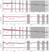 |
Fig. 2. Comparison between spectrum and best SSP fit from pPXF for the shell and GC 2. The three plots in the bottom part of each panel show zooms of the important absorption lines. The gray regions are not taken into account for the fit. The scatter points show the residuals. |
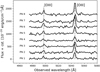 |
Fig. 3. Spectra of the eight PNe candidates. The location of the [OIII] doublet at the redshift of NGC 474 is shown with gray dashed lines. |
3. Results
3.1. Full spectral analysis
The method used is the same as the one described in Fensch et al. (2019). It is mainly based on pPXF (Cappellari 2017) and the eMILES single stellar population (SSP) library (Vazdekis et al. 2016). We linearly interpolate for sixteen more metallicity values, between [Fe/H] = −2.32 and −0.71, as was done in Kuntschner et al. (2010). In the following, we summarize the main points of the procedure.
For the shell and the GC candidates, we used pPXF with Legendre polynomials to account for uncertainty in the different flux calibrations between our data and the eMILES library. For the kinematic fits, we used 12° multiplicative and 14° additive Legendre polynomials, and the full eMILES library, similarly to Emsellem et al. (2019). For the stellar population fits, we used 12° multiplicative and no additive Legendre polynomials, and we individually fit the input spectrum with each SSP, as in Fensch et al. (2019). The ages we derived were then those of the best-fit single burst of star formation. Uncertainty on the results is obtained from a bootstrap method, consisting of resampling the residuals. This assumes that the residuals from the best fit are a good representation of the overall noise of the spectrum, which is a reasonable assumption given the very small dependance of the residual spread with the wavelength seen in Fig. 2. We randomly redistributed the residuals from the best fit to obtain a residual spectrum, which we added to the best fit to create a re-noised spectrum. We repeated the operation 100 times to get a 100 re-noised spectra, and the uncertainty is obtained as the dispersion in the new best-fit value for the 100 new fits. For the PNe, we used a double Gaussian line emission template with the same width to fit the [OIII] doublet. The uncertainty was obtained in the same way as for the shell and GCs.
The result of the kinematic fits is shown in Fig. 4. The GC and PN candidates measured velocities within 50 km s−1 of the shell’s velocity, as determined from the integrated MUSE spectrum. This kinematical association thus confirms a plausible association between them and the stellar shell. One should keep in mind that the velocity profile of a stellar shell is expected to present a four-horn profile with a wide separation between the extreme values (up to 150 km s−1; see e.g., Ebrová et al. 2012). A spread of velocities of the PNe and GCs around the velocity of the integrated shell spectra is thus expected for such systems. We further note that the shell velocity, 2307.6 ± 2.7 km s−1, is similar to that of the central regions of NGC 474 (2315 ± 5 km s−1Cappellari et al. 2011). This fits with the interpretation that the shell is made of stars originating from the disrupted satellite that just reach the apocenter of their orbits in the potential well of the host galaxy. The sharp contrast of the shell emerges from a favorable projection, for which the apocenter, its motion, and the center of NGC 474 are on a plane aligned with the observer’s sky plane (see e.g., Bílek et al. 2016; Mancillas et al. 2019a).
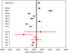 |
Fig. 4. Line-of-sight velocity of GCs, PNe, and NGC 474. The black dashed line shows the line-of-sight velocity of the shell, and the gray shadow its uncertainty. |
The results of the SSP analysis are shown in Fig. 5 and summarized in Table 1. The low S/N of GC 3 and GC 6 (below 10 pix−1) do not allow the fit from pPXF to converge in terms of stellar populations of these GCs and are not shown in that figure. Our estimation gives the shell an intermediate age and metallicity, that is,  Gyr and [M/H] =
  . We note that these ages and metallicities are significantly lower than those of the host galaxy as determined from the SAURON observations: 7.65 ± 1.39 Gyr and [M/H] = −0.12 ± 0.05 within 1 Re (McDermid et al. 2015).
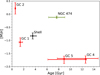 |
Fig. 5. Estimated age and metallicity, assuming an SSP, for the shell and GC 1, GC 2, GC 4, and GC 5. The data points of GC 4 and GC 5 were slightly shifted for visualization purposes. The data point for NGC 474 (mass-weighted age within 1 Re) comes from McDermid et al. (2015). |
Results of the full spectral fitting procedure.
Globular clusters 4 and 5 are estimated to have a low metallicities and advanced ages (above 9 Gyr), which is consistent with their being old GCs. Their masses are estimated to be around 105 M⊙ from the fit. Their metallicities are similar to the so-called blue GCs (Brodie & Strader 2006). GC 1 and GC 2 are estimated to have higher metallicities and much younger ages of around 1 Gyr. The estimated masses for these clusters are, respectively, 2.50 × 10⁴ M⊙ and 5.91 × 10⁴ M⊙.
3.2. Spectral indices
As a complementary method, we estimated age, metallicities, and α-element enrichment from the standardized Lick/IDS system2 (Worthey et al. 1994). We show two diagnostic plots in Fig. 6, making use of the theoretical Lick indices for the MILES spectral library from Thomas et al. (2010). The error bars are the dispersion of the results of the Lick indices measurement on the re-noised spectra used for the measurement of the uncertainties in the previous section. We only show the result for the stellar shell, GC1, and GC2. The other objects have too low S/Ns, and thus a significant fraction of their re-noised spectra have a negative equivalent width for at least one of the absorption lines of interest (more than 25% against maximum one for the shell, GC1, and GC2).
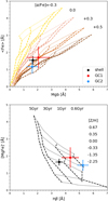 |
Fig. 6. Lick/IDS indices measured from the MUSE spectra of the shell, GC1, and GC2. Definitions of the indices are given in the text. The model grids are from Thomas et al. (2010) with isochrones of 0.6, 1, 3, and 5 Gyr in dashed lines and iso-metallicities of −2.25, −1.35, −0.33, 0.0, 0.35, and 0.67 dex in dotted lines. Upper panel: grids are color-coded with respect to α-enrichment. The isochrones go from the leftmost (0.6 Gyr) to the rightmost one (5 Gyr). Lower panel: grid is shown for [α/Fe] = 0.3. The isochrones go from the rightmost (0.6 Gyr) to the leftmost one (5 Gyr), and iso-metallicities go from the lowest one (−2.32) to the highest one (0.67). |
The first diagnostic uses the Mgb index and ⟨Fe⟩, defined as the average between Fe5270 and Fe5335 (Evstigneeva et al. 2007), which allowed us to probe the α-enrichment of the stellar population. For the ages considered (below 5 Gyr), we see that the spectral indices of these objects are consistent with an α-enrichment [α/Fe] = 0.3, but with rather large error bars due to the low S/N. We note that globular clusters are typically enriched to [α/Fe] = 0.3−0.5 (see review by Brodie & Strader 2006).
The second diagnostic uses the age-sensitive index Hβ and the total metallicity-sensitive index [MgFe]′ =  (Evstigneeva et al. 2007). For GC 2, the two methods give very similar results. However, the Lick indices suggest a younger age and higher metallicities for the shell and GC 1 than our full fitting method. For the shell, Lick Indices suggest [M/H] ∼ −0.33 and an age between 1 and 3 Gyr. For GC 1, they suggest [M/H] ∼ −0.15 and an age around 0.8 Gyr but with large uncertainties. We note that Lick indices do not show a metallicity difference between the two GCs, unlike the full spectral analysis. This second method confirms the trend that GC 1 and GC 2 are younger than the light-averaged stellar population in the stellar shell. We discuss the age difference between the two GCs in Sect. 4.2.
Lastly, the color-color diagram of detected GCs from the L17 catalog is shown in Fig. 7. The estimated young ages of GC 1 and GC 2 are confirmed by their blue color (g − i < 0.5 mag), which excluded them from the L17 analysis. We note that GC 3 has similar (u − g, g − i) colors to GC 1 and GC 2, and it was also rejected as a GC candidate from the L17 analysis. However, its low S/N spectrum does not allow an estimate of its age and metallicity. These three GC candidates have bluer colors than the shell (g − i = 0.6 mag, L17). The origin of these GCs is discussed in the following section.
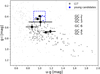 |
Fig. 7. Color-color diagram of point source detections in L17, corrected for foreground dust extinction. The thick points are the GC candidates selected by L17, while the light points were rejected. The six GCs within our field of view are shown as black squares, with their names on the right-hand side. The blue square and points show the selection of the GC candidates considered as young candidates in Sect. 4. |
4. Discussion
4.1. What is the progenitor of the shell?
Numerical simulations have shown that shell formation could emerge from relatively major mergers (> 1:10 in stellar mass ratio; Pop et al. 2018; Karademir et al. 2019). One may wonder if the physical quantities we derived may constrain the mass of the progenitor of the shell. In the following, we assume that the stars in the shell originate from a lower mass companion, the progenitor, and estimate the post-merger mass of NGC 474 to 1010.9 M⊙ (Cappellari et al. 2013).
The estimated metallicity of the stars in the shell is [M/H] =  . Assuming that this value is a good estimation of the mean metallicity of the progenitor, that is, no strong initial metallicity gradients in the progenitor, the empirical stellar mass-metallicity relation gives an estimated mass of
  M⊙ (derived from Eq. (4) of Kirby et al. 2013, accounting for the uncertainties from both their fit and our metallicity measurement). This would imply a merger ratio of 1:109 with 1σ lower and upper limits of, respectively, 1:305 and 1:37.
The stellar mass of a galaxy can also be roughly assessed independently via the number of PNe it hosts and its luminosity. The total number of PNe per bolometric luminosity in the brightest 1 mag of the luminosity distribution is typically α1 = 3 × 10⁻⁷/40 PNe/L⊙ (Buzzoni et al. 2006; the factor 1/40 being derived for the canonical PN luminosity function). We detected six PNe with M5007 between −4.51 and −3.51 mag. Assuming that these six PNe are associated with the stellar population of the shell progenitor and not the halo of NGC 474, which is reasonable given their similar line-of-sight velocity, we can estimate a bolometric luminosity of the shell of Lbol ≃ 8 × 10⁸ L⊙. We note that the PNe systems around some shell galaxy are outliers of typical scaling relations (Buzzoni et al. 2006).
In L17, an absolute magnitude Mg ∼ −17.0 mag and Mi ∼ −17.6 mag for the shell were measured. We assumed a conservative error of 0.3 mag in both bands and used the color-dependant mass-to-light ratio from Roediger & Courteau (2015) with uncertainty 0.29 in solar units. Using M⊙, i = 4.53 mag (Willmer 2018), one obtains an estimation of the stellar mass in the shell of 5.6 × 10⁸ M⊙, with respective 1σ lower and upper limits: 1.7 × 10⁸ M⊙ and 1.9 × 10⁹ M⊙. We note that this estimation falls in the same ballpark as the rough estimate derived from the number of PNe.
Given that NGC 474 is surrounded by many shells and that the shells are expected to host only a fraction of the stellar light from the progenitor (around 25 to 30% from simulations, see Hernquist & Spergel 1992; Ebrová et al. 2020), the progenitor should be more massive than the above estimation, which considered only the stellar shell. This also holds for the PNe estimation, assuming they follow the spatial distribution of the progenitor stars. Assuming that the shell studied here hosts 50 ± 10% of the stars in the outer shell system created by the interaction (see Fig. 1), and assuming that the shells host 30 ± 10% of the progenitor stellar mass, the luminosity gives an estimated progenitor mass of  M⊙. This translates into a merger ratio of 1:21, with respective lower and upper σ limits of 1:72 and 1:6.
The estimations from the stellar metallicity and the luminosity, summarized in Table 2, differ by a factor of five, but given the large error bars, the two values are inconsistent by only ∼1σ. Nevertheless, one should note that we have so far assumed that the progenitor has a constant metallicity, which is a disputable hypothesis.
Progenitor mass and merger ratio estimates derived from a given constraint.
Resolved metallicity gradients in local star-forming galaxies from the CALIFA survey show that a stellar metallicity as low as [M/H] = −0.83 is attained beyond 2.5 effective radius in galaxies with stellar mass above 109.1 M⊙ only for rare outliers, the constraint being stricter in groups (González Delgado et al. 2015; Coenda et al. 2020). However, one should note that other surveys, such as MaNGA, did find steeper metallicity gradients in their local star-forming galaxy samples, with metallicities as low as [M/H] = −0.7 at a 1.5 effective radius, even for 1010.5 − 11 M⊙ galaxies (Lian et al. 2018).
On one hand, the observed stellar shell may have formed via a ∼1 : 100 merger event, and in this case the observed shell would contain most of the stars of the progenitor, contrarily to the 15% assumed here. The various outer shells would then come from different progenitors, possibly including the primary galaxy. On the other hand, the observed stellar shell may have formed via a ∼1 : 20 merger event, from a galaxy with a stellar mass of a few 109 M⊙ and lower mean metallicity than typical galaxies of similar stellar mass, or with a metallicity gradient.
These two scenarios might be further explored using spectroscopic data of the other shells and a chemo-dynamical numerical model of the collision. We further note that Alabi et al. (2020)3 suggested a more massive progenitor, namely ≃1010 M⊙, based on a higher metallicity measurement. One would thus need observations revealing the kinematics and the stellar populations – age and metallicity – within the other shells, for instance using integral field spectroscopy. Given the low surface brightness of the shells and the long exposure time on an 8-meter class telescope used for this study, we estimate that such a study will only be made possible by the upcoming generation of 30-meter class optical telescopes. Once these measures are obtained, numerical simulations using different progenitor masses and metallicity gradients would be needed to show which of the proposed configurations are actually achievable within the observation constraints.
4.2. Could the shell-forming event trigger massive star-cluster formation?
From cosmological zoom simulations, Mancillas et al. (2019a) estimated that stellar shells can remain visible for 3 to 4 Gyr. In Sect. 3, we estimated that GC 1 and GC 2 are younger than 1.5 Gyr. One may thus wonder if they were formed during the event that formed the stellar shell.
Observations and simulations of interactions of galaxies have shown that such events could trigger the formation of star clusters, similar in mass to GC 1 and GC 2 (see e.g., Whitmore et al. 2010; Renaud et al. 2015; Lahén et al. 2019). Sikkema et al. (2006) found hints for newly formed GCs in the nucleus of two shell galaxies (Type II NGC 2865 and Type III NGC 7626), but not for NGC 474. We noted in Sect. 3 that GC 1 and GC 2 have different ages and metallicities. To explain that, one may estimate the free-fall time at the radius of the shell, which is 30 kpc. Via abundance matching (Behroozi et al. 2013; Diemer & Kravtsov 2015), one may estimate that the most likely halo to host NGC 474 would have a total mass of 9 × 10¹¹ M⊙ and a virial radius of 1200 kpc, which gives a free-fall time of about 100 Myr. This means that the GCs have already passed close to the nucleus of NGC 474 several times since their formation, and it is possible that their formation happened at different passages of the associated material close to that nucleus.
One way to test the hypothesis of triggered star-cluster formation is to check whether we see traces of star formation from the same epoch in the nucleus of NGC 474, where we may expect the build-up of a gas reservoir leading to a potential starburst. We note that Jeong et al. (2012) and Zaritsky et al. (2014) classified NGC 474 as a “blue outlier” among early-type and lenticular galaxies because of its relatively blue color and elevated near-UV emission. Moreover, Sikkema et al. (2007) noticed pronounced dust lanes (estimated mass of ∼104 M⊙) in the central 15″ of NGC 474, which align with the location of ionized gas. No molecular gas was found in the central region of NGC 474 (upper limit: M(H2) < 107.7 M⊙, see Combes et al. 2007; Mancillas et al. 2019b). Schiminovich et al. (1997) and Rampazzo et al. (2006) found a HI tail due to the interaction with NGC 470 (the spiral galaxy westward of NGC 474 in Fig. 1), but it is not superimposed with the shell.
To investigate the presence of a young stellar population in the host galaxy, we used the central kpc of the SAURON data cube centered on NGC 474 from Cappellari et al. (2011) and the pPXF regularization procedure from Cappellari (2017), with three-degree multiplicative Legendre polynomials and the previous eMILES library. To avoid degeneracies due to the presence of emission lines, namely Hβ and the [OIII] doublet, we performed a first fit by masking the location of these lines, and we fixed the obtained velocity and velocity dispersion for a second fit enabling emission lines. Uncertainties on the fit were obtained with the bootstrap method used for the MUSE data.
The regularized fit to the data and the weights of the different templates are shown, respectively, in the upper and lower panels of Fig. 8. We stress that the full SSP library is considered by pPXF, but only some of them obtain a nonzero weight from the regularization procedure. On top of old and metal-rich templates, typical of elliptical galaxies, the regularization gives a non-zero weight to templates of age and metallicity similar to GC 1 and GC 2 (see Fig. 5). The regularization also gave nonzero weights to very metal-poor templates, at the limit of our metallicity grid. To estimate the significance of these metal-poor templates on our estimation, we created two templates: “old, high Z” and “old + young, high Z”, which, respectively, contains the old and metal-rich (age > 7 Gyr and [M/H] > −2), and all the metal-rich ([M/H] > −2) templates used in the regularized fit with their respective weights. Then we fit the SAURON spectrum with each of these templates, following the same procedure as above. The results are shown in Fig. 9. We see that the “old, high-Z” population alone struggles particularly to account for the region around the Hβ and Mgb absorption lines. Adding the young and metal-rich population improves the fit significantly, especially around the Hβ line. Adding this population reduces the χ2 by a factor 2.4. Adding the metal-poor population improves the fit around the Fe lines (observed wavelength ∼5054 Å for line-of-sight velocity of 2315 km s−1) while overestimating the flux in the Mgb line. Adding this population reduces the χ2 by 10%.
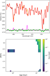 |
Fig. 8. Upper panel: best fit for the SAURON data of NGC 474 (central kpc), from the pPXF procedure. The data is in black, the fit in red for the star component, and yellow for the gas component. The green points show the residuals and the pink line highlights the ionized gas component fit: from left to right, Hβ and the [OIII] doublet. Lower panel: weights of the different templates used by the regularized fit. Only colored regions are contained in the resulting fit. See text for details. |
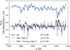 |
Fig. 9. Best fits, residuals, and χ2 values corresponding to the procedure described in the text. The residuals have been multiplied by 10 and shifted by a constant 0.5 offset for the sake of visualization. The flux unit is arbitrary. |
The fit infers a total mass for the young and metal-rich component of 3.22 ± 1.37 × 10⁷ M⊙, to be compared with 4.00 ± 0.83 × 10⁹ M⊙ for the old and metal-rich component. The young (old) and metal-poor component in the fit is evaluated as 3% (2.4%) of the young (old) and metal-rich in terms of mass: 1.07 × 10⁶ M⊙ (9.52 × 10⁷ M⊙).
Given the low level of improvement of the fit by adding these very metal-poor populations and their low relative mass contributions, we discard them in the following. The inclusion of these populations at the limit of our metallicity grid and for the same ages as the most important contributors to the fit might be due to the imperfection of the used SSP models, in particular in terms of [α/Fe] (we only used “base models”, see discussion in Vazdekis et al. 2016).
The SAURON spectrum of NGC 474 therefore supports the hypothesis of a nuclear starburst around 1 Gyr ago. We note that this timescale is similar to the estimated ages of the massive stellar clusters, and it suggests that both the starburst and cluster formation could have been caused by a single galaxy merger. However, we warn that the structure of NGC 474 is complex (see e.g., Sikkema et al. 2007) and that this young stellar component cannot yet be unambiguously connected to the shell.
One may thus wonder what the origin of the gas that fueled this starburst and the formation of the GCs is. Indeed, the nucleus of NGC 474 does not host any detectable H2, and we note that no HI has been detected at the vicinity of the shell (Schiminovich et al. 1997; Rampazzo et al. 2006; Mancillas et al. 2019b). This suggests that these episodes of star formation were very efficient at consuming or ejecting the gas and calls for a dedicated numerical study of star cluster formation in shell-forming galaxy interactions.
Lastly, we located all the GC candidates around NGC 474 (see field of view in Fig. 10) with similar colors to the confirmed young GC 1 and 2. We chose GC candidates with 0.3 < g − i < 0.5 and 0.9 < u − g < 1.1, depicted as “young candidates” in Fig. 7. There are nine young candidates in total, including GCs 1, 2, and 3. There is one more young candidate in the MUSE field-of-view. After verification, this source was discarded from the present analysis because of its very low S/N = 2.8 pix−1, which did not permit any reliable analysis. Apart from GC 1 and GC 2 (with, respectively, mg = 23.04 ± 0.02 mag and 22.19 ± 0.01 mag), these candidates have mg between 24 and 25 mag. We note that their relative faintness would not allow age and metallicity measurements using MUSE with less than 10.2 h of on-source integration. These six young candidates are shown by cyan circles in Fig. 10. We note that they are located in the vicinity of the studied shell, inner stellar shells, or tidal features, suggesting a possible link with the events that created these structures.
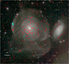 |
Fig. 10. True-color image from Megacam at CFHT with locations of the GC candidates around NGC 474. Young candidates are shown in cyan, old candidates in red. The GC candidates for which we have MUSE spectroscopy are shown with squares. The white line spans 1 arcmin. |
5. Conclusion
We used MUSE at VLT to study the origin of an external stellar shell around the host galaxy NGC 474. We find eight PNe and six GC candidates (including three candidates from Lim et al. 2017) that are kinematically associated with the stellar shell. Stars from the shell have a luminosity-weighted age below that of the host:  Gyr. We show that the shell has an intermediate metallicity, [M/H] =
  , and a possible α-enrichment, [α/Fe] ∼ 0.3.
Assuming the material of the shell comes from a lower mass companion, and that the latter had no initial metallicity gradient, the measured stellar metallicity would constrain the mass of the progenitor to be around 7.4 × 10⁸ M⊙, implying a merger mass ratio of about 1:100. However, our census of PNe and archival photometry of the shell would suggest a higher merger ratio, namely 1:20. While this discrepancy is only significant at the 1σ level, different scenarios are discussed, namely that the shell contains a high proportion of the stars from the progenitor, that the progenitor has a lower stellar metallicity than is typical for a given stellar mass, or that the stars of the shell originate fromthe low-metallicity outskirts of a more massive galaxy with a metallicity gradient. Each of these scenarios could be assessed with dedicated chemo-dynamical observations and numerical simulations.
Full spectral fitting of the four GC candidates with high enough S/N shows that two of them are consistent with being old globular clusters while the other two show signs of young ages (< 1.5 Gyr) and relatively high metallicity ([M/H] > −1.1). The study of the Lick indices confirms the trend that GC 1 and GC 2 are younger than the stars in the shell. Their different ages and metallicities hint to a formation at a different passage of the associated material close to the nucleus. This is consistent with their blue color, which excluded them from previous analyses of GCs in this system. The regularization of full spectral fitting on SAURON data of the central kpc of NGC 474 suggests the presence of a relatively young stellar population, with an age and metallicity similar to those of these young GC candidates. This suggests that these young GC candidates might have formed during the merging event that caused the formation of the stellar shell. We note the presence of nine GC candidates with similar colors around NGC 474, all fainter than GC 2, which is the brightest young cluster candidate with an estimated mass of ∼6 × 10⁴ M⊙.
This data thus supports the scenario in which these stellar shells formed from a progenitor with low overall metallicity, or from its low-metallicity outskirts, and during a merger that might have possibly triggered the formation of massive star clusters and/or triggered a nuclear starburst in the host. This calls for dedicated numerical studies to confirm or disprove such a scenario.
Available here: http://www-astro.physics.ox.ac.uk/atlas3d/. See SAURON data from Paper I: (Cappellari et al. 2011).
We used the pyphot package available at this address: https://mfouesneau.github.io/docs/pyphot/index.html
This article was made public during the refereeing process of the present article.
Acknowledgments
We thank the referee for insightful comments that help improve this paper. JF would like to thank the ESO User Support Department for their great help on performing these observations. The authors thank Richard McDermid and Harald Kuntschner for interesting discussions respectively about NGC 474 and Lick Indices. C.L. acknowledges support from the National Natural Science Foundation of China (NSFC, Grant No. 11673017, 11833005, 11933003, 11621303, 11973033 and 11203017).
References
- Alabi, A. B., Ferré-Mateu, A., Forbes, D. A., Romanowsky, A. J., & Brodie, J. P. 2020, MNRAS, 497, 626 [CrossRef] [Google Scholar]
- Amorisco, N. C. 2015, MNRAS, 450, 575 [NASA ADS] [CrossRef] [Google Scholar]
- Arp, H. 1966, ApJS, 14, 1 [NASA ADS] [CrossRef] [Google Scholar]
- Atkinson, A. M., Abraham, R. G., & Ferguson, A. M. N. 2013, ApJ, 765, 28 [NASA ADS] [CrossRef] [Google Scholar]
- Behroozi, P. S., Wechsler, R. H., & Conroy, C. 2013, ApJ, 770, 57 [NASA ADS] [CrossRef] [Google Scholar]
- Bertin, E., & Arnouts, S. 1996, A&AS, 117, 393 [NASA ADS] [CrossRef] [EDP Sciences] [Google Scholar]
- Bílek, M., Jungwiert, B., Jílková, L., et al. 2013, A&A, 559, A110 [NASA ADS] [CrossRef] [EDP Sciences] [Google Scholar]
- Bílek, M., Cuillandre, J. C., Gwyn, S., et al. 2016, A&A, 588, A77 [NASA ADS] [CrossRef] [EDP Sciences] [Google Scholar]
- Blom, C., Forbes, D. A., Foster, C., Romanowsky, A. J., & Brodie, J. P. 2014, MNRAS, 439, 2420 [NASA ADS] [CrossRef] [Google Scholar]
- Brodie, J. P., & Strader, J. 2006, ARA&A, 44, 193 [NASA ADS] [CrossRef] [Google Scholar]
- Buzzoni, A., Arnaboldi, M., & Corradi, R. L. M. 2006, MNRAS, 368, 877 [NASA ADS] [CrossRef] [Google Scholar]
- Cappellari, M. 2017, MNRAS, 466, 798 [NASA ADS] [CrossRef] [Google Scholar]
- Cappellari, M., Emsellem, E., Krajnović, D., et al. 2011, MNRAS, 416, 1680 [NASA ADS] [CrossRef] [Google Scholar]
- Cappellari, M., McDermid, R. M., Alatalo, K., et al. 2013, MNRAS, 432, 1862 [NASA ADS] [CrossRef] [Google Scholar]
- Charmandaris, V., Combes, F., & van der Hulst, J. M. 2000, A&A, 356, L1 [NASA ADS] [Google Scholar]
- Coenda, V., Mast, D., Muriel, H., & Martínez, H. J. 2020, A&A, 642, A132 [CrossRef] [EDP Sciences] [Google Scholar]
- Combes, F., Young, L. M., & Bureau, M. 2007, MNRAS, 377, 1795 [NASA ADS] [CrossRef] [Google Scholar]
- de Zeeuw, P. T., Bureau, M., Emsellem, E., et al. 2002, MNRAS, 329, 513 [NASA ADS] [CrossRef] [Google Scholar]
- Diemer, B., & Kravtsov, A. V. 2015, ApJ, 799, 108 [NASA ADS] [CrossRef] [Google Scholar]
- Duc, P. A., Brinks, E., Springel, V., et al. 2000, AJ, 120, 1238 [NASA ADS] [CrossRef] [Google Scholar]
- Duc, P.-A., Cuillandre, J.-C., Karabal, E., et al. 2015, MNRAS, 446, 120 [NASA ADS] [CrossRef] [Google Scholar]
- Durrell, P. R., Mihos, J. C., Feldmeier, J. J., Jacoby, G. H., & Ciardullo, R. 2003, ApJ, 582, 170 [NASA ADS] [CrossRef] [Google Scholar]
- Ebrová, I., Jílková, L., Jungwiert, B., et al. 2012, A&A, 545, A33 [NASA ADS] [CrossRef] [EDP Sciences] [Google Scholar]
- Ebrová, I., Bílek, M., Yıldız, M. K., & Eliášek, J. 2020, A&A, 634, A73 [CrossRef] [EDP Sciences] [Google Scholar]
- Emsellem, E., Cappellari, M., Peletier, R. F., et al. 2004, MNRAS, 352, 721 [NASA ADS] [CrossRef] [Google Scholar]
- Emsellem, E., van der Burg, R. F. J., Fensch, J., et al. 2019, A&A, 625, A76 [NASA ADS] [CrossRef] [EDP Sciences] [Google Scholar]
- Evstigneeva, E. A., Gregg, M. D., Drinkwater, M. J., & Hilker, M. 2007, AJ, 133, 1722 [NASA ADS] [CrossRef] [Google Scholar]
- Fensch, J., van der Burg, R. F. J., Jeřábková, T., et al. 2019, A&A, 625, A77 [NASA ADS] [CrossRef] [EDP Sciences] [Google Scholar]
- Forbes, D. A., Cortesi, A., Pota, V., et al. 2012, MNRAS, 426, 975 [NASA ADS] [CrossRef] [Google Scholar]
- Foster, C., Lux, H., Romanowsky, A. J., et al. 2014, MNRAS, 442, 3544 [CrossRef] [Google Scholar]
- González Delgado, R. M., García-Benito, R., Pérez, E., et al. 2015, A&A, 581, A103 [NASA ADS] [CrossRef] [EDP Sciences] [Google Scholar]
- Hau, G. K. T., Balcells, M., & Carter, D. 1996, in New Light on Galaxy Evolution, eds. R. Bender, & R. L. Davies, IAU Symp., 171, 388 [CrossRef] [Google Scholar]
- Hendel, D., & Johnston, K. V. 2015, MNRAS, 454, 2472 [NASA ADS] [CrossRef] [Google Scholar]
- Hernquist, L., & Spergel, D. N. 1992, ApJ, 399, L117 [NASA ADS] [CrossRef] [Google Scholar]
- Jeong, H., Yi, S. K., Bureau, M., et al. 2012, MNRAS, 423, 1921 [NASA ADS] [CrossRef] [Google Scholar]
- Johnston, K. V., Bullock, J. S., Sharma, S., et al. 2008, ApJ, 689, 936 [NASA ADS] [CrossRef] [Google Scholar]
- Karademir, G. S., Remus, R.-S., Burkert, A., et al. 2019, MNRAS, 487, 318 [NASA ADS] [CrossRef] [Google Scholar]
- Kirby, E. N., Cohen, J. G., Guhathakurta, P., et al. 2013, ApJ, 779, 102 [NASA ADS] [CrossRef] [Google Scholar]
- Krajnović, D., Emsellem, E., Cappellari, M., et al. 2011, MNRAS, 414, 2923 [NASA ADS] [CrossRef] [Google Scholar]
- Kuntschner, H., Emsellem, E., Bacon, R., et al. 2010, MNRAS, 408, 97 [NASA ADS] [CrossRef] [Google Scholar]
- Lahén, N., Naab, T., Johansson, P. H., et al. 2019, ApJ, 879, L18 [NASA ADS] [CrossRef] [Google Scholar]
- Lian, J., Thomas, D., Maraston, C., et al. 2018, MNRAS, 476, 3883 [NASA ADS] [CrossRef] [Google Scholar]
- Lim, S., Peng, E. W., Duc, P.-A., et al. 2017, ApJ, 835, 123 [NASA ADS] [CrossRef] [Google Scholar]
- Longobardi, A., Arnaboldi, M., Gerhard, O., & Mihos, J. C. 2015, A&A, 579, L3 [NASA ADS] [CrossRef] [EDP Sciences] [Google Scholar]
- Mancillas, B., Duc, P.-A., Combes, F., et al. 2019a, A&A, 632, A122 [NASA ADS] [CrossRef] [EDP Sciences] [Google Scholar]
- Mancillas, B., Combes, F., & Duc, P.-A. 2019b, A&A, 630, A112 [NASA ADS] [CrossRef] [EDP Sciences] [Google Scholar]
- Martínez-Delgado, D., Gabany, R. J., Crawford, K., et al. 2010, AJ, 140, 962 [NASA ADS] [CrossRef] [Google Scholar]
- McDermid, R. M., Alatalo, K., Blitz, L., et al. 2015, MNRAS, 448, 3484 [NASA ADS] [CrossRef] [Google Scholar]
- Mihos, J. C., Harding, P., Feldmeier, J., & Morrison, H. 2005, ApJ, 631, L41 [NASA ADS] [CrossRef] [Google Scholar]
- Mullan, B., Konstantopoulos, I. S., Kepley, A. A., et al. 2011, ApJ, 731, 93 [NASA ADS] [CrossRef] [Google Scholar]
- Müller, O., Rich, R. M., Román, J., et al. 2019, A&A, 624, L6 [NASA ADS] [CrossRef] [EDP Sciences] [Google Scholar]
- Pence, W. D. 1986, ApJ, 310, 597 [NASA ADS] [CrossRef] [Google Scholar]
- Pop, A.-R., Pillepich, A., Amorisco, N. C., & Hernquist, L. 2018, MNRAS, 480, 1715 [NASA ADS] [CrossRef] [Google Scholar]
- Prieur, J. L. 1990, in Status of Shell Galaxies, ed. R. Wielen, 72 [Google Scholar]
- Quinn, P. J. 1984, ApJ, 279, 596 [NASA ADS] [CrossRef] [Google Scholar]
- Rampazzo, R., Alexander, P., Carignan, C., et al. 2006, MNRAS, 368, 851 [NASA ADS] [CrossRef] [Google Scholar]
- Renaud, F., Bournaud, F., & Duc, P.-A. 2015, MNRAS, 446, 2038 [NASA ADS] [CrossRef] [Google Scholar]
- Roediger, J. C., & Courteau, S. 2015, MNRAS, 452, 3209 [NASA ADS] [CrossRef] [Google Scholar]
- Schiminovich, D., van Gorkom, J., van der Hulst, T., Oosterloo, T., & Wilkinson, A. 1997, in The Nature of Elliptical Galaxies; 2nd Stromlo Symposium, eds. M. Arnaboldi, G. S. Da Costa, & P. Saha, ASP Conf. Ser., 116, 362 [Google Scholar]
- Sikkema, G., Peletier, R. F., Carter, D., Valentijn, E. A., & Balcells, M. 2006, A&A, 458, 53 [NASA ADS] [CrossRef] [EDP Sciences] [Google Scholar]
- Sikkema, G., Carter, D., Peletier, R. F., et al. 2007, A&A, 467, 1011 [NASA ADS] [CrossRef] [EDP Sciences] [Google Scholar]
- Soto, K. T., Lilly, S. J., Bacon, R., Richard, J., & Conseil, S. 2016, MNRAS, 458, 3210 [NASA ADS] [CrossRef] [Google Scholar]
- Tal, T., van Dokkum, P. G., Nelan, J., & Bezanson, R. 2009, AJ, 138, 1417 [NASA ADS] [CrossRef] [Google Scholar]
- Thomas, D., Maraston, C., Schawinski, K., Sarzi, M., & Silk, J. 2010, MNRAS, 404, 1775 [NASA ADS] [Google Scholar]
- Turnbull, A. J., Bridges, T. J., & Carter, D. 1999, MNRAS, 307, 967 [NASA ADS] [CrossRef] [Google Scholar]
- van Dokkum, P. G., Abraham, R., & Merritt, A. 2014, ApJ, 782, L24 [NASA ADS] [CrossRef] [Google Scholar]
- Vazdekis, A., Koleva, M., Ricciardelli, E., Röck, B., & Falcón-Barroso, J. 2016, MNRAS, 463, 3409 [Google Scholar]
- Weilbacher, P. M., Palsa, R., Streicher, O., et al. 2020, A&A, 641, A28 [CrossRef] [EDP Sciences] [Google Scholar]
- White, S. D. M., & Rees, M. J. 1978, MNRAS, 183, 341 [NASA ADS] [CrossRef] [Google Scholar]
- Whitmore, B. C., Chandar, R., Schweizer, F., et al. 2010, AJ, 140, 75 [NASA ADS] [CrossRef] [Google Scholar]
- Wilkinson, A., Sparks, W. B., Carter, D., & Malin, D. A. 1987, in Structure and Dynamics of Elliptical Galaxies, ed. P. T. de Zeeuw, IAU Symp., 127, 465 [NASA ADS] [CrossRef] [Google Scholar]
- Williams, B. A., Yun, M. S., & Verdes-Montenegro, L. 2002, AJ, 123, 2417 [NASA ADS] [CrossRef] [Google Scholar]
- Willmer, C. N. A. 2018, ApJS, 236, 47 [NASA ADS] [CrossRef] [Google Scholar]
- Worthey, G., Faber, S. M., Gonzalez, J. J., & Burstein, D. 1994, ApJS, 94, 687 [NASA ADS] [CrossRef] [Google Scholar]
- Yun, M. S., Ho, P. T. P., & Lo, K. Y. 1994, Nature, 372, 530 [NASA ADS] [CrossRef] [PubMed] [Google Scholar]
- Zaritsky, D., Gil de Paz, A., & Bouquin, A. R. Y. K. 2014, ApJ, 780, L1 [NASA ADS] [CrossRef] [Google Scholar]
Appendix A: GC spectra and fits
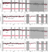 |
Fig. A.1. continued. |
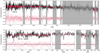 |
Fig. A.1. continued. |
All Tables
All Figures
|
Fig. 1. Left: true color image constructed from the MUSE data using the g, r, and i filters of Megacam at CFHT as colors. The locations of the detected PNe are shown with blue circles. In green, we show the detected GCs. GCs 4, 5, and 6 were part of the L17 sample: their number in that catalog is given after their name. The two red circles show detections that were classified by L17 as GC candidates but are not confirmed with the present data. Right: zoom-out true-color image from CFHT (g, r, i bands from Duc et al. 2015). The MUSE and SKY pointings are shown, respectively, in white and yellow. The SAURON pointing from de Zeeuw et al. (2002) is shown in blue. The MUSE and SAURON pointings are, respectively, 1′×1′ and 33″ × 41″ wide. Assuming a distance to NGC 474 of 30.9 Mpc (Cappellari et al. 2011), 1′ encompasses around 8.9 kpc. North is up and west is right. |
| In the text | |
|
Fig. 2. Comparison between spectrum and best SSP fit from pPXF for the shell and GC 2. The three plots in the bottom part of each panel show zooms of the important absorption lines. The gray regions are not taken into account for the fit. The scatter points show the residuals. |
| In the text | |
|
Fig. 3. Spectra of the eight PNe candidates. The location of the [OIII] doublet at the redshift of NGC 474 is shown with gray dashed lines. |
| In the text | |
|
Fig. 4. Line-of-sight velocity of GCs, PNe, and NGC 474. The black dashed line shows the line-of-sight velocity of the shell, and the gray shadow its uncertainty. |
| In the text | |
|
Fig. 5. Estimated age and metallicity, assuming an SSP, for the shell and GC 1, GC 2, GC 4, and GC 5. The data points of GC 4 and GC 5 were slightly shifted for visualization purposes. The data point for NGC 474 (mass-weighted age within 1 Re) comes from McDermid et al. (2015). |
| In the text | |
|
Fig. 6. Lick/IDS indices measured from the MUSE spectra of the shell, GC1, and GC2. Definitions of the indices are given in the text. The model grids are from Thomas et al. (2010) with isochrones of 0.6, 1, 3, and 5 Gyr in dashed lines and iso-metallicities of −2.25, −1.35, −0.33, 0.0, 0.35, and 0.67 dex in dotted lines. Upper panel: grids are color-coded with respect to α-enrichment. The isochrones go from the leftmost (0.6 Gyr) to the rightmost one (5 Gyr). Lower panel: grid is shown for [α/Fe] = 0.3. The isochrones go from the rightmost (0.6 Gyr) to the leftmost one (5 Gyr), and iso-metallicities go from the lowest one (−2.32) to the highest one (0.67). |
| In the text | |
|
Fig. 7. Color-color diagram of point source detections in L17, corrected for foreground dust extinction. The thick points are the GC candidates selected by L17, while the light points were rejected. The six GCs within our field of view are shown as black squares, with their names on the right-hand side. The blue square and points show the selection of the GC candidates considered as young candidates in Sect. 4. |
| In the text | |
|
Fig. 8. Upper panel: best fit for the SAURON data of NGC 474 (central kpc), from the pPXF procedure. The data is in black, the fit in red for the star component, and yellow for the gas component. The green points show the residuals and the pink line highlights the ionized gas component fit: from left to right, Hβ and the [OIII] doublet. Lower panel: weights of the different templates used by the regularized fit. Only colored regions are contained in the resulting fit. See text for details. |
| In the text | |
|
Fig. 9. Best fits, residuals, and χ2 values corresponding to the procedure described in the text. The residuals have been multiplied by 10 and shifted by a constant 0.5 offset for the sake of visualization. The flux unit is arbitrary. |
| In the text | |
|
Fig. 10. True-color image from Megacam at CFHT with locations of the GC candidates around NGC 474. Young candidates are shown in cyan, old candidates in red. The GC candidates for which we have MUSE spectroscopy are shown with squares. The white line spans 1 arcmin. |
| In the text | |
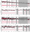 |
Fig. A.1. Same as Fig. 2. |
| In the text | |
|
Fig. A.1. continued. |
| In the text | |
|
Fig. A.1. continued. |
| In the text | |
Current usage metrics show cumulative count of Article Views (full-text article views including HTML views, PDF and ePub downloads, according to the available data) and Abstracts Views on Vision4Press platform.
Data correspond to usage on the plateform after 2015. The current usage metrics is available 48-96 hours after online publication and is updated daily on week days.
Initial download of the metrics may take a while.