| Issue |
A&A
Volume 644, December 2020
|
|
|---|---|---|
| Article Number | A140 | |
| Number of page(s) | 11 | |
| Section | Galactic structure, stellar clusters and populations | |
| DOI | https://doi.org/10.1051/0004-6361/202038346 | |
| Published online | 10 December 2020 | |
Mapping the stellar age of the Milky Way bulge with the VVV
III. High-resolution reddening map⋆,⋆⋆,⋆⋆⋆
1
Instituto de Astrofísica de Canarias, 38205 La Laguna, Tenerife, Spain
e-mail: frsurot@uc.cl
2
Departamento de Astrofísica, Universidad de La Laguna, 38205 La Laguna Tenerife, Spain
3
European Southern Observatory, Karl Schwarzschild-Straße 2, 85748 Garching bei München, Germany
4
Excellence Cluster ORIGINS, Boltzmann-Straße 2, 85748 Garching bei München, Germany
5
UK Astronomy Technology Centre, Royal Observatory, Blackford Hill, Edinburgh EH9 3HJ, UK
6
Instituto de Astrofísica, Pontificia Universidad Católica de Chile, Av. Vicuña Mackenna 4860, Santiago, Chile
7
Millennium Institute of Astrophysics, Av. Vicuña Mackenna 4860, 782-0436 Macul, Santiago, Chile
8
Departamento de Ciencias Físicas, Universidad Andrés Bello, República 220, Santiago, Chile
9
Vatican Observatory, V00120 Vatican City State, Italy
Received:
5
May
2020
Accepted:
21
September
2020
Context. A detailed study of the Galactic bulge stellar population necessarily requires an accurate representation of the interstellar extinction, particularly toward the Galactic plane and center, where severe and differential reddening is expected to vary on sub-arcmin scales. Although recent infrared surveys have addressed this problem by providing extinction maps across the whole Galactic bulge area, dereddened color-magnitude diagrams near the plane and center appear systematically undercorrected, prompting the need for higher resolution. These undercorrections affect any stellar study sensitive to color (e.g., star formation history analyses via color-magnitude diagram fitting), either making them inaccurate or limiting them to small and relatively stable extinction windows where this value is low and better constrained.
Aims. This study is aimed at providing a high-resolution (2 arcmin to ∼10 arcsec) color excess map for the VVV bulge area in J − Ks color.
Methods. We used the MW-BULGE-PSFPHOT catalogs, sampling ∼300 deg2 across the Galactic bulge (|l| < 10° and −10° < b < 5°) to isolate a sample of red clump and red giant branch stars, for which we calculated the average J − Ks color in a fine spatial grid in (l, b) space.
Results. We obtained an E(J − Ks) map spanning the VVV bulge area of roughly 300 deg2, with the equivalent of a resolution between ∼1 arcmin for bulge outskirts (l < 6°) to below 20 arcsec within the central |l| < 1°, and below 10 arcsec for the innermost area (|l| < 1° and |b| < 3°).
Key words: Galaxy: structure / Galaxy: bulge
The map is only available at the CDS via anonymous ftp to cdsarc.u-strasbg.fr (130.79.128.5) or via http://cdsarc.u-strasbg.fr/viz-bin/cat/J/A+A/644/A140
Based on observations taken within the ESO VISTA Public Survey VVV, Program ID 179.B-2002 (PI: Minniti, Lucas).
The result is publicly available at http://basti-iac.oa-teramo.inaf.it/vvvexmap/
© ESO 2020
1. Introduction
Despite the extensive efforts undertaken in the last decade to construct reddening maps in the Galactic bulge, interstellar extinction continues to be one of the most uncertain parameters when studying the stellar populations of the inner regions of the Milky Way. A combination of systematics in the construction of reddening and extinction maps as well as the uncertainties in the extinction law used to obtain reddening-free magnitudes can substantially affect the results, based on both photometric and spectroscopic observations of the central regions of the Galaxy.
The extinction law has been shown to be non-standard and variable in the regions closer to the Galactic plane (see Nataf et al. 2016, for a detailed review), thus results can differ depending on the bands used for each study and the adopted extinction law. On the other hand, the main limitation for the applicability of reddening maps in studies of the Galactic bulge comes from their spatial resolution. Reddening variations on very small scales, down to a few arcseconds, can be seen in maps of specific windows (see for example Gosling et al. 2009). The residual differential reddening within the resolution element of a reddening map can strongly affect the extinction correction of stellar populations or the characterization of the extinction law. As a result, and with the increasing number of photometric and spectroscopic surveys covering the bulge, special attention has been given to improve the spatial scales in which reddening is calculated without compromise from sensitivity. However, wide-field reddening and extinction maps of the Galactic bulge in sub-arcmin scales are not yet available.
With the advent of infrared (IR) and near-IR photometry, the studies of the Galactic bulge have seen advances over the past decade. Large surveys (DENIS – Epchtein 1998; 2MASS – Skrutskie et al. 2006; UKIDSS – Lawrence et al. 2007; VVV(X) – Minniti 2016; GLIMPSE – Benjamin et al. 2003) provided the framework necessary for taking extinction studies to regions of higher extinction, thus, closer to the Galactic plane at considerably higher spatial resolution than previously available. For example, Schultheis et al. (1999) used DENIS photometry to produce color-magnitude diagrams (CMDs) in 2 arcmin windows and compare the location of M giants with theoretical isochrones of stellar populations in the red giant branch (RGB) and asymptotic giant branch (AGB). This comparison was used in Schultheis et al. (1999) to estimate reddening in each of these windows to produce the first high-resolution extinction map of the Galactic plane, including regions with extinctions as large as 35 magnitudes in the optical. However, this study is limited by the sensitivity of DENIS in these regions, in particular, the J-band. Dutra et al. (2003) later produced a map applying the same technique to 2MASS data, but covering a considerably larger area. In this latter case, the limitation for the map comes from the spatial resolution of 2MASS, which is not sufficient to avoid the crowding effects in the high-density, innermost regions of the Galaxy.
This situation improved dramatically thanks to the spatial resolution and depth of near-IR of the VISTA Variables in the Vía Láctea (VVV) survey (Minniti et al. 2010) which allowed different teams to map red-clump (RC) stars (as previously done with optical photometry in the outer bulge) all the way down to the Galactic plane. The first VVV extinction map was presented by Gonzalez et al. (2012) with a spatial resolution ranging from 6 arcmin in the outer bulge to 2 arcmin near the Galactic plane. Extinction maps with the same spatial resolution were constructed using GLIMPSE by Schultheis et al. (2009), following the same isochrone-fitting technique from Schultheis et al. (1999). Since, in the case of the VVV extinction maps, the spatial resolution of the maps was determined by the number of RC stars in the resolution element, the achieved resolution was recently improved to a 1 arcmin resolution thanks to the construction of point spread function (PSF) catalogs (Alonso-García et al. 2018) with deeper and more complete photometry down to the RC magnitude level across the entire bulge region (Gonzalez et al. 2018), achieving the highest coverage/resolution ratio for a 2D extinction map of the Galactic bulge region thus far.
Extinction maps are also useful for identifying windows of low extinction at low latitudes within the plane, which are strategic tools necessary for seeing deeply across the Milky Way. A classic example would be Baade’s Window, which has traditionally been important for studies of the stellar populations in the Galactic bulge. More recently, the VVV survey has allowed for the identification of a couple more windows with relatively low and uniform extinction in the Galactic plane (Minniti et al. 2018; Saito et al. 2020). These windows are: VVV WIN 1713-3939, located at Galactic coordinates (l, b) = (347.4° , − 0.4° ) and with a mean total near-IR extinction of AKs = 0.46 mag; and VVV WIN 1733-3349, located at (l, b) = (−5.2° , − 0.3° ) and with a mean extinction of AKs = 0.61 mag.
However, despite the progress made in this regard, the Galactic center and plane remain a challenge with regard to carrying out observations, in great part due to the high reddening variations in these highly extincted areas, which are unaccounted for even by arcmin resolutions in recent extinction maps. If we are to study the Galactic bulge stellar populations near the center or plane (e.g., Surot et al. 2019b), much higher resolutions are needed to either correct for extinction or emulate it in theoretical frameworks.
In this work, we present a new high-resolution projected reddening map, in terms of E(J − Ks) in the VISTA system, which reaches unprecedented sub-arcmin resolution near and on the Galactic plane, covering the entire VVV bulge area (∼320 deg2, |l| < 10° and −10° < b < 5°). For the rest of the paper, we briefly detail the data used in this work in Sect. 2 and the methodology used to derive the map in Sect. 3. We present comparisons with existing reddening maps from the literature in Sect. 4.2 and the related caveats in Sect. 4.3. We conclude with a summary and short discussion in Sect. 5.
2. Dataset
This work fully exploits the accuracy and depth of the MW-BULGE-PSPHOT compilation based on VVV images taken with VIRCAM at the VISTA/Paranal Observatory, which is publicly available from the ESO Science Archive Portal1. The detailed description of the data reduction, completeness study, and catalog construction was previously presented in Surot et al. (2019a). This paper, thus, presents a brief summary of the main dataset properties.
The VVV bulge footprint is a mosaic of 196 tiles covering a continuous total area of ∼320 deg2 around the Galactic center, with a near 10% overlap among adjacent tiles. Globally, the MW-BULGE-PSFPHOT contains nearly 600 million stars detected across the bulge area surveyed by the VVV; however, it is arranged in a set of 196 catalogs obtained by performing a PSF-fitting photometry of multi-epoch JKs images. Each catalog provides a homogeneous sky coverage of 1.5° ×1.2° and contains all stars detected within a given tile through both passband filters, J and Ks. In addition, each star detection is coupled with its corresponding photometric completeness as derived through extensive artificial star experiments.
With limiting magnitudes, Ks ∼ 20 and J ∼ 21, the MW-BULGE-PSFPHOT photometric compilation allows us to study the evolved and un-evolved stellar population of the Milky Way bulge over most of its extension. The RC population is properly sampled with a photometric completeness ranging from nearly 100% to 70% throughout the VVV bulge area. One exception is in some of the innermost fields close to the Galactic center where the completeness drops to ∼50%. In addition, the photometry is accurate and deep enough to sample the old main-sequence (MS) turnoff across the whole outer bulge region (i.e., |b| ≳ 3.5°) with over 50% completeness.
Because the entire photometric compilation is very diverse and extensive, as an example in Fig. 1, we show the derived CMD of two selected fields located in regions characterized by very different crowding and reddening. Tile b278 (Fig. 1, left panel) is roughly centered in the low reddening Baade’s Window field (l ≈ 1° and b ≈ −4°), while tile b320 is located on the Galactic plane (l ≈ 1° and b ≈ −1°) where the extinction and differential reddening are much more severe. In Fig. 1, different polygons are used to roughly highlight the main evolutionary sequences sampled by the photometric catalogs, namely: the bulge RC (red), the bulge RGB (black), the brightest portion of the disk MS (blue), and the blue plume of the evolved disk stars (green). The differences in the amount of extinction and its distribution within the two fields are clearly seen when comparing the mean color and spread in color of the bulge RC and RGB in the CMDs. On the other hand, the disk MS and blue plume do not show any remarkable or noticeable color spread between the fields, thus suggesting that the extinction is confined within the bulge only and not affecting the foreground disk.
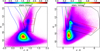 |
Fig. 1. Hess diagram of tiles b278 (left panel; l ≈ 1° and b ≈ −4°, with 0.12 ≲ E(J − Ks)≲0.67) and b320 (right panel; l ≈ 1° and b ≈ −1°, with 0.40 ≲ E(J − Ks)≲5.30). Different polygons are used to roughly highlight some of the sampled evolutionary sequences: the bright disk MS (blue polygon), the bulge RGB (black polygon), the RC (red polygon), and the blue plume of evolved disk sequence (green polygon). |
3. Methodology
Here, we describe the method that has been applied to measure color excess using RGB and RC stars in all VVV tiles, hence producing 196 individual reddening maps of 610 × 500 pixels with a field of view of roughly 1.6 deg2. In terms of figures and concrete examples, we will use a representative tile, namely b320 (0.21° < l < 1.69° and −1.56° < b < −0.35°), whose CMD is displayed in Fig. 2. This tile is especially useful as a template because of the consistently prominent and compact (in Ks) RC trail in color-magnitude it provides, extending up to J − Ks ∼ 5, which is a desirable property when attempting to define a reddening law based on the RC color-magnitude correlation.
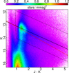 |
Fig. 2. Zoomed-in Hess diagram of the selected field b320. Solid black line follows the derived reddening vector (see text), while the dashed black box defines the polygon-region used to select the stars in the sample for the color excess calculations. Additionally, the red solid line follows Nishiyama et al. (2009) reddening law, and intersects the solid black line at (J−Ks) = 0.635, which is roughly the (J−Ks)0 of the reddening corrected RC+RGB sequence at their peak overdensity in the CMD. |
3.1. Selection of RGB and RC stars
To estimate the color excess, E(J − Ks), we take advantage of the relatively vertical sequence traced by the bulk of the RGB and RC population in the [Ks vs. (J − Ks)] plane (see Fig. 1). To isolate the RGB and RC population from the rest of the sampled stars within a given tile, we apply a color-magnitude selection in the [J − Ks] versus [Ks] CMD.
Manually and for each field, we selected all stars within a region whose color limits are set such as to include RGB and RC stars only, therefore excluding the bluer disk MS and blue plume (see blue and green boxes in Fig. 1), traced by the young (and foreground) disk stars. This isolation is key, because the foreground disk population is likely to be affected by a different reddening than the background bulge population (see Schultheis et al. 2014) and, thus, it must be excluded from the selected sample.
We defined the bright and faint limits of the selection region to vary with color following the reddening vector while containing the bulk of the RC as well as slightly brighter and fainter RGB stars, whenever this would not also include blue plume or evolved disk stars. Regarding the reddening vector, we derive it directly from the color-magnitude trend of the RC in tile b320, modeled following a similar method to the one described in Alonso-García et al. (2017). The measured reddening vector is:


In the sample field b320, the adoption of this empirical reddening vector produces a smaller dispersion in Ks for the stars in RC after correction (σKs = 0.280 mag) than when using a fixed reddening law such as Nishiyama et al. (2009) (σKs = 0.299 mag). In Fig. 2, we show the CMD of b320 with the reddening vector derived here, together with the CMD polygon-region used to define the stellar sample, and a comparison with the reddening law from Nishiyama et al. (2009). We prefer this empirical law throughout this work. After we define the selection polygon in the color-magnitude space, we pick all the stars within it and save it to a sample stellar catalog of RC and RGB stars, for which we only keep the position and color information (RC+RGB catalog).
3.2. Mapping the color of the RGB and RC sequences
We proceed by defining a grid in Galactic latitude (b) and longitude (l), which covers the area of the original field of view (in the case of VVV, roughly 1.5 × 1.2 deg2) with regularly spaced nodes; 610 in l and 500 in b, defining 305 000 pixels or nodes in the grid. This grid will define the resolution of our map, with pixel sizes < 10 arcsec. This scale is the limit at which we can trace line-of-sight variations in color of our sample RC+RGB stars.
For each node defined by the grid, we look at the closest 20 stars (a parameter henceforth referred as NAB) in the sample, based on their angular distances to the center of each pixel and filter out outliers, defined as stars whose colors are more than three median absolute deviations (MAD) from the ensemble median. The information of the remaining N stars can be reduced to a set of pairs  , where ri is the angular distance of the ith star to the pixel center and ci its J − Ks color. With this we define a set of weights wi, such that:
where rmax is the maximum from  . The weights are normalized to sum 1. These weights are mostly arbitrary, designed so that tracers near the center of the node have close-to-maximal weights while the farthest star(s) still contribute to the calculations. For instance, if we had only four tracers near the center, while the other 16 lie at the border of maximum distance to the center, rmax, then the central stars would have a contribution of about 50% by weight.
Finally, with these weights, we define four values for each node: a weighted average of the color of the N stars (ee), the weighted variance ( ), and the weighted average and maximum distance of the N stars to the center of the pixel (
 and rmax, respectively). The product of this algorithm is a cube that contains the [l, b] maps for each of those quantities. The ee values are the color excess tracers we need. Although
  could be understood as an estimate of the uncertainty in ee, here, σee is truly shown to trace the width of the color sequence distribution of the stars used in the calculation. The
  and rmax values will trace the definition of the map, that is, the smallest size of the structures the map is able to trace.
The way these maps are constructed produces an increasingly better definition the higher the stellar density of the field gets, which can reach below 20 arcsec near the Galactic plane and center. Additionally, it is important to note that we make the distinction between resolution and definition. The maps we recover here are actually an evaluation of a mosaic or tessellation defined by the data (i.e., stellar density of the RC+RGB sample) and the number of stars allowed in the calculation (NAB). This mosaic is similar to a Voronoi tessellation, but where each polygon defines the area closest to a unique combination of NAB stars, which can be smaller in size than the distance between the considered stars themselves (see Appendix A). This opens up the possibility for arbitrarily increasing the resolution (i.e., the number of nodes in the grid), which would, in principle, increase the fidelity of the evaluation, but would have no effect on the definition of the map, which is fixed by the stellar density of the RC+RGB sample and is, as a rule of thumb, the size of the smallest structures (e.g., clouds, filaments, etc) that we can trace.
3.3. Calibrated E(J − Ks) reddening maps
Once we have applied this algorithm to all 196 tiles in the VVV, we proceed to calibrate the ee values to the more useful E(J − Ks). For an internal calibration, we have taken a “whack-a-mole” approach, where given a comparison metric, we correct and calibrate outliers until the whole ensemble is consistent. In practice, we took every tile ee map and made a comparison with the ee values from the maps of their direct neighbors. That is, given that each tile has a small overlap (∼10% total area) with its immediate neighbors, we can take the mean difference between the ee values of a tile within these overlapping regions and the ee values of the respective neighbors, and provide up to four values for  (thus, only three for tiles at the border of the bulge and two for the corner fields). Since each field has a particular selection window, we expect Δee, or rather, the mean of the Δee values for each field (⟨Δee⟩), to be non-zero due to the dependence of the mean J − Ks color of the RC+RGB sequence with this selection. In a perfectly consistent ensemble, it would be possible to find a set of zero-point corrections so that all the ⟨Δee⟩ values for every field would go to 0, however, we expect to have some residual non-trivial discrepancy from the photometry (see Surot et al. 2019a), which, in practice, means that we can at best aim for a minimal or reasonable dispersion around 0. Fortunately, the concrete set of ⟨Δee⟩ values for our ensemble is already close to optimal, with only a few outliers (mostly near the center). Given the independent nature of each field, an easy way to achieve the calibration is to iteratively “hammer down” (or “up”) the strongest outlier with a zero-point correction to bring it to level with its neighbors, recalculate the ⟨Δee⟩ of the ensemble and calibrate the next strongest outlier after this correction, so that after the process is done, all the bumps are flattened and the set is more or less consistent within some dispersion. In particular, we have defined as an outlier any field whose ⟨Δee⟩ is outside of the ±2.5σ of the ensemble. This choice produces a fast convergence, where only 32 tiles are ultimately affected and where the final distribution of ⟨Δee⟩ is indistinguishable from a Gaussian distribution with mean 0 and σ = 0.007 mag.
For the absolute calibration, we used color excess values from the map of Gonzalez et al. (2012) and the improved central area from Gonzalez et al. (2018; a map referred to as G18, henceforth) as a reference, which is also based in VVV data and uses fits to the (J − Ks) color distribution of RC stars in binned fields of view and obtains a value for E(J − Ks) through a comparison with a reference RC color in Baade’s Window. With respect to the original Gonzalez et al. (2012) version, G18 boasts better resolution along the Galactic plane, as well as solving a few glitches in the central |l| ≲ 9.5° ,b ≲ 4.5° area (see Sect. 4.2 and Fig. 4). The choice for G18 is motivated by the idea that a comparison between the calibrator and this work should have minimal sources of uncertainty and the similarities listed above limit the effective difference between this work and G18 to (mostly) just resolution and photometric depth. Other maps in the literature would introduce an additional uncertainty by requiring a projection (in the case of 3D maps) or a system conversion or reddening law (in case of different passbands). Also, G18 reports a resolution of 1 arcmin in the best cases, which is the best available for its coverage. However, G18 is less sensitive to high-extinction areas than the map presented in this work. These results along with the expected abrupt changes in extinction near the plane, mean that for stars near the Galactic center and plane, we would necessarily expect to have some difference between our measurements and those in G18. For this reason, in order to obtain a straightforward zero-point calibration, we only used areas with |b| > 3°, which yielded an absolute calibration of ee − 0.605 = E(J − Ks). The field-to-field internal calibration and this global comparison essentially puts the color excess values we obtained on roughly the same reference as the one used in G18. In particular, we can compare the VVV tile containing Baade’s Window (b278, l ≈ 1° ,b ≈ −4°) and correct RC stars for both extinction by G18 and the map presented here with the reddening law from (2). In this case, the RC stars’ color standard deviation (and MAD) after correcting with this work’s map is 85% (and 83%) of the obtained from the literature extinction, while maintaining a difference in median color of only 0.004 mag.
4. Results
4.1. High spatial resolution map
In the top panel of Fig. 3, we display the whole reddening map derived in this way (it has been re-binned for plotting purposes, as the true map has a resolution of about 8540 × 7000 pixels2). In the bottom panel of the same figure, we plotted the mean definition of the map (i.e., the average size of the structure that we can trace). The best definition is near the Galactic center, where the stellar density is highest. In theory, there we could push the resolution of the map to match its definition of ∼5 arcsec. The outer bulge area maintains a more common > 1 arcmin definition.
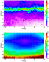 |
Fig. 3. Top panel: complete reddening map for the VVV bulge area. Bottom panel: definition of the map. |
This reddening map has already been published together with the dataset from Surot et al. (2019a), but it is also accessible through a dedicated site2 where users can upload a list of coordinates and retrieve the corresponding color excess values. Future additions to the map, including extensions to other Galactic regions, will be published on the same interface.
4.2. Comparison with the literature
To compare this work with what is already available in the literature, we use G18 as the main reference. This is preferred because (i) it is a direct comparison of the E(J − Ks) values, thus no conversion nor reddening law are necessary; and (ii) the high resolution and homogeneous coverage of G18 makes it an ideal benchmark for this work. Global comparisons with other available maps (e.g., Marshall et al. 2006; Gonzalez et al. 2012; Schultheis et al. 2014; Chen et al. 2019) are either already covered and contrasted against by G18, or would require projections or conversions to E(J − Ks) using either passband transformations or a reddening law. Both the spatial 3D distribution of reddening agents as well as the reddening law are known to change with the line of sight and we are not prepared to compensate for these nor properly characterize them given our own dataset. This severely limits the useful information such comparisons would provide. In Fig. 4, we show the uncorrected CMD for our sample field, b320, with the selection window for the RC+RGB sample used. Also shown are the extinction corrected CMD using the map from this work and a comparison with the CMD corrected using G18 map with the coefficients from Eq. (2). When using the extinction map from literature, which is roughly representative from |b| < 3° fields, it can be seen in this case that this correction produces a RC that is extended redward, suggesting that it is under-corrected, while the corrected RC from this work appears compact. This key difference arises from both the higher resolution of the maps used here and the deeper quality of the photometric dataset, thanks to which we can simply detect fainter stars (and, hence, we can measure more reddened stars). The blurred blue sequence in both panels b and c of Fig. 4 is a consequence of the over-correction for the disk stars, which mainly have a different and often much lower extinction affecting them.
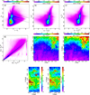 |
Fig. 4. Comparison set of the map presented in this paper and G18. Panel a: uncorrected CMD for b320, the solid line represents the selection window used to define the RC+RGB sample, as explained in the text. Panel b: reddening corrected CMD for b320, using the map in panel e (this work’s). Panel c: reddening corrected CMD for b320, using the map in panel f (G18). Both this panel and panel b use the same reddening law (see Sect. 3.1) and scale in color, so it can be appreciated the way the RC in this panel is off and slanted redward. Panel d: one-on-one comparison between the color excess values derived from this work (E(J − Ks)ee in plot) with those from G18 (E(J − Ks)G18 in plot) for the whole VVV bulge area. A color-coded density map (high density in deep red, low in magenta) with a square root filter has been used to cleanly appreciate the correspondence between G18 and this work’s color excess for low-reddening areas, while still portraying the upward trend where we find systematically higher E(J − Ks) in high extinction areas. The peculiar features near maximum and minimum E(J − Ks)G18 comes from some pixels near the Galactic center, a few high-extinction concentrations scattered around the bulge area, but mostly from a few glitches in G18 map near the Galactic plane. These are exemplified in panel g, where a small portion of the plane appears randomly jagged with constant excess areas from the original Gonzalez et al. (2012). Panel h shows the same area as panel g, but with this work’s realization. |
In panel d of Fig. 4, we also display the correspondence between the color excess values we derive here and those from G18. In low-extinction areas (and, incidentally, high-latitude) there is a general agreement. However, in mid-extinction areas, with respect to color excess from G18, we have a slight systematic underestimation of the order of 0.01–0.05 mag, while for high-extinction regions, we obtain an expected overestimation trend with respect to G18 due to the higher completeness and resolution. The few spotty discrepancies between the excesses, as well as the prominent feature of roughly constant E(J − Ks)G18, can be explained by the effect of so-called “glitches” in G18, exemplified in panel g of Fig. 4, mostly coming from challenging areas from the original Gonzalez et al. (2012) map.
Finally in Fig. 4, panels e and f display the color excess values from this work and G18 side by side in b320 region. In this setup, we can appreciate the difference in resolution and definition. The former, seen from the pixelated appearance of panel f with respect to e along with the latter, based on the not-so-evident difference in color scale, where in panel e there is an emergence of compact high-extinction regions inside the maximum extinction areas from panel f, which are otherwise unaccounted for in G18. In both cases, we can appreciate the richness of extinction structure that is present near the Galactic plane; with higher resolution and better definition, a much more complex and filamentary profile starts to emerge.
Despite the challenge noted in making comparisons with other maps in the literature, we can report that the best agreement with the map from Schultheis et al. (2014) happens with their E(J − Ks) between 6.5 and 7.0 kpc, where any further comparisons yield a systematic underestimation from our part, from a median difference at 7.0–7.5 kpc of 0.01 mag, to 0.09 mag at 10.0–10.5 kpc.
4.3. Method limitations
There are some caveats that need to be mentioned, which have a minimal effect on the quality and consistency of the derived reddening map.
4.3.1. The intrinsic colors of the RC and RGB
The observed RC and RGB colors depend not only on the reddening, but also on the metallicity of the sampled population. However, the color variation as a function of the chemical content can be predicted by stellar evolutionary models. According to the BaSTI models (Pietrinferni et al. 2013, 2014), for a 10 Gyr old population, a 1 dex change in metallicity translates into approximately 0.2 mag change in the (J−Ks) color of a RC, and about 0.13 mag for the RGB color at the same RC magnitude.
Recent spectroscopic surveys (e.g., Zoccali et al. 2017; Rojas-Arriagada et al. 2017) have found that the overall metallicity distribution of the bulge population is bimodal and spans a relatively broad but constant range, from [Fe/H] ≳ −1 dex to [Fe/H] ≲ +0.5 dex. Across the bulge area studied here, the observed field-to-field metallicity variations are due to changes in the relative fraction of these two components, metal-rich versus metal-poor stars, with the latter dominating mostly the outer regions only. However, as evident from the photometric metallicity map provided by Gonzalez et al. (2013), the mean metallicity across the bulge is confined within the range −0.6 ≲ [Fe/H] ≲ 0. Globally, this translates to ≲ 0.07 mag uncertainty due to the peak-to-valley metallicity variation across the entire bulge region. However, the metallicity variations on a field-to-field scale (i.e., within 1 deg2 areas) are considerably fewer (see Gonzalez et al. 2013), producing, hence, a much smaller uncertainty in RC color.
It is worth mentioning that different color-magnitude selections across the sampled VVV area may lead to changes in the tiles’ zero-point, (i.e., the calibration needed to transform the extracted color information to the actual color excess E(J − Ks)). However, any discrepancy is taken into account by a self-consistency check based on the overlapping areas present between adjacent tiles and then with a global zero-point correction (see Sect. 3.3).
4.3.2. Instrumental and format effects
There are two problems related to the original presentation of the data. The first is an issue that is inherited from the data images on which the photometry is based. For VIRCAM, there is a known issue with detector 16, which in practice induces a small magnitude (and color) shift in the stars that are captured on about one third of the detector. For this reddening map, the effect is ubiquitous but mostly only evident in low-reddening regions, and it appears as a regularly spaced pair of slightly higher reddening columns on the corner of each tile, aligned with the Galactic latitude axis. It is shown in the top panel of Fig. 3, for l ≲ −7°.
The second is the window effect, which affects the border of each tile. This is simply due to the discrete and modular approach to the map construction, that is, its being built of small, independent chunks. Since the algorithm uses the NAB = 20 closest stars to any grid node to estimate the mean color, the pixels close to the border, instead of selecting stars that roughly surround their center, will pick stars off to their sides and farther out in order to fulfill the NAB requirement. In practice, this means a sudden worsening of the definition, as well as the introduction of an off-center estimation of the color excess. This effect can be appreciated in the bottom panel of Fig. 3, where there is a clear net-like pattern of worse definition across the bulge area. This issue can be solved by using a coherent stellar catalog, so that for every small field of which the map is comprised, we can include stars slightly farther than the reach of the field, but without any duplicity of stars (e.g., to build the map of a field in |l| < 1° and |b| < 1°, we should include unique stars from |l| < 1.1° and |b| < 1.1° in the calculations).
4.3.3. Sensitivity of the maps: high and low ends
Since the algorithm depends on RC stars to derive an accurate tracer of E(J − Ks), if somewhere in the field, the true extinction is high enough to drive the RC stars below the detection limit, then the color excess measurement will be (silently) erroneous. Considering the limits in Surot et al. (2019a) photometry and the expected color for the RC+RGB bulge sequence, we can only detect and measure excesses below E(J − Ks)max ≲ 5.9 mag, with decreasing sensitivity as stellar crowding increases. Any area in the bulge whose true color excess is higher than this will have a quasi-random estimated value in the map. There are circumstances that can either mitigate and aggravate this issue. If there is even a moderate reddening in the foreground (i.e., affecting the near disk stars) then the blue plume or the young disk MS itself can be pushed into the selection polygon and be considered in the RC+RGB sample as color excess tracers. In this scenario, an extremely high extinction area will suddenly appear as a very low extinction window. A most dramatic example of this can be observed in Fig. 3, in a 16 × 10 arcmin2 window centered at (l, b)≈(8.48° , − 0.28° ), where it appears there are only a few bulge stars and an extincted disk sequence. Here the code reports E(J − Ks)≈2, where it should be higher than 4 mag. On the other hand, if red stars still dominate the area of high reddening, then what is more likely to happen is that the density of tracers will drastically drop, substantially worsening the definition of the map near that area but otherwise still producing a high extinction estimation of the E(J − Ks) there, in a fashion similar to how saturation and non-linear responses affect photometric images; plateauing about the extinction threshold.
A final caveat comes from the high latitudes fields, and coincidentally, low extinction. In these regions, we had to pay special attention to not include within the CMD polygon the local K- and M-dwarfs sequence (mentioned in Surot et al. 2019a; Saito et al. 2012) at (J − Ks)≈0.8, whose bright stars can intrude into the selection polygon. Although this sequence potentially exists in all the bulge area, the considerably low bulge-star density on these high latitude areas exacerbates the effect these otherwise rare stars have on the E(J − Ks) estimations. In general, in this region we have an overall reduced good-to-bad stellar ratio, where a good star is simply a RC+RGB bulge star and a bad one is neither (including artifacts).
5. Discussion and conclusions
In this paper, we detail the methodology we have used to derive a sub-arcmin resolution E(J − Ks) map for the whole VVV bulge area, within |l|≲10° and −10° ≲b ≲ 5° (see Fig. 3). With this map, we have found agreement with G18 map (also based in VVV data and with the same filters) in low extinction areas, but we also found significant discrepancies in the highest extinction areas. We argue that for these very high extinction areas, previous studies lack both the photometric completeness and resolution to both observe and identify extremely reddened stars and to discern sub-arcmin sized very-high extinction patches. Regardless of the numerical discrepancy, we maintain an excellent agreement with the general structure tracing of the reddening agents in the bulge area.
The top panel of Fig. 3 displays the whole extinction map, where we can appreciate how faint and expansive structures pop up from the granular background for b < −6°, while the general trend going inward to |b| < 4° appears to be a superposition of threads and thin filaments, up until the Galactic plane area shows a generally tangled, bubbly, and clumpy distribution. With this level of detail, this map proves that if we want to study and understand the stars on the Galactic plane and center, especially bulge stars, we must consider not only prohibitive extinctions, but also, high levels of variability and structured profiles of dust and gas along the line of sight on small (< 1′) scales. A small and elusive property of this map and method is that they can also pick up small color variations produced by clustered stars, which are represented by very localized and sudden changes in color excess (usually bluer than the background) that highlight these objects. In practice, due to this phenomenon, foreground clusters visibly pop-up from the background extinction.
As mentioned in Sect. 3, we calculate the width of the color distribution of the sample used to procure the color excesses. We selected this quantity because the color width is also a proxy for optical depth in the line-of-sight. Thanks to the small bin sizes (∼9 arcsec or ∼350 pc from an 8 kpc bulge), we can isolate large-scale line-of-sight excess variations and know, aside from a baseline dispersion of the sequence, due to actual population diversity and photometric effects, that whatever scatter in color we observe must come from the dust and gas distribution itself. Additionally, this color width can be taken at face value for simulations and artificial stellar population syntheses in cases where the use of the proper photometric data is either prohibitive or too expensive. That said, this same width can be used as a scaled uncertainty estimate of E(J − Ks), which will be provided in the dataset.
Also, we can make note of the next layer of information added to the map, namely, the definition. In panel b of Fig. 3, we have mapped this value to show how quickly it can go below the 1 arcmin mark and we can even see that in the most dense areas, this value is as low as < 5 arcsec, which means that the resolution we adopted is, in principle, insufficient to properly characterize those areas. In fact, using these smaller bin sizes increases the maximum color excess values we recover, continuing the trend we have pointed out before, namely, that with higher and higher resolutions come stronger peaks in the extinction distribution profile. However, having < 2 arcsec resolution maps inside this highest density area only gives incremental benefits, which need to be paired with better photometry and more information so that they may be fully taken advantage of.
The accurate definition of the differential extinction in bulge fields is key for an adequate synthetic population analysis (Surot et al. 2019b, and references therein). In similar works and anything relating to star formation history (SFH) reconstruction via CMD fitting, inadequate solutions for the differential extinction of the field under study could have detrimental effects, from significantly reducing the information the fit can provide, given that a color dispersion product of a mischaracterization of the extinction could be interpreted as a dispersion in metallicity or age, to rendering such a study impossible in all but small consistent extinction windows, which usually also implies either a low extinction area away from the plane or a far too limited sample of the bulge stars in these sparse windows. As mentioned in Sect. 3.3, even in relatively low extinction regions, this map reduces the dispersion in the RC magnitudes with respect to G18 by ∼20% and, as presented in Fig. 4, it can visibly improve the corrections of fields near the plane, most evidently in the color distribution of the RC locus. For instance, the central tile b333 (−1.25 < l < 0.23 and −0.46 < b < 0.75) shows an improvement over the standard deviation from the (J − Ks)0 distribution of its RC area, from 0.46 mag with G18 to 0.24 mag (∼46% reduction) in this work. This improvement in extinction determination, paired with a decontamination procedure can make it possible to carry out SFH studies on the plane, which would otherwise be inconclusive due to any improperly handled extinction. In addition, having a solid determination of extinction is also important for target selection in spectroscopic surveys, which rely on photometric properties related to the desired stellar parameters (e.g., photometric effective temperature, classification, etc.) and, in particular, upcoming spectroscopic facilities (e.g., MOONS – Cirasuolo et al. 2011; 4MOST – de Jong et al. 2019), which will be able to target thousands of stars across the bulge, benefiting from a reliable and accurate extinction on the plane for this purpose.
This particular version of the map has was already used in Surot et al. (2019b) and incorporated into the MW-BULGE-PSPHOT dataset (Surot et al. 2019a), but it is also accessible through a dedicated site3 where users can upload a list of coordinates and retrieve the corresponding color excess values. Future additions to the map, including extensions to other Galactic regions, will be published on the same interface.
Acknowledgments
FS acknowledges financial support through the grants (AEI/FEDER, UE) AYA2017-89076-P, as well as by the Ministerio de Ciencia, Innovación y Universidades (MCIU), through the State Budget and by the Consejería de Enconomía, Industria, Comercio y Conocimiento of the Canary Islands Autonomous Community, through Regional Budget. EV acknowledges the Excellence Cluster ORIGINS Funded by the Deutsche Forschungsgemeinschaft (DFG, German Research Foundation) under Germany’s Excellence Strategy – EXC-2094 – 390783311. Support for M.Z. and D.M. is provided by the BASAL CATA Center for Astrophysics and Associated Technologies through grant PFB-06, and the Ministry for the Economy, Development, and Tourism’s Programa Iniciativa Científica Milenio through grant IC120009, awarded to the Millenium Institute of Astrophysics (MAS). M.Z. acknowledges support from FONDECYT Regular 1191505. D.M. acknowledges support from FONDECYT Regular 1170121. S.H. and E.S. acknowledge grant 309290 form IAC and grant AYA2013-42781P from the Ministry of Economy and Competitiveness of Spain.
References
- Alonso-García, J., Minniti, D., Catelan, M., et al. 2017, ApJ, 849, L13 [Google Scholar]
- Alonso-García, J., Saito, R. K., Hempel, M., et al. 2018, A&A, 619, A4 [NASA ADS] [CrossRef] [EDP Sciences] [Google Scholar]
- Benjamin, R. A., Churchwell, E., Babler, B. L., et al. 2003, PASP, 115, 953 [NASA ADS] [CrossRef] [Google Scholar]
- Chen, B.-Q., Huang, Y., Yuan, H.-B., et al. 2019, MNRAS, 483, 4277 [NASA ADS] [CrossRef] [Google Scholar]
- Cirasuolo, M., Afonso, J., Bender, R., et al. 2011, Messenger, 145, 11 [Google Scholar]
- de Jong, R. S., Agertz, O., Berbel, A. A., et al. 2019, Messenger, 175, 3 [Google Scholar]
- Dutra, C. M., Santiago, B. X., Bica, E. L. D., & Barbuy, B. 2003, MNRAS, 338, 253 [NASA ADS] [CrossRef] [Google Scholar]
- Epchtein, N. 1998, in New Horizons from Multi-Wavelength Sky Surveys, eds. B. J. McLean, D. A. Golombek, J. J. E. Hayes, & H. E. Payne, IAU Symp., 179, 106 [Google Scholar]
- Gonzalez, O. A., Rejkuba, M., Zoccali, M., et al. 2012, A&A, 543, A13 [NASA ADS] [CrossRef] [EDP Sciences] [Google Scholar]
- Gonzalez, O. A., Rejkuba, M., Zoccali, M., et al. 2013, A&A, 552, A110 [NASA ADS] [CrossRef] [EDP Sciences] [Google Scholar]
- Gonzalez, O. A., Minniti, D., Valenti, E., et al. 2018, MNRAS, 481, L130 [NASA ADS] [CrossRef] [Google Scholar]
- Gosling, A. J., Bandyopadhyay, R. M., & Blundell, K. M. 2009, MNRAS, 394, 2247 [NASA ADS] [CrossRef] [Google Scholar]
- Lawrence, A., Warren, S. J., Almaini, O., et al. 2007, MNRAS, 379, 1599 [NASA ADS] [CrossRef] [MathSciNet] [Google Scholar]
- Marshall, D. J., Robin, A. C., Reylé, C., Schultheis, M., & Picaud, S. 2006, A&A, 453, 635 [NASA ADS] [CrossRef] [EDP Sciences] [Google Scholar]
- Minniti, D. 2016, Galactic Surveys: New Results on Formation, Evolution, Structure and Chemical Evolution of the Milky Way, 10 [Google Scholar]
- Minniti, D., Lucas, P. W., Emerson, J. P., et al. 2010, New Astron., 15, 433 [Google Scholar]
- Minniti, D., Saito, R. K., Gonzalez, O. A., et al. 2018, A&A, 616, A26 [NASA ADS] [CrossRef] [EDP Sciences] [Google Scholar]
- Nataf, D. M., Gonzalez, O. A., Casagrande, L., et al. 2016, MNRAS, 456, 2692 [NASA ADS] [CrossRef] [Google Scholar]
- Nishiyama, S., Tamura, M., Hatano, H., et al. 2009, ApJ, 696, 1407 [NASA ADS] [CrossRef] [Google Scholar]
- Pietrinferni, A., Cassisi, S., Salaris, M., & Hidalgo, S. 2013, A&A, 558, A46 [NASA ADS] [CrossRef] [EDP Sciences] [Google Scholar]
- Pietrinferni, A., Molinaro, M., Cassisi, S., et al. 2014, Astron. Comput., 7, 95 [NASA ADS] [CrossRef] [Google Scholar]
- Rojas-Arriagada, A., Recio-Blanco, A., de Laverny, P., et al. 2017, A&A, 601, A140 [NASA ADS] [CrossRef] [EDP Sciences] [Google Scholar]
- Saito, R. K., Minniti, D., Dias, B., et al. 2012, A&A, 544, A147 [NASA ADS] [CrossRef] [EDP Sciences] [Google Scholar]
- Saito, R. K., Minniti, D., Benjamin, R. A., et al. 2020, MNRAS, 494, L32 [CrossRef] [Google Scholar]
- Schultheis, M., Ganesh, S., Simon, G., et al. 1999, A&A, 349, L69 [NASA ADS] [Google Scholar]
- Schultheis, M., Sellgren, K., Ramírez, S., et al. 2009, A&A, 495, 157 [NASA ADS] [CrossRef] [EDP Sciences] [Google Scholar]
- Schultheis, M., Chen, B. Q., Jiang, B. W., et al. 2014, A&A, 566, A120 [NASA ADS] [CrossRef] [EDP Sciences] [Google Scholar]
- Skrutskie, M. F., Cutri, R. M., Stiening, R., et al. 2006, AJ, 131, 1163 [NASA ADS] [CrossRef] [Google Scholar]
- Surot, F., Valenti, E., Hidalgo, S. L., et al. 2019a, A&A, 623, A168 [NASA ADS] [CrossRef] [EDP Sciences] [Google Scholar]
- Surot, F., Valenti, E., Hidalgo, S. L., et al. 2019b, A&A, 629, A1 [NASA ADS] [CrossRef] [EDP Sciences] [Google Scholar]
- Zoccali, M., Vasquez, S., Gonzalez, O. A., et al. 2017, A&A, 599, A12 [NASA ADS] [CrossRef] [EDP Sciences] [Google Scholar]
Appendix A: Higher order Voronoi diagrams
One way to understand a Voronoi diagram is by thinking of each polygon-cell in the tessellation, as the locus of points on the plane closest to any one particular seed-generator point. This is a quite useful way to represent properties of a field whose probes are distributed irregularly on the phase space. With this in mind, we can define tessellations of the phase space based on sets of unique combinations of n seed points, that is, the cells in this partition would rather represent the loci of points closest to a particular set of n seeds. This representation would then be useful whenever the field property depends on several probes, as is the case of the excess values estimated here.
In Fig. A.1, we depict several Voronoi diagrams, corresponding to n = 1, 2, 4, and 8 for the same toy model of uniformly distributed points with x, y ∈ [ − 1.5, 1.5]. For n = 1, it is the familiar representation of a Dirichlet tessellation, where the seed points are all contained in their respective cells and vice versa. However, for n > = 2, the polygons start to become generally smaller the higher n is, with increasingly more polygons containing no seed points (and some containing more than one). While for a standard Voronoi diagram (n = 1) the size or area of its cells is simply a reflection of the separation of the seeds, for higher order tessellations, the dimensions of these cells are generally smaller than the distance between the seeds. For this work, in particular, we have a n = 20 and each seed is a probe RC+RGB star. Then each tiny cell provides a uniquely defined ee value, essentially defining an ee field, which varies on scales that are much smaller than typical stellar probe separations. The maps we provide here, rather than serving as an interpolation, are a relatively sparse evaluation of this true field, on regularly spaced nodes. In general, these cells are bigger than the separation of the nodes, so no information is wasted. However, near the center, the probe density is so high that even this typical node separation of ≲10 arcsec is too big for an extensive evaluation of the field and, thus, it could, in principle, be reduced to probe the tessellation more effectively. No particular improvement would be gained from this, however, because in these regions we appear to be limited more by depth than line-of-sight variations.
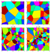 |
Fig. A.1. Voronoi diagrams of orders 1, 2, 4, and 8 of a uniformly distributed (x, y) toy seed points set where x ∈ [ − 1.5, 1.5] and y ∈ [ − 1.5, 1.5]. Each panel only shows x ∈ [ − 1, 1],y ∈ [ − 1, 1] to avoid window effects. The toy set is the same for each panel, but the order is different (n = 1, 2, 4, and 8, shown on top of each panel). The seed points are shown as small black circles, while each cell is randomly colored in the background and their borders delimited by solid black lines. |
All Figures
|
Fig. 1. Hess diagram of tiles b278 (left panel; l ≈ 1° and b ≈ −4°, with 0.12 ≲ E(J − Ks)≲0.67) and b320 (right panel; l ≈ 1° and b ≈ −1°, with 0.40 ≲ E(J − Ks)≲5.30). Different polygons are used to roughly highlight some of the sampled evolutionary sequences: the bright disk MS (blue polygon), the bulge RGB (black polygon), the RC (red polygon), and the blue plume of evolved disk sequence (green polygon). |
| In the text | |
|
Fig. 2. Zoomed-in Hess diagram of the selected field b320. Solid black line follows the derived reddening vector (see text), while the dashed black box defines the polygon-region used to select the stars in the sample for the color excess calculations. Additionally, the red solid line follows Nishiyama et al. (2009) reddening law, and intersects the solid black line at (J−Ks) = 0.635, which is roughly the (J−Ks)0 of the reddening corrected RC+RGB sequence at their peak overdensity in the CMD. |
| In the text | |
|
Fig. 3. Top panel: complete reddening map for the VVV bulge area. Bottom panel: definition of the map. |
| In the text | |
|
Fig. 4. Comparison set of the map presented in this paper and G18. Panel a: uncorrected CMD for b320, the solid line represents the selection window used to define the RC+RGB sample, as explained in the text. Panel b: reddening corrected CMD for b320, using the map in panel e (this work’s). Panel c: reddening corrected CMD for b320, using the map in panel f (G18). Both this panel and panel b use the same reddening law (see Sect. 3.1) and scale in color, so it can be appreciated the way the RC in this panel is off and slanted redward. Panel d: one-on-one comparison between the color excess values derived from this work (E(J − Ks)ee in plot) with those from G18 (E(J − Ks)G18 in plot) for the whole VVV bulge area. A color-coded density map (high density in deep red, low in magenta) with a square root filter has been used to cleanly appreciate the correspondence between G18 and this work’s color excess for low-reddening areas, while still portraying the upward trend where we find systematically higher E(J − Ks) in high extinction areas. The peculiar features near maximum and minimum E(J − Ks)G18 comes from some pixels near the Galactic center, a few high-extinction concentrations scattered around the bulge area, but mostly from a few glitches in G18 map near the Galactic plane. These are exemplified in panel g, where a small portion of the plane appears randomly jagged with constant excess areas from the original Gonzalez et al. (2012). Panel h shows the same area as panel g, but with this work’s realization. |
| In the text | |
|
Fig. A.1. Voronoi diagrams of orders 1, 2, 4, and 8 of a uniformly distributed (x, y) toy seed points set where x ∈ [ − 1.5, 1.5] and y ∈ [ − 1.5, 1.5]. Each panel only shows x ∈ [ − 1, 1],y ∈ [ − 1, 1] to avoid window effects. The toy set is the same for each panel, but the order is different (n = 1, 2, 4, and 8, shown on top of each panel). The seed points are shown as small black circles, while each cell is randomly colored in the background and their borders delimited by solid black lines. |
| In the text | |
Current usage metrics show cumulative count of Article Views (full-text article views including HTML views, PDF and ePub downloads, according to the available data) and Abstracts Views on Vision4Press platform.
Data correspond to usage on the plateform after 2015. The current usage metrics is available 48-96 hours after online publication and is updated daily on week days.
Initial download of the metrics may take a while.