| Issue |
A&A
Volume 644, December 2020
|
|
|---|---|---|
| Article Number | A138 | |
| Number of page(s) | 12 | |
| Section | Stellar structure and evolution | |
| DOI | https://doi.org/10.1051/0004-6361/202038098 | |
| Published online | 11 December 2020 | |
Inferring the internal structure of γ Doradus variables from Rossby modes
Extension of the ν − √Δν diagram
1
Department of Astronomy, School of Science, The University of Tokyo, 7-3-1 Hongo, Bunkyo-ku, Tokyo 113-0033, Japan
e-mail: takata@astron.s.u-tokyo.ac.jp
2
LESIA, Observatoire de Paris, PSL Research University, CNRS, Sorbonne Universités, UPMC Univ. Paris 06, Univ. Paris Diderot, Sorbonne Paris Cité, 5 place Jules Janssen, 92195 Meudon, France
3
Astronomical Institute, Graduate School of Science, Tohoku University, Sendai 980-8578, Japan
4
IRAP, Université de Toulouse, CNRS, UPS, CNES, 14 avenue Édouard Belin, 31400 Toulouse, France
5
DTU Space, National Space Institute, Technical University of Denmark, Elektrovej 328, 2800 Kgs. Lyngby, Denmark
6
Stellar Astrophysics Centre, Department of Physics and Astronomy, Aarhus University, Ny Munkegade 120, 8000 Aarhus C, Denmark
7
Observatoire de Genève, Université de Genève, 51 Ch. Des Maillettes, 1290 Sauverny, Switzerland
Received:
6
April
2020
Accepted:
9
October
2020
A unique type of oscillation modes has recently been identified in γ Doradus variables. These low-frequency modes are called Rossby modes (or r modes) because they consist of Rossby waves in each spherical layer. These waves are characterised by toroidal motions that are restored by the latitudinal variation in the Coriolis force. The horizontal oscillations are weakly coupled in the radial direction. We show that these modes can be used to probe the interior of the stars. The method of the ν − √Δν diagram, which has originally been developed to analyse another type of modes, Kelvin g-modes (or prograde sectoral g-modes), is extended to take Rossby modes into account. We first show based on a theoretical model and then on two stars, KIC 3240967 and KIC 12066947, that the method can be adapted to Rossby modes straightforwardly. In addition, we demonstrate that simultaneous analysis of Kelvin and Rossby modes results in (1) smaller uncertainties in the internal rotation rate and the characteristic period of gravity modes, and (2) a substantial reduction of the correlation between the estimates of the two parameters.
Key words: asteroseismology / stars: oscillations / stars: rotation / methods: data analysis
© ESO 2020
1. Introduction
Recent space missions for exoplanet study, such as CoRoT1 (Baglin et al. 2006), Kepler (Borucki et al. 2010), and TESS2 (Ricker et al. 2014), have brought (and still bring) dramatic changes in asteroseismology, the study of the interior of stars based on their oscillation. The change can be considered to be twofold from an observational point of view. On the one hand, high-precision photometric data have unambiguously revealed oscillations with tiny amplitudes. Typical examples include solar-like oscillations in a large number of main-sequence and evolved stars (e.g. Chaplin & Miglio 2013). On the other hand, long-term continuous observations have clearly resolved complicated spectra of oscillation frequencies. One of the most successful cases is found in γ Doradus (γ Dor) stars (e.g. Van Reeth et al. 2015). This is a class of intermediate-mass main-sequence oscillators. They benefit from continuous observations from space because they have many oscillation periods of the order of one day, which show serious aliasing problems when they are observed from ground.
The observations from space have also strongly affected theoretical studies. Before the space age, when the data quality was poor, studies of stellar oscillations were often motivated by theoretical interest. Some oscillation modes of special physical characters have been discussed without regard to whether they are detected in real stars. Two examples can be listed here: mixed modes in evolved stars (Osaki 1975), and Rossby modes (or r-modes) in rotating stars (Papaloizou & Pringle 1978). The space missions did indeed detect both of these modes (Bedding et al. 2010; Beck et al. 2011; Van Reeth et al. 2016; Saio et al. 2018), which stimulates fresh theoretical interests to establish asteroseismology. Mixed modes have a dual character of acoustic and gravity modes because they consist of internal gravity waves in the dense central core and acoustic waves in the extended envelope. They play a major role in red giant seismology (e.g. Bedding et al. 2011; Mosser et al. 2011; Beck et al. 2012). Rossby modes can be regarded as global counterparts of Rossby waves, which are known from meteorology (Rossby 1939; Gill 1982). The phase of these waves propagates in the opposite direction to the rotation in the co-rotating frame, showing toroidal motions in each spherical layer of stars. The horizontal propagation can be understood based on the conservation of the potential vorticity. The latitudinal variation in the Coriolis force serves as the restoring force. These modes are the second most common modes in γ Dor stars after Kelvin g-modes (or prograde sectoral g-modes), which are global manifestations of equatorial Kelvin waves (Thomson 1880; Gill 1982). The two types of modes can explain most of the detected modes (e.g. Li et al. 2020). The dominance of these modes, particularly in rapid rotators, can probably be understood by the smaller geometrical cancellation of photometric signals over the visible hemisphere than the other types of modes, but the weaker radiative damping caused by the longer horizontal wavelengths could also contribute. It has been claimed that Rossby modes are also found in other types of stars (Saio 2018).
The oscillation periods of γ Dor stars are much longer than the dynamical timescale at the surface of about an hour, while their rotation has periods of the same order as the oscillation. Because oscillations like this are thought to be strongly affected by rotation, they provide us with an ideal opportunity to study the internal rotation and structure of these stars. Takata et al. (2020) (hereafter, Paper I) developed a method for extracting the following two parameters from the frequencies of Kelvin g-modes: the (average) rotation frequency νrot and the characteristic period P0 of gravity-mode oscillations. We note that P0 can be regarded as a measure of the evolutionary stage because it monotonically decreases with stellar evolution. The main purpose of the paper is to revise the method so that Rossby modes are included.
Helioseismology has shown that it is important to consider multiple types of modes to infer the stellar structure accurately (e.g. Gough 1985) because different types of modes represent different aspects of the structure. It is essential to use acoustic modes in a wide range of spherical degrees that have different inner turning points to constrain the profile of the sound speed from the near-surface layers to the deep interior of the Sun. The detection of only a few gravity modes in addition to a large number of acoustic modes is expected to significantly improve the inversion results of the rotation and the sound speed near the centre. Similarly, the rotation rates of the core and envelope of evolved stars have been estimated from mixed modes with various degrees of mixture of acoustic and gravity modes (e.g. Deheuvels et al. 2012, 2014). In the case of (slowly rotating) main-sequence hybrid pulsators of δ Sct and γ Dor type, the rotation rates have been determined independently in the envelope and the core from acoustic and gravity modes, respectively (Kurtz et al. 2014; Saio et al. 2015; Schmid et al. 2015). The inferred contrasts in the rotation rates between the core and the envelope give valuable information about the problem of angular momentum transport inside stars. We discuss whether a similar improvement can be observed in the seismic inferences of γ Dor stars by combining Rossby modes with Kelvin g-modes.
The structure of the paper is as follows: we extend in Sect. 2 the method of the  diagram to take not only Kelvin g-modes into account, but Rossby modes as well. The extended method is validated based on a theoretical model in Sect. 3. The method is applied to real stars in Sect. 4. Section 5 is devoted to the discussion and conclusion.
2. Method
The fundamental formula of our analysis is the asymptotic expression of the oscillation frequencies in the traditional approximation of rotation (Eckart 1960). This is generally known to be a good approximation for low-frequency oscillations in rotating stars, which consist of waves with short wavelengths in the radial direction (e.g. Ballot et al. 2012; Ouazzani et al. 2017). The details are described in Paper I, therefore we only give a concise description of the framework here. The period in the co-rotating frame is provided by
in which the meanings of the symbols are given as follows: νco is the oscillation frequency in the co-rotating frame, n is the radial order of oscillation modes (n < 0 and |n| ≫ 1), α is the phase changes introduced at the inner and outer boundaries of the propagation region, P0 is the characteristic period of the gravity modes, and λ is the eigenvalue of the Laplace tidal equation. If the rotation frequency νrot is not constant but weakly dependent on the distance from the centre, r, the co-rotating frame should be interpreted as the frame that rotates with the weighted average over the propagation region (G),
where N is the Brunt–Väisälä frequency. We do not consider the case of strong differential rotation in this paper. The definition of P0 is given by
In the limit of no rotation, the frequencies of high-order g-modes with spherical degree ℓ are evenly spaced in period with  . We adopt the conventions that νrot, νco, and the oscillation frequency in the inertial frame, ν, are all positive, and that the azimuthal order m is positive (negative) for prograde (retrograde) modes. These quantities are related to each other by
We developed in Paper I the method of the  diagram, in which Δν means the difference between the two adjacent frequencies, to estimate νrot and P0 from the observed frequencies of Kelvin g-modes. Its main point is to reduce the problem of non-linear fitting to that of iterative linear fitting, which is easier to understand and far easier to solve. This reduction is made possible because λ of Kelvin g-modes with a given m is nearly independent of the spin parameter, which is defined by

We observe in Fig. 1 that

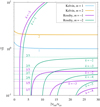 |
Fig. 1. Profiles of |

Rossby modes share a similar property because

(cf. Townsend 2003). We note that the index k is related to the structure of the corresponding eigenfunction (Hough function) of the Laplace tidal equation (cf. Lee & Saio 1997) such that for retrograde modes with k ≤ −1, the number of nodes is equal to |k| and |k+2| for odd and even |k|, respectively. In particular, the Hough function associated with an even (odd) value of |k| is symmetric (anti-symmetric) with respect to the equator.
We may therefore construct the  diagram for these Rossby modes in just the same way as Kelvin g-modes in Paper I. If a list of frequency {νi} with the same m and k is given in ascending order, we can derive the approximate relation,
for |n| ≫ 1 or s ≫ 1. Here we have introduced Δiν = νi + 1 − νi, Δin = |ni + 1−ni|, and  , in which ni stands for the radial order of the mode with the i-th frequency. Equation (8) means that there is a linear relation between
  and
and  . This is different from the corresponding relation for Kelvin g-modes (Eq. (10) of Paper I) only in the first factor on the left-hand side,
  , which is missing in the latter. The negative sign on the left-hand side arises because the frequency difference of two adjacent Rossby modes is smaller for higher frequencies, which is opposite to the case of Kelvin g-modes. The right-hand side is accordingly negative. This is because of νco < νrot for Rossby modes (e.g. Saio et al. 2018) and Eq. (4), which is reduced to

While the linear relation given by Eq. (8) is valid only for Rossby modes in the limit of s ≫ 1, we choose to use the more general non-linear relation in this analysis (cf. Eq. (10)).
As in the case of Kelvin g-modes in Paper I, we may generalise Eq. (8) to take the Kelvin and Rossby modes into account as
in which xi and yi are defined by

and
respectively. We have introduced fi in Eq. (12), which is given by
![$$ \begin{aligned} f_i \left(\nu _{\mathrm{rot}}\right) = \left[ \frac{-1}{\left|m\right|\Delta _i\nu } \Delta _i \left( \frac{\sqrt{\lambda }}{\nu _{\mathrm{co}}} \right) \right]^{\frac{1}{2}} \left( \nu _{i+\frac{1}{2}} - \left|m\right| \nu _{\mathrm{rot}} \right) , \end{aligned} $$](/articles/aa/full_html/2020/12/aa38098-20/aa38098-20-eq23.gif)
to consider the deviations from the asymptotic expressions of  (Eqs. (6) and (7)) and those from the linearisation relation, Δiν−1 ≈ −ν−2Δiν. Because fi depends on νrot and the frequency of each mode, Eq. (10) is a non-linear equation. As νrot → ∞, fi(νrot) is asymptotically equal to
When we correctly identify m, k, and Δin, we can develop the procedure of iterative linear fitting to estimate νrot and P0 from the frequency list {νi} based on Eq. (10) (cf. Paper I). The initial values of fi can be set to f0 independent of i (and hence frequency). We stress, however, that fi(νrot) is updated with a new value of νrot after each iteration based on Eq. (13), which depends on νi and νi + 1. The uncertainties in the estimated parameters can be evaluated with the method described in Appendix A of Paper I. We note that these uncertainties should be considered as formal because the systematic errors in Eq. (10) are not taken into account.
Figure 1 shows that the case of k = −1 is exceptional because  does not tend to any constant, but

These were called retrograde Yanai modes by Townsend (2003), and are composed of more gravity waves than Rossby waves when the rotation is rapid (s ≫ 1). Because these modes are rarely detected and resolved even in the Kepler data (cf. Saio et al. 2018; Li et al. 2020), we do not consider them to estimate νrot and P0.
3. Tests based on an evolutionary model
We applied the method of the  diagram to a typical theoretical model of γ Dor stars. The model is the same as Model A of Christophe et al. (2018) and Paper I, which has a mass of 1.86 M⊙ and νrot = 7 μHz. We first used the frequencies of Rossby modes alone, and then used those of both Kelvin and Rossby modes.
3.1. Analysis based on Rossby modes alone
The frequencies of Rossby modes were computed with the ACOR oscillation code (Ouazzani et al. 2012, 2015) for m = −1, k = −2 and the radial order from n = −21 to −99. The corresponding range of the spin parameter is roughly between s = 7 and 20. The  diagram is shown in Fig. 2, and the estimates for νrot and P0 are given in rows 4 and 5 of Table 1.
 |
Fig. 2. Diagram of ν vs. |


Estimates of νrot and P0 for the evolutionary model of a γ Dor star (Model A of Christophe et al. 2018).
Figure 2 shows that the open blue circles are not aligned on a straight line, but rather on a concave curve. This is because the asymptotic relations of Eqs. (7) and (8) for m = −1 and k = −2 are inaccurate particularly for s ≲ 10, as Fig. 1 shows. As a result, the fitted line of iteration 1 (the dashed blue line) gives νrot = 7.66 μHz and P0 = 1.57 × 10³ s, which are different from the true values by 9% and −66%, respectively. Although the first iteration provides such poor results, the procedure converges after 15 iterations when the relative differences in the estimated νrot and P0 between two successive iterations become less than 10−4. We note that s is smaller for lower frequency modes in Fig. 2, and the deviation of fi(νrot) from f0 is accordingly larger. For the converged estimate of νrot, the correction factor fi/f0 is equal to 1.47 for the lowest frequency pair, and it monotonically decreases until it reaches 1.01 for the highest frequency pair. The corrected values yi for the converged estimate of νrot are shown in Fig. 2 as small open orange circles, which are almost perfectly aligned with the fitted (solid) line. We thus obtain νrot = 7.032 ± 0.002 μHz and P0 = (4.47±0.01) × 103 s, which agree with the true values within 0.5% and 2%, respectively. We note that these differences from the true values are larger than the estimated formal uncertainties, which are 0.03% and 0.3% for νrot and P0, respectively. The correlation coefficient a (cf. Eq. (A.29) of Paper I) between the estimates of νrot and P0 is nearly equal to −1. This high anti-correlation can be understood from Fig. 2. All of the open circles are distributed in the lower left side of the abscissa intercept (open square) of the best-fit line (solid line). When the intercept (νrot) is slightly moved to the right side and the fitting process is repeated under this condition, the fitted line should have a shallower slope ( ) because the line must roughly go through the centre of distribution of the open circles. Thus, the increase in νrot must result in the decrease in P0.
In order to determine how robust the iterative procedure is, we performed experiments by discarding high-frequency components in the list step by step. When we used only frequencies below 5.9 μHz, which corresponds to s < 12.5, the procedure still converged after 78 iterations. The converged values of νrot and P0 are 7.020 ± 0.002 μHz (0.6066 ± 0.0002 d−1) and (4.52 ± 0.01) × 103 s, respectively. These are marginally closer to the true values in the last row of Table 1 than the values in row 5 of Table 1, which were obtained by taking all the frequencies into account. The reason for these differences is that the accuracy of Eq. (1) depends on the frequency range. In other words, treatment beyond the traditional approximation of rotation in the asymptotic regime is necessary to discuss this problem further (cf. Sect. 5). On the other hand, the procedure fails to converge even after 100 iterations when the upper limit is set at 5.8 μHz, which implies s < 11.5. It is thus essential to include high frequencies in the analysis when Rossby modes alone are used. We confirmed that the procedure without Rossby modes above 5.8 μHz converges successfully again when we take Kelvin g-modes into account (cf. Sect. 3.2).
We reproduce the results of Paper I based on Kelvin g-modes in rows 7 and 8 of Table 1. Comparing these with the case of Rossby modes, we find the following: (a) the number of iteration required for convergence is much larger for Rossby modes (15) than Kelvin modes (5), (b) the converged value of νrot is higher (lower) by less than 1% than the true value for Rossby (Kelvin) modes, (c) those of P0 are shorter by 2% than the true value for both types of modes, and (d) the estimates of νrot and P0 are highly anti-correlated (correlated) with each other for Rossby (Kelvin) modes. Point (a) is because the deviation from the asymptotic relation of  (cf. Eqs. (6) and (7)) for low values of the spin parameter is more significant for Rossby modes than for Kelvin modes, as shown in Fig. 1. The range of fi/f0 is 1.002–1.036 for Kelvin g-modes, and it is 1.01–1.47 for Rossby modes.
3.2. Analysis based on both Kelvin and Rossby modes
In rows 10 and 11 of Table 1 we provide the results based on both Kelvin and Rossby modes. The corresponding  diagram is depicted in Fig. 3. The points we find can be summarised as follows:
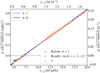 |
Fig. 3. Same as Fig. 2, but based on both Kelvin and Rossby modes, which are denoted by open red and blue circles, respectively. Small open orange circles represent |

1. The differences in the converged values of νrot and P0 from the true values are reduced to 0.2% and 0.3%, respectively.
2. The number of iterations required for convergence (6) is much smaller than in the case of Rossby modes (15), and it is similar to the case of Kelvin modes (5).
3. The formal uncertainty of 0.3% in the estimate of νrot is similar to the case of Rossby modes, and smaller by several factors than in the case of Kelvin modes. The uncertainty of 0.07% for P0 is smaller by a few factors than in the separate analyses of Rossby and Kelvin modes.
4. Even the outputs of the first iteration (νrot = 6.91 μHz and P0 = 4.31 × 10³ s) give reasonably good estimates of the true values (νrot = 7 μHz and P0 = 4.579 × 10³ s). This can be understood as (partial) cancellation. When Rossby (or Kelvin) modes alone are analysed separately, the first iteration gives larger (or smaller) νrot and smaller (or larger) P0 than the true vales. These opposite differences come from the behaviour of  : it increasingly (decreasingly) approaches the asymptotic value given by Eq. (7) (Eq. (6)) for Rossby (Kelvin) modes, as shown in Fig. 1.
5. The low correlation coefficient of 0.27 between the estimates of νrot and P0 indicates the significant improvement from the cases that use Rossby or Kelvin modes alone. While the estimates are highly anti-correlated for Rossby modes (cf. Sect. 3.1), they are highly correlated for Kelvin modes because Kelvin modes are distributed in the upper right side of the abscissa intercept, as discussed in Paper I. The simultaneous analysis of Rossby and Kelvin modes demonstrates that it is essential to have points on either side of the abscissa intercept in the  diagram to decrease the (anti-) correlation between the estimates of νrot and P0.
4. Application to real stars
4.1. KIC 3240967
We first studied a γ Dor star, KIC 3240967, which shows a clear series of Rossby modes as well as Kelvin g-modes (cf. Li et al. 2019). The amplitude spectrum (Lomb-Scargle periodogram) of the star computed from the Kepler light curve is shown in Fig. 4.
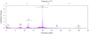 |
Fig. 4. Part of the Lomb-Scargle periodogram of KIC 3240967 computed from the Kepler long-cadence data in quarters 1–17 (Q1–Q17). The horizontal bars indicate the ranges of frequency groups A–E. Label X around 28 μHz indicates the position of non-significant peaks. |
This figure shows five frequency groups (A–E) that are located around 1, 8, 12, 20, and 40 μHz. We used the Aarhus University extraction of coherent oscillations (ECHO) pipeline (Antoci et al. 2019) to extract the frequencies of these groups. The list of frequencies is given in Table A.1.
Because of the highest amplitude, we may identify group D as Kelvin g-modes with m = 1 (cf. Paper I). The  diagram given in Fig. 5 demonstrates that the open red circles constructed from the frequencies in group D are generally aligned on a straight line. However, we also note that these points show small wiggles around the line, which might be interpreted as a signature of the sharp gradient in the chemical composition profiles just outside the convective core (cf. Paper I; Miglio et al. 2008; Kurtz et al. 2014; Saio et al. 2015). Li et al. (2019) pointed out that the same effect is likely to cause the dip in the P–ΔP diagram of Rossby modes of this star (see their Fig. 2). We note that most of the frequencies in group D do not have consecutive radial orders, and that Δin has to be fixed based on the diagram, as explained in Paper I and indicated by the cyan arrows in the diagram.
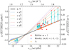 |
Fig. 5. Diagram of ν vs. |


We next identify group C with the second highest amplitude as Rossby modes with m = −1 and k = −2. This is confirmed by the fact that the open blue circles in Fig. 5, which are computed from the frequencies in group C, are roughly found on the same straight line as the open red circles (Kelvin g-modes).
While group B in Fig. 4 cannot be identified based on the  diagram, its frequency range relative to group C appears to be consistent with that of Rossby modes with m = −1 and k = −1 (Saio et al. 2018). In addition, this group contains some second-order combination frequencies between those in groups C and D (cf. Table A.1). A more detailed analysis is needed to identify modes of these frequencies. We note that even when a detected frequency can be expressed as a linear combination of other frequencies, it can still be an eigenfrequency. This is because it is possible that an eigenmode at the frequency is resonantly excited by the non-linear interaction to have a detectable amplitude. If this is the case, the combination frequency should be treated as a mode frequency in the asteroseismic analysis.
Three of the five frequencies in group E can be explained by the second-order combination frequencies. Their amplitudes of ∼0.1 mmag are larger by one order of magnitude than the products of the amplitudes of the parent frequencies with amplitudes of a few to several mmag. Although it is difficult to identify the remaining two frequencies, they are located at the expected position for Kelvin g-modes with m = 2 in the amplitude spectrum.
Many of the low-frequency peaks in group A might not be astrophysical because they are affected by the data analysis of the Kepler long-cadence data (e.g. Kurtz et al. 2014). Finally, non-significant peaks around 28 μHz, which are indicated by X in Fig. 4, might be those of Rossby modes with m = − 2 and k = − 2 (cf. Saio et al. 2018), or combination frequencies.
The results of the iterative linear least-squares fitting based on the frequencies in group D (Kelvin g-modes with m = 1) and/or group C (Rossby modes with m = − 1 and k = − 2) are provided in Table 2. We note that the points with the filled red circles in Fig. 5 were discarded in the fitting because they do not follow the expected behaviour of the Kelvin g-modes under the traditional approximation of rotation in the asymptotic regime. As discussed in Paper I, they might be affected by the avoided crossings or contamination of other types of modes. We can make qualitatively the same comments as in the case of the evolutionary model in Sect. 3: the analysis based on the Rossby modes alone requires as many as 11 iterations before convergence; this is because the spin parameter of the lowest-frequency mode is about 9, for which fi given by Eq. (13) deviates from its asymptotic value f0 (cf. Eq. (14)) by 18%; the converged values of νrot and P0 based on the Rossby modes alone and those on the Kelvin g-modes alone more or less agree with each other, although they are not strictly consistent within the given uncertainties; the simultaneous analysis of Kelvin g- and Rossby modes results in significant reduction of the uncertainties in and the correlation between νrot and P0. Our converged value of νrot based on both Kelvin g- and Rossby modes is completely consistent with Li et al. (2019), while that of P0 (4.25 × 10³ s) is larger than their estimate of 4.18 × 103 s by 2%. Although we find two peaks in the amplitude spectrum that have consistent frequencies with the estimated νrot and 2νrot within the uncertainties, they are not statistically significant.
Same as Table 1, but for KIC 3240967.
We note the amplitude structure of group C. Figure 6 shows the amplitude spectrum of group C, in which we observe two subgroups, C-I and C-II. Group C-I consists of modes below 12.5 μHz with consecutive radial orders. In this subgroup, the amplitude of the modes first increases as the frequency is higher. It becomes maximum at 12.3 μHz and decreases rapidly beyond this frequency. Group C-II is composed of four frequencies above 12.5 μHz, which have non-consecutive radial orders. Group C-II shows an isolated high peak of about 1 mmag at 12.85 μHz, which is indicated by an arrow in Fig. 6, while the peaks at the other frequencies are only about 0.2 mmag high. It might appear that the two subgroups originate from different types of modes because the amplitude distribution is clearly different between them. With the assumption of m = −1 and the rotation frequency of 14.9 μHz (cf. Table 2), we may estimate the spin parameters of the frequencies in group C-II to be 12.9 and above, which is consistent with those of Rossby modes with k = −3 (cf. Fig. 1). However, we reject this mode identification of group C-II because we fail to construct the  diagram with k = −3 that shows clear alignment of points on a straight line (or a smooth curve), in sharp contrast to Fig. 5. We thus regard all of the frequencies in group C as those of Rossby modes with m = −1 and k = −2. Still, we do not understand why the amplitude structure of these modes changes suddenly around 12.5 μHz. If the amplitude is determined by the mode visibility alone, the envelope of the amplitude in group C-I should extend as far as about the rotation frequency of 14.9 μHz (cf. Saio et al. 2018). The reason for the isolated peak at 12.85 μHz also needs to be explained. While we assume that the amplitude is controlled by the physical mechanism of mode excitation and damping, the problem needs to be discussed in more detail in a separate study. We finally note that the similar amplitude distribution of Rossby modes can also be found in other stars, including KIC 3448365 and KIC 9480469, the spectra of which are shown in Fig. A2 of Saio et al. (2018).
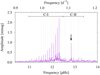 |
Fig. 6. Lomb-Scargle periodogram of KIC 3240967 around frequencies of group C. The vertical dotted lines indicate the extracted frequencies given in Table A.1. |
4.2. KIC 12066947
We analysed another γ Dor star, KIC 12066947, based on the  diagram. The amplitude spectrum of the star is shown in Fig. 7, and the extracted frequencies are listed in Table A.2. These frequencies were obtained by the method described in Antoci et al. (2019), and are found in five groups, which we refer to as groups U-0, U-1, A, B, and C in the order of frequency. Group B between 26 and 38 μHz consists of Kelvin g-modes with m = 1, and has been analysed in Christophe et al. (2018) and Paper I. On the other hand, group A between 19 and 25 μHz can be identified as Rossby modes with m = −1 and k = −2, as in Van Reeth et al. (2016). We note that in contrast to Christophe et al. (2018), we find the peaks between 56 and 69 μHz (group C) to be statistically significant. This is because after more detailed analyses, we discovered that using only data from the quarters Q10–Q17, hence removing Q0 and Q1 due to poorer quality, increases the number of extracted frequencies. We identify the frequencies in group C as Kelvin g-modes with m = 2. We also observe in Fig. 7 two more groups around 2 and 10 μHz, which are indicated by labels U-0 and U-1, respectively. The former could come from a combination frequencies or artefacts of data analysis, while the latter might originate from Rossby modes with m = −1 and k = −1. Figure 8 shows the
  diagram, and Table 3 provides the estimates of νrot and P0.
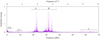 |
Fig. 7. Part of the Lomb-Scargle periodogram of KIC 12066947 computed from the Kepler long-cadence data in quarters 10–17 (Q10–Q17). The horizontal bars indicate the ranges of frequency groups. |
Same as Table 1, but for KIC 12066947.
We confirm the mode identification of group A based on the  diagram. The main difficulty comes from the non-consecutive radial orders: Δin > 1 for most cases. The problem can be solved using the results of Paper I based on Kelvin g-modes. By extending the best-fit line (of Paper I) on the diagram to the lower left side of the abscissa intercept, and drawing other lines with the common intercept and the slopes multiplied by
  ,
,  , …, we can verify whether each mode of group A is found on one of these lines. We can verify this when we assume m = −1 and k = −2, and obtain Δin for each point on the diagram, as indicated in Fig. 8. We can similarly verify the identification of group C as Kelvin g-modes with m = 2. We note that there are a few exceptional points with filled blue, red, and grey circles in Fig. 8. Because these points have too large Δin to be identified reliably or do not align on the straight line that the other points do, we excluded them from the fitting process to estimate νrot and P0.
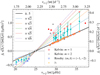 |
Fig. 8. Diagram of ν vs. |

When we have found Δin, we can analyse groups A, B, and C separately. The results based on group A alone (Rossby modes with m = −1 and k = −2), group B (Kelvin g-modes with m = 1), and group C (Kelvin g-modes with m = 2) are given in rows 3–5, 6–8, and 9–11 of Table 3, respectively. The converged values of the parameters νrot and P0 are consistent within the formal uncertainties in the three cases. Comparing the results for groups A and B, we find that the uncertainties in νrot are similar (∼0.3%), and that the error in P0 is larger for group A (6%) than for group B (2%). On the other hand, the uncertainties in νrot and P0 for group C are larger by about an order of magnitude than those for group B.
The three types of modes can be used simultaneously to obtain the results in rows 12–14 of Table 3. The uncertainties in the two parameters are smaller by a few factors than in the separate analysis of group B. These estimates are completely consistent with those of Li et al. (2019), who considered only the two types, Rossby modes (with m = −1 and k = −2) and Kelvin g-modes with m = 1. As in the case of Sect. 3.2, the correlation coefficient between the estimated νrot and P0 is significantly reduced to 0.56 because different types of modes are used. In addition, the outputs of the first iteration, νrot = 24.88 μHz and P0 = 4.07 × 10³ s, are different from the converged values of νrot = 24.98 ± 0.02 μHz and P0 = (4.20±0.03) × 103 s, by only 0.4% and 3%, respectively. We note that there is a non-significant peak in the Lomb-Scargle periodogram at the frequency consistent with νrot = 24.98 ± 0.02 μHz.
5. Discussion and conclusion
We have extended the method of the  diagram to take not only Kelvin g-modes, but also Rossby modes with k ≤ −2 into account in order to diagnose the internal structure of γ Dor stars from their oscillations. Kelvin and Rossby modes are the most and second most frequently detected modes in γ Dor stars, respectively. The majority of the observed modes are identified as either one or the other of these modes (e.g. Li et al. 2020). The (average) rotation frequency νrot and the characteristic period of gravity-mode oscillations P0 can be estimated by the iterative linear fitting based on the diagram. The extension was made straightforwardly by noting that as in the case of Kelvin g-modes, the frequencies of Rossby modes with k ≤ −2 tend to be independent of νrot in the co-rotating frame for large νrot. Rossby modes are located in the region of negative ordinates and lower frequencies than Kelvin g-modes in the diagram. The rotation frequency νrot is found between the frequency distributions of the two modes. The estimates of νrot and P0 are significantly improved when Kelvin and Rossby modes are used simultaneously in the following two points: (1) reduction of the uncertainties and (2) a lower (anti-)correlation between the estimates. These were confirmed first with a theoretical model in Sect. 3 and then based on two Kepler stars, KIC 3240967 and KIC 12066947, in Sect. 4. According to Fig. 13 of Li et al. (2020), the estimated rotation frequency of 14.887 ± 0.008 μHz (1.2862 ± 0.0007 d−1) of the former is typical for γ Dor stars, while that of the latter of 24.98 ± 0.02 μHz (2.158 ± 0.002 d−1) is close to the upper end of the distribution.
Eigenmodes of low-frequency oscillations in rotating stars can generally be classified in the traditional approximation of rotation. Each type of modes corresponds to a sequence of eigenvalues of the Laplace tidal equation, λ, which is a function of the spin parameter s (cf. Fig. 1). The behaviour of Kelvin g-modes and Rossby modes with k ≤ −2 is different from the other types of modes because only these two types have finite λ as s becomes large, while λ of the other types diverges quadratically (λ ∝ s2) (e.g. Townsend 2003). Because large λ means short horizontal wavelengths, which lead to significant geometrical cancellation, these types of modes are quite difficult to detect in rapid rotators. The convergence of λ to finite values is a key point for the method of the  diagram because the (quasi-)linear relation of Eq. (10) is derived from this property. It is just fortunate that the problem can be reduced to a linear one only for the modes that are easy to observe.
Although Kelvin and Rossby modes are different in their physical characters and in the observed frequency ranges, they provide almost the same information (particularly about the two structural parameters νrot and P0) in so far as the degree of differential rotation is weak. This is because their frequencies can both be quite accurately explained by Eq. (1) in the traditional approximation of rotation. They differ only in the value of λ. The inner turning points of their propagation cavity are essentially fixed by the outer edge of the convective core, while the outer turning points can weakly depend on the frequency. However, the effect on the integrals in Eqs. (2) and (3) is limited because the dominant contribution comes from the layers just outside the convective core where the Brunt–Väisälä frequency has a high peak. Because the two types of modes give almost the same average of the rotation profile, the possibility of weak differential rotation (in the radial direction) cannot be rejected even though the estimates of νrot between them in Sect. 4 are consistent with each other. The latitudinal differential rotation can also be studied using the fact that Kelvin and Rossby modes have large amplitudes near the equator and in the mid-latitude region, respectively. More detailed analyses are clearly needed.
While the frequencies of γ Dor stars can mostly be interpreted in the traditional approximation of rotation, the uncertainties in the observed data taken by Kepler are so small that in the next step, we need to correct the approximation to fully understand the fine structure of the frequency spectrum (cf. Sect. 3). Another direction of future study is to apply the method to rapidly rotating hybrid pulsators of γ Dor and δ Sct type (e.g. Grigahcène et al. 2010). Estimates of νrot and P0 from the low-frequency modes will be helpful to understand the spectrum of the high-frequency modes, which is known to be very complicated (e.g. Dziembowski 1990).
Acknowledgments
We thank NASA and the Kepler team for their revolutionary data. M.T. is partially supported by JSPS KAKENHI Grant Number JP18K03695. S.J.A.J.S. has received funding from the European Research Council (ERC) under the European Union’s Horizon 2020 research and innovation programme (Grant agreement No 833925, project STAREX). This work was supported by a research grant (00028173) from VILLUM FONDEN. Funding for the Stellar Astrophysics Centre is provided by The Danish National Research Foundation (Grant agreement no.: DNRF106).
References
- Antoci, V., Cunha, M. S., Bowman, D. M., et al. 2019, MNRAS, 490, 4040 [NASA ADS] [CrossRef] [Google Scholar]
- Baglin, A., Auvergne, M., Boisnard, L., et al. 2006, in 36th COSPAR Scientific Assembly, COSPAR Meeting, 36 [Google Scholar]
- Ballot, J., Lignières, F., Prat, V., Reese, D. R., & Rieutord, M. 2012, in Progress in Solar/Stellar Physics with Helio- and Asteroseismology, eds. H. Shibahashi, M. Takata, & A. E. Lynas-Gray, ASP Conf. Ser., 462, 389 [NASA ADS] [Google Scholar]
- Beck, P. G., Bedding, T. R., Mosser, B., et al. 2011, Science, 332, 205 [NASA ADS] [CrossRef] [PubMed] [Google Scholar]
- Beck, P. G., Montalban, J., Kallinger, T., et al. 2012, Nature, 481, 55 [NASA ADS] [CrossRef] [Google Scholar]
- Bedding, T. R., Huber, D., Stello, D., et al. 2010, ApJ, 713, L176 [NASA ADS] [CrossRef] [Google Scholar]
- Bedding, T. R., Mosser, B., Huber, D., et al. 2011, Nature, 471, 608 [NASA ADS] [CrossRef] [PubMed] [Google Scholar]
- Borucki, W. J., Koch, D., Basri, G., et al. 2010, Science, 327, 977 [NASA ADS] [CrossRef] [PubMed] [Google Scholar]
- Chaplin, W. J., & Miglio, A. 2013, ARA&A, 51, 353 [NASA ADS] [CrossRef] [Google Scholar]
- Christophe, S., Ballot, J., Ouazzani, R.-M., Antoci, V., & Salmon, S. J. A. J. 2018, A&A, 618, A47 [NASA ADS] [CrossRef] [EDP Sciences] [Google Scholar]
- Deheuvels, S., Garcia, R. A., Chaplin, W. J., et al. 2012, ApJ, 756, 19 [NASA ADS] [CrossRef] [Google Scholar]
- Deheuvels, S., Doğan, G., Goupil, M. J., et al. 2014, A&A, 564, A27 [NASA ADS] [CrossRef] [EDP Sciences] [Google Scholar]
- Dziembowski, W. 1990, in Toward Seismology of δ Scuti Stars, eds. Y. Osaki, & H. Shibahashi, 367, 359 [Google Scholar]
- Eckart, C. 1960, Hydrodynamics of Oceans and Atmospheres (New York: Pergamon Press) [Google Scholar]
- Gill, A. 1982, Atmosphere-ocean Dynamics (New York: Academic Press) [Google Scholar]
- Gough, D. 1985, Sol. Phys., 100, 65 [NASA ADS] [CrossRef] [Google Scholar]
- Grigahcène, A., Antoci, V., Balona, L., et al. 2010, ApJ, 713, L192 [NASA ADS] [CrossRef] [Google Scholar]
- Kurtz, D. W., Saio, H., Takata, M., et al. 2014, MNRAS, 444, 102 [NASA ADS] [CrossRef] [Google Scholar]
- Lee, U., & Saio, H. 1997, ApJ, 491, 839 [NASA ADS] [CrossRef] [Google Scholar]
- Li, G., Van Reeth, T., Bedding, T. R., Murphy, S. J., & Antoci, V. 2019, MNRAS, 487, 782 [Google Scholar]
- Li, G., Van Reeth, T., Bedding, T. R., et al. 2020, MNRAS, 491, 3586 [NASA ADS] [CrossRef] [Google Scholar]
- Miglio, A., Montalbán, J., Noels, A., & Eggenberger, P. 2008, MNRAS, 386, 1487 [NASA ADS] [CrossRef] [Google Scholar]
- Mosser, B., Barban, C., Montalbán, J., et al. 2011, A&A, 532, A86 [NASA ADS] [CrossRef] [EDP Sciences] [Google Scholar]
- Osaki, Y. 1975, PASJ, 27, 237 [NASA ADS] [Google Scholar]
- Ouazzani, R.-M., Dupret, M.-A., & Reese, D. R. 2012, A&A, 547, A75 [NASA ADS] [CrossRef] [EDP Sciences] [Google Scholar]
- Ouazzani, R.-M., Roxburgh, I. W., & Dupret, M.-A. 2015, A&A, 579, A116 [NASA ADS] [CrossRef] [EDP Sciences] [Google Scholar]
- Ouazzani, R.-M., Salmon, S. J. A. J., Antoci, V., et al. 2017, MNRAS, 465, 2294 [NASA ADS] [CrossRef] [Google Scholar]
- Papaloizou, J., & Pringle, J. E. 1978, MNRAS, 182, 423 [NASA ADS] [CrossRef] [Google Scholar]
- Ricker, G. R., Winn, J. N., Vanderspek, R., et al. 2014, in Transiting Exoplanet Survey Satellite (TESS), SPIE Conf. Ser., 9143, 914320 [Google Scholar]
- Rossby, C. G. 1939, J. Mar. Res., 2, 38 [NASA ADS] [CrossRef] [Google Scholar]
- Saio, H. 2018, ArXiv e-prints [arXiv:1812.01253] [Google Scholar]
- Saio, H., Kurtz, D. W., Takata, M., et al. 2015, MNRAS, 447, 3264 [Google Scholar]
- Saio, H., Kurtz, D. W., Murphy, S. J., Antoci, V. L., & Lee, U. 2018, MNRAS, 474, 2774 [Google Scholar]
- Schmid, V. S., Tkachenko, A., Aerts, C., et al. 2015, A&A, 584, A35 [NASA ADS] [CrossRef] [EDP Sciences] [Google Scholar]
- Takata, M., Ouazzani, R.-M., Saio, H., et al. 2020, A&A, 635, A106 [Google Scholar]
- Thomson, W. 1880, Proc. R. Soc. Edinburgh, 10, 92 [CrossRef] [Google Scholar]
- Townsend, R. H. D. 2003, MNRAS, 340, 1020 [Google Scholar]
- Van Reeth, T., Tkachenko, A., Aerts, C., et al. 2015, ApJS, 218, 27 [Google Scholar]
- Van Reeth, T., Tkachenko, A., & Aerts, C. 2016, A&A, 593, A120 [NASA ADS] [CrossRef] [EDP Sciences] [Google Scholar]
Appendix A: Additional tables
Frequency list of KIC 3240967.
Frequency list of KIC 12066947.
All Tables
Estimates of νrot and P0 for the evolutionary model of a γ Dor star (Model A of Christophe et al. 2018).
All Figures
|
Fig. 1. Profiles of |
| In the text | |
|
Fig. 2. Diagram of ν vs. |
| In the text | |
|
Fig. 3. Same as Fig. 2, but based on both Kelvin and Rossby modes, which are denoted by open red and blue circles, respectively. Small open orange circles represent |
| In the text | |
|
Fig. 4. Part of the Lomb-Scargle periodogram of KIC 3240967 computed from the Kepler long-cadence data in quarters 1–17 (Q1–Q17). The horizontal bars indicate the ranges of frequency groups A–E. Label X around 28 μHz indicates the position of non-significant peaks. |
| In the text | |
|
Fig. 5. Diagram of ν vs. |
| In the text | |
|
Fig. 6. Lomb-Scargle periodogram of KIC 3240967 around frequencies of group C. The vertical dotted lines indicate the extracted frequencies given in Table A.1. |
| In the text | |
|
Fig. 7. Part of the Lomb-Scargle periodogram of KIC 12066947 computed from the Kepler long-cadence data in quarters 10–17 (Q10–Q17). The horizontal bars indicate the ranges of frequency groups. |
| In the text | |
|
Fig. 8. Diagram of ν vs. |
| In the text | |
Current usage metrics show cumulative count of Article Views (full-text article views including HTML views, PDF and ePub downloads, according to the available data) and Abstracts Views on Vision4Press platform.
Data correspond to usage on the plateform after 2015. The current usage metrics is available 48-96 hours after online publication and is updated daily on week days.
Initial download of the metrics may take a while.