| Issue |
A&A
Volume 644, December 2020
|
|
|---|---|---|
| Article Number | A105 | |
| Number of page(s) | 17 | |
| Section | Astrophysical processes | |
| DOI | https://doi.org/10.1051/0004-6361/202037724 | |
| Published online | 08 December 2020 | |
Constraining the accretion flow density profile near Sgr A* using the L′-band emission of the S2 star
1
I. Physikalisches Institut der Universität zu Köln, Zülpicher Strasse 77, 50937 Köln, Germany
e-mail: This email address is being protected from spambots. You need JavaScript enabled to view it.
2
Max-Planck-Institut für Radioastronomie (MPIfR), Auf dem Hügel 69, 53121 Bonn, Germany
3
Centre for Theoretical Physics, Polish Academy of Sciences, Al. Lotnikow 32/46, 02-668 Warsaw, Poland
4
Institut für Astro- und Teilchenphysik, Universität Innsbruck, Technikerstrasse 25/8, 6929 Innsbruck, Austria
Received:
13
February
2020
Accepted:
27
September
2020
Abstract
Context. The density of the ambient medium around a supermassive black hole (SMBH) and the way it varies with distance plays an important role in our understanding of the inflow-outflow mechanisms in the Galactic centre (GC). This dependence is often fitted by spherical power-law profiles based on observations in the X-ray, infrared (IR), submillimetre (submm), and radio domains.
Aims. Nevertheless, the density profile is poorly constrained at the intermediate scales of 1000 Schwarzschild radii (Rs). Here we independently constrain the spherical density profile using the stellar bow shock of the star S2 which orbits the SMBH at the GC with the pericentre distance of 14.4 mas (∼1500 Rs).
Methods. Assuming an elliptical orbit, we apply celestial mechanics and the theory of bow shocks that are at ram pressure equilibrium. We analyse the measured IR flux density and magnitudes of S2 in the L′-band (3.8 micron) obtained over seven epochs in the years between 2004–2018. We put an upper limit on the emission from S2’s associated putative bow shock and constrain the density profile of the ambient medium.
Results. We detect no significant change in S2 flux density until the recent periapse in May 2018. The intrinsic flux variability of S2 is at the level of 2–3%. Based on the dust-extinction model, the upper limit on the number density at the S2 periapse is ∼1.87 × 109 cm−3, which yields a density slope of at most 3.20. Using the synchrotron bow-shock emission, we obtain the ambient density of ≲1.01 × 105 cm−3 and a slope of ≲1.47. These values are consistent with a wide variety of media from hot accretion flows to potentially colder and denser media comparable in properties to broad-line-region clouds. However, a standard thin disc can be excluded at the distance of S2’s pericentre.
Conclusions. With the current photometry sensitivity of 0.01 mag, we are not able to make stringent constraints on the density of the ambient medium in the GC using S2-star observations. We can distinguish between hot accretion flows and thin, cold discs, where the latter can be excluded at the scale of the S2 periapse. Future observations of stars in the S cluster using instruments such as Mid-IR Extremely Large Telescope Imager and Spectrograph at Extremely Large Telescope with the photometric sensitivity of as much as 10−3 mag will allow the GC medium to be probed at intermediate scales at densities as low as ∼700 cm−3 in case of non-thermal bow-shock emission. The new instrumentation, in combination with discoveries of stars with smaller pericentre distances, will help to independently constrain the density profile around Sagittarius A* (Sgr A*).
Key words: infrared: stars / black hole physics / Galaxy: center
© S. Elaheh Hosseini et al. 2020
 Open Access article, published by EDP Sciences, under the terms of the Creative Commons Attribution License (https://creativecommons.org/licenses/by/4.0), which permits unrestricted use, distribution, and reproduction in any medium, provided the original work is properly cited.
Open Access funding provided by Max Planck Society.
1. Introduction
The Galactic centre (GC) is a unique astrophysical setting where one can study the dynamical effects in one of the densest stellar clusters (Alexander 2005; Merritt 2013; Schödel et al. 2014) and the mutual interaction of stars, gaseous-dusty structures, the magnetic field, and the supermassive black hole (SMBH; Genzel et al. 2010; Eckart et al. 2017). The dynamical centre traced by orbiting stars coincides with the non-thermal compact and variable radio source Sagittarius A* (Sgr A*) within 0.03″ (Menten et al. 1997). Because of its well-constrained mass of MBH = (4.15 ± 0.13 ± 0.57)×106 M⊙ (Parsa et al. 2017) based mainly on monitoring of fast-moving S stars (see also Schödel et al. 2002; Ghez et al. 2008; Gillessen et al. 2009, 2017; Boehle et al. 2016), Sgr A* is associated with the SMBH, leaving only a little space for alternative scenarios of its compact nature (Eckart et al. 2017). Given its distance of 8.1 kpc (Eisenhauer et al. 2003; Reid et al. 2003; Gravity Collaboration 2019), it is the nearest SMBH, which allows us to perform high-precision astrometric and interferometric observations of Sgr A* and its immediate surroundings. In recent years, this provided an opportunity to confirm general relativistic predictions by measuring the gravitational redshift (Gravity Collaboration 2018a; Do et al. 2019a) as well as the Schwarzschild precession (Gravity Collaboration 2020) by monitoring the bright S2 star (also referred to as S0-2) that orbits Sgr A* with a period of 16.2 years.
Sgr A* belongs to extremely low-luminous sources, with its bolometric luminosity that is eight to nine orders of magnitude below its Eddington limit (Narayan et al. 1998; Yuan & Narayan 2014). Its broadband spectral energy distribution is best described by a class of radiatively inefficient accretion flows (RIAFs; Yuan et al. 2003). In order to better comprehend its low-luminous, diluted accretion flow, it is of prime importance to constrain its density at large, intermediate, and eventually small spatial scales. This has been done by analysing the radiative properties of its surroundings. At larger scales, the analysis of the X-ray bremsstrahlung emissivity profile of 1.3 keV plasma in the central hot bubble yielded a number density of  (with ηf being the filling factor), close to the Bondi radius (Baganoff et al. 2003; Wang et al. 2013), which lies at rB ≈ 4″(Ta/107 K)−1 ≈ 0.16 pc given the plasma temperature Ta (Wang et al. 2013). Density constraints at the scale of 10–100 Schwarzschild radii (hereafter denoted rs) were obtained by analysing the polarised millimetre (mm) and submillimetre (submm) emission, which implies non-thermal self-absorbed synchrotron radiation in the mm domain that becomes optically thin at submm wavelengths (Aitken et al. 2000; Agol 2000; Bower et al. 2003). Marrone et al. (2006, 2007) detected the Faraday rotation of the polarised submm emission based on which they constrain the accretion-rate of Sgr A* to Ṁ ∼ 2 × 10⁻⁹ − 2 × 10⁻⁷ M⊙ yr−1, which corresponds to the maximum number density of
  close to the event horizon. Generally, the hot accretion flow in the GC is described by a power-law density profile n ∝ r−γ, where the power-law slope is typically inferred to be γ ∼ 0.5−1.0 (Wang et al. 2013) in agreement with the RIAF-type flows. Spherical Bondi-type flow with γ ∼ 3/2 is also consistent with the X-ray surface brightness profile up to 3″ from Sgr A* (Różańska et al. 2015). Hence, the number densities of the ambient flow and the corresponding slopes are still quite uncertain, especially at intermediate spatial scales where the fast-moving S stars are located. This uncertainty was further enhanced by the possible detection of a cooler (∼104 K) and a denser disc with a number density of ∼105 − 106 cm−3 at the radius of ∼0.004 pc, which is comparable to the semi-major axis of the bright S2 star (Murchikova et al. 2019). However, the detection by Murchikova et al. (2019) is questionable, especially the association of the recombination double-peak line of H30α at 1.3 mm with the gaseous material at milliparsec spatial scales; it is especially controversial given that near-infrared (NIR) line maps, for example of the recombination Brγ line that can trace ionised material of 104 K, do not seem to imply any existence of such a compact disc-like structure. On the other hand, there are indications of denser material traced by the Brγ line (Peißker et al. 2020a) and the blueshifted H30α line (Royster et al. 2019) at larger spatial scales closer to the Bondi radius, which the study of Murchikova et al. (2019) could be associated with. This underlines the need for better and independent constraints on the accretion-flow density at the intermediate range of radii.
The fast-moving stars of the S cluster could in principle be used to constrain the accretion flow density at intermediate scales. As fast-moving probes, these stars drive shocks into the ambient medium and provide radiative energy that can temporarily affect the radiative properties of the accretion flow as well as form localised density and extinction enhancements. Any detected flares linked to an orbiting star would thus provide a way to infer density and other properties of the intercepted ambient medium. Quataert & Loeb (2005) analysed the possibility that the stellar wind shocks in the central arcsecond could contribute to the ambient TeV and non-thermal broadband emission. It was predicted that the interaction of the fast-moving B-type S2 star with the ambient hot accretion flow is expected to form a bow shock, which should result in a month-long thermal X-ray bremsstrahlung flare with the peak luminosity of LX = 4 × 1033 erg s−1 (Giannios & Sironi 2013; Christie et al. 2016). The contribution to the emerging X-ray flux is also expected to come from UV and optical photons of S2 that are Compton-upscattered by electrons of the inner hot RIAF (Nayakshin 2005). According to these models, the S2 bow-shock X-ray luminosity is in principle comparable to the quiescent X-ray emission of Sgr A* and hence could be detected with the current X-ray instruments. The non-detection of any significant X-ray flare around the pericentre crossings of S2 star in 2002 and 2018 is consistent with a diluted hot RIAF flow in the central arcsecond (Yuan et al. 2003). The low X-ray flux from the bow shock is also in agreement with numerical 3D adaptive-mesh refinement simulations of the motion of S2 through the RIAF (Schartmann et al. 2018).
The detection and the monitoring of the dusty G2 source or the Dusty S-cluster Object (DSO; Gillessen et al. 2012; Eckart et al. 2013; Witzel et al. 2014; Valencia-S et al. 2015; Peißker et al. 2020b; Ciurlo et al. 2020) triggered an effort to predict and observe its potential interaction with the ambient environment. Narayan et al. (2012) predicted the radio synchrotron emission from the DSO bow shock to be comparable to the quiescent radio emission of Sgr A*. In theory, electrons in the ambient accretion flow are expected to be accelerated in the bow-shock region. The main sources of uncertainty are the bow-shock size, which depends on the stellar-wind characteristics and the ambient density, and the magnetic field strength that is enhanced in the bow shock. For the more realistic estimates of the DSO/G2 bow-shock size, assuming the low-mass star model, the radio synchrotron emission was calculated to be well below the radio emission of Sgr A*, and therefore no detectable flare was expected (Crumley & Kumar 2013; Zajaček et al. 2016). This was observationally confirmed by the non-detection of any enhanced radio or mm emission by Bower et al. (2015) and Borkar et al. (2016), who constrain the DSO/G2 cross-section to < 2 × 1029 cm2.
The bow-shock synchrotron emission can be generalised to the S stars, predicting their broad-band synchrotron spectrum with the peak close to 1 GHz and associated monochromatic light-curves (Ginsburg et al. 2016). Ginsburg et al. (2016) estimated that the synchrotron emission from S-star bow shocks can be comparable to the Sgr A* radio (10 GHz) and IR flux densities (1014 GHz) for rather extreme combinations of the wind mass-loss rate and its terminal velocity – (ṁw,vw) = (10−5 M⊙ yr−1, 103 km s−1) and (ṁw,vw) = (10−6 M⊙ yr−1, 4 × 10³ km s−1). These values deviate from those inferred for S2 (Martins et al. 2008; Habibi et al. 2017): (ṁw,vw) = (<3 × 10⁻⁷ M⊙ yr−1, 103 km s−1). For these observationally inferred values, the S star non-thermal flux densities are below those of Sgr A*. Another, independent way to constrain the density of the ambient medium is the detection of deviation from the Keplerian ellipse due to hydrodynamic drag force. Gillessen et al. (2019) claimed the detection of a significant deviation for the DSO/G2 object due to the drag force, from which they inferred a density of 4 × 103 cm−3 at the DSO/G2 pericentre close to 1000 rs.
Here we report NIR L′-band emission from one of the brightest members of the S cluster, star S2. Close to its first observed pericentre passage in 2002, Clénet et al. (2004) reported a brightening of S2 in L′-band, which could be associated with its interaction with the ambient medium at the scale of 1500 Schwarzschild radii1. Based on our reanalysis of the 2002 epoch and an additional seven epochs, including close to the subsequent pericentre passage in 2018, we can exclude any significant brightening related to the pericentre passage of S2 in L′-band. The intrinsic fractional variability of the S2 light curve is only ∼2.5%. Using the model of the thermal dust emission in the shocked ambient medium, we place an upper limit on the ambient density of ≲109 cm−3, which can accommodate a wide variety of ambient media at the S2 pericentre distance of 1500 Schwarzschild radii, except for a standard thin cold disc. The bow-shock synchrotron model gives a tighter upper limit of ∼105 cm−3. An improved photometric sensitivity of the next-generation of instruments, in particular Mid-IR Extremely Large Telescope Imager and Spectrograph (METIS) at Extremely Large Telescope (ELT), will help to further constrain the density at intermediate scales.
The current paper is structured as follows. Section 2 describes the observations and data-reduction methods used for this work. We then briefly discuss the photometry and its results for S2 in Sects. 2.1 and 2.2, respectively. In Sect. 3 we constrain the slope and density of the ambient accretion flow using S2 star observations in L′ band. Section 3.1 is dedicated to the exploration of the extinction caused by the ambient gas and dust inside the Bondi radius. In Sect. 3.2, the upper limit of the ambient density is inferred based on the thermal bow-shock emission. In Sect. 3.3, we then constrain the ambient density based on the non-thermal bow-shock emission. We discuss the obtained density values in the broader context of the accretion flows and the GC gaseous-dusty structures in Sect. 4. Finally, in Sect. 5 we summarise the main results.
2. Observations and data reduction
Observations of the GC in the NIR were carried out with the European Southern Observatory (ESO) Very Large Telescope (VLT) Unit 1 (UT1)-YEPUN on Paranal, Chile. The data were obtained from the IR camera Coude NIR Camera (CONICA) and the Nasmyth Adaptive Optics System (NAOS) adaptive optics (AO) module, known as NACO. The central parsec of the GC has been frequently observed with the VLT in the L′-band (3.8 μm, 0.0271″ pixel−1).
In Table 1, we summarise the obtained data that are analysed in this study. The total time-coverage of the data set is from 2004.317 until 2018.307. The only applied criterion on the epoch selection is the imaging quality, because a large number of the available data sets in the archive were observed during poor atmospheric conditions, in particular bad and fast seeing. We used the standard data-reduction process that consists of the sky subtraction, flat-fielding, and bad pixel correction for all imaging data and combined them via a shift-add algorithm to obtain a final array size of 28″ × 28″ for all epochs.
L′-band flux and magnitude of S2 and S65 for seven epochs over a 15-year interval from 2004.317 to 2018.307.
The first observed periapse of S2 occurred in 2002. The spatial resolution of NACO at 3.8 μm is 0.096″, while the distance between Sgr A* and S2 in 2002 is approximately 0.040″. Therefore, it is impossible to obtain the emission of S2 from the images completely separated from Sgr A* emission. Furthermore, we know that Sgr A* is flaring in the observation which is done in 2002 (Genzel et al. 2003), and in 2002 and 2003 the NIR-excess extended source denoted G1 is sufficiently close to the S2-Sgr A* system that it cannot be disentangled from the Sgr A*-S2 system (Clénet et al. 2004; Witzel et al. 2017).
We show the superposition of S2 and G1 in Fig. 1, where we plot the projected orbits of S2, G1, and DSO/G2. Immediately before the pericentre passage around 2002, the mutual separation between S2 and G1 was less than 0.1 arcsec; see Fig. 1 (left panel). The G1 cloud is currently going to larger distances from Sgr A* (more than 0.2 arcsec, see Fig. 1, right panel), and therefore potential changes of the brightness of S2 after 2002 pericentre passage would be due to other effects, most likely due to bow-shock emission, which we analyse in this contribution. Hence, to prevent further uncertainties in our analysis, we excluded the first observed periapse of S2.
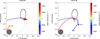 |
Fig. 1. S2 star and known dusty objects close to its orbit. Left panel: position of S2 and the dusty source G1 close to the pericentre of S2 around 2002. We also show the orbit of the DSO (Dusty S-cluster Object, also known as G2). The points of the sources represent colour-coded radial velocities according to the axis on the right. The grey circle in the bottom left corner represents the diffraction limited FWHM of 98 mas corresponding to NACO L′-band. Right panel: position of S2 and dusty source G1 at the pericentre passage of S2 at 2018.38. The orbital parameters were adopted from Gravity Collaboration (2018a) (S2 star), Valencia-S et al. (2015) (DSO source), and Witzel et al. (2017) (G1 source). |
2.1. Photometry
Flux densities of S2 and calibrators were determined via aperture photometry using a circular aperture of 82 mas in L′-band. Dereddened fluxes were computed with the extinction of AL = 1.09 ± 0.13 (Fritz et al. 2011) and a zero magnitude value of F0(L) = 249 Jy.
The magnitude calibration is done by considering S26, S30, and S35 as calibrators using their known brightness from Gillessen et al. (2009). These S-stars are chosen because they are sufficiently isolated over the epochs of our study. In Fig. 2, we show the surroundings of S2 within about ±1″ on 9 May 2013.
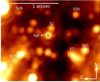 |
Fig. 2. NACO L′-band mosaic of the GC in 2013.356. North is up and east is to the left. The identification of three stars (S26, S30 and S35) as photometric calibrators is depicted in particular. The black cross shows the IR counterpart of Sgr A*. In order to check any variability in the flux of S2, we used S65 as a reference star. |
In general, the grainy background at the centre of our Galaxy is variable due to the proper motion of the stars (Sabha et al. 2012). Therefore, to correct for background brightness, we used five apertures with the same size as our photometric apertures close enough to the calibrators and S2 to get an appropriate representative of the existing background. Because of the high-velocity S-stars, the background is highly variable, and therefore background apertures are not located at the same position for all the epochs considered in this study.
2.2. Photometry results
S2 is an early B-type dwarf of spectral type B0–B2.5 V with a stellar wind that has an estimated velocity of vw ∼ 1000 km s−1 and a mass-loss rate of ṁw ≲ 3 × 10⁻⁷ M⊙ yr−1 (Martins et al. 2008). We did the aperture photometry with local background subtraction for seven selected epochs from 2004 to 2018. S65 flux and magnitude were also studied in order to use this object as a test star to reveal any meaningful changes in S2 flux or magnitude.
The photometry results are presented in Table 1. As shown in Fig. 3, there is essentially no change detected in the measured flux density of S2 within the uncertainties over the seven epochs. The total coverage is 15 years, which is close to the S2 orbital period around Sgr A*, including epochs close to the pericentre passages of S2. The light curve has a mean value of the flux density of  , with a difference between maximum and minimum values of 0.90 mJy. In terms of the L′-band magnitude, the mean magnitude of S2 in the L′-band is 11.12 ± 0.04. The intrinsic variability of S2 is characterised by a normalised excess variance (Nandra et al. 1997),
![Mathematical equation: $$ \begin{aligned} \sigma _{\rm rms}^2=\frac{1}{N\overline{f}^2}\sum _{i=1}^{N}[(f_i-\overline{f})^2-\sigma _i^2], \end{aligned} $$](/articles/aa/full_html/2020/12/aa37724-20/aa37724-20-eq5.gif) (1)
(1)
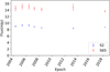 |
Fig. 3. Light curve of S2 and S65 in L′-band over seven observational epochs. |
where fi are individual flux measurements,  is the mean flux density, and σi are individual measurement errors. We obtain the value of the fractional variability
  in terms of the flux density and Mvar = 0.22% in terms of the magnitude. For the control star S65, we obtain Fvar = 4.53%, which is almost a factor of two larger than S2. These values are fully consistent with no intrinsic changes in the L′-band flux density of S2 within measurement uncertainties. For completeness, the mean, the maximum difference, and the fractional variability Fvar are listed in Table 1 for both S2 and S65.
In order to study the S2 flux and magnitude closely during its periapse in May 2018 at around 1500 Rs distance from Sgr A*, we performed the aperture photometry on all single exposures from the observation on 2018.307, on the position of S2 and the IR counterpart of radio source Sgr A*. The physical separation of S2 and Sgr A* was only 1.38 mpc, corresponding to 34.6 mas, while the angular resolution is 99.5 mas in L′-band. The photometry results are shown in Fig. 4. As can be seen, there is no sudden increase in the received flux from the position, and therefore Sgr A* is in its quiescent state in L′-band over the observation 2018.307. In addition to the non-detection of any flare from the IR counterpart of Sgr A*, no apparent increase in the S2 flux was observed within the measurement uncertainties.
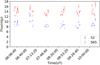 |
Fig. 4. Light curve at the position of S2 and the IR counterpart of Sgr A* and our reference star, S65, in 2018.307 in L′-band. The light curve shows that the IR counterpart of Sgr A* is in quiescence during our observation, and therefore the light curve belongs to S2. |
For the 2002.663 epoch, we measure 17.41 ± 1.18 mJy at the –at that time– combined position of S2, G1, and L′-band counterpart of Sgr A*. Taking into account S2’s mean stellar flux density of 8.88 ± 0.33 mJy (dreddened with AL = 1.09) and the G1 L′-band flux density of ∼2.58 ± 1.40 mJy close to the 2002 epoch (Witzel et al. 2017), the flux of Sgr A* ends up being around 6.03 ± 0.52 mJy. Schödel et al. (2011) obtains the mean flux of Sgr A* in the L′-band as 4.33 ± 0.18 mJy, which leads us to 1.70 mJy surplus in the measured flux density. However, due to the lack of a longer (at least days) light-curve time coverage during the S2 periapse passage of the variable source black hole counterpart SgrA* in 2002, it is not possible to determine whether this flux density excess is due to a Sgr A* flare or the S2 stellar bow-shock effect. However, since during the subsequent pericentre passage in 2018 the flux density of S2 is within the uncertainty comparable to its mean value (see Table 1), the excess can be attributed to the Sgr A* flare, unless the accretion flow density changes dramatically by several orders of magnitude from one periapse to another. The flux excess of 1.70 mJy that corresponds to the magnitude change of ∼0.19 mag would require the pericentre number density of ∼4.2 × 1010 cm−3 according to the dust-extinction model we present in Sect. 3.2. Considering the synchrotron bow-shock emission (see Sect 3.3), the required density at the pericentre is smaller, na ∼ 2.1 × 105 cm−3, but still larger by two orders of magnitude than expected for the RIAF density profile with γ ≈ 1, na ∼ 7.2 × 103 cm−3. Such a large density present only for epoch 2002 is unlikely. The excess flux of 1.70 mJy can therefore be attributed to the L′-band flare of Sgr A*. In the L′-band, Sgr A* is permanently variable (Schödel et al. 2011) with the flux densities in the range between 1 mJy and 10 mJy (Ghez et al. 2005; Eckart et al. 2008; Dodds-Eden et al. 2009).
3. Constraining the slope and density of the ambient accretion flow using S2’s L′-band emission
In this section, we develop a simple method for inferring the density slope and the maximum density at the pericentre of a wind-blowing star using the observed light curve and an analytical dust extinction model. This method is suitable for stars with an unresolved bow shock. For a fully resolved bow shock at least two positions of a star along an elliptical orbit, one can infer the density slope from the bow-shock size ratio and an orbital eccentricity; see Appendix B for more details. Furthermore, we also consider the non-thermal bow-shock emission as an independent way of constraining the ambient density. The S2 star is currently intensively monitored by the Very-Large-Telescope Interferometer GRAVITY, as well as the NIR imager NACO and SINFONI at VLT, which is capable of performing integral field spectroscopy. Using the data over the past 25 years, post-Newtonian effects were measured, including the gravitational redshift (Gravity Collaboration 2018a) and the Schwarzschild precession (Parsa et al. 2017; Gravity Collaboration 2020), which are consistent with general relativity so far. Its highly eccentric orbit (e = 0.885) implies that the ambient gas density is expected to change along its orbit; it is expected to be the lowest close to its apocentre and the highest close to the pericentre due to the radial power-law profile of the hot X-ray atmosphere (Wang et al. 2013). The dust component is expected to coexist to a certain extent in this hot environment, which is also manifested by the presence of L′-band dusty sources in the central ∼0.04 pc, namely DSO/G2, G1, and several other dusty and bow-shock sources in the central arcsecond (Gillessen et al. 2012; Valencia-S et al. 2015; Witzel et al. 2017). In particular, for the orbital solutions and radiative properties of the dust-enshrouded objects, see Peißker et al. (2020b) and Ciurlo et al. (2020). An increase in the ambient gas-and-dust density ratio along with the change in the orbital velocity are expected to lead to a larger local extinction around S2 due to the formation of a bow shock, and hence to a change in the NIR magnitudes and corresponding colour indices. We considered here in particular the NIR L′-band emission of S2, which can trace such a change as S2 moves through the accretion flow of different gas and dust density; see Fig. 5 for an illustration. A potential formation of a stellar bow shock associated with S2 can enhance the colour change despite the insufficient capability of current NIR instruments to resolve the bow-shock structure; see Fig. 5. Both the detection as well as the non-detection of the L′-band magnitude can be used to constrain the density as well as the slope of the gas-and-dust density distribution. The density changes along the S2 orbit depends on the density slope γ. Assuming the radial gas distribution, na ≈ n0(r/r0)−γ, where γ > 0, the density ratio between the pericentre and the apocentre can be estimated as,
 (2)
(2)
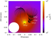 |
Fig. 5. Illustrative figure of the motion of S2 through the hot flow around Sgr A* of variable density. The density may change by as much as an order of magnitude from the apocentre to the pericentre, from several hundred particles per cubic centimetre to several thousand particles per cubic centimetre, respectively, depending on the power-law slope of the radial number density distribution. For the exemplary calculation, we used na = nB(r/rB)−1, where nB = 20.3 cm−3 is the particle density at the Bondi radius. The white circle in the bottom left corner depicts the L′-band point spread function corresponding to 8m-class telescopes, from which it is apparent that the S2 bow shock remains unresolved, especially close to the pericentre. |
As the orbital eccentricity is well constrained for S2, e = 0.885, the ratio can be estimated to be na, P/na, A ∼ 4.05, 16.39, and 66.36 for the plausible density slopes of 0.5, 1.0, and 1.5, where the first two values represent the radiatively inefficient accretion flow (see e.g. Xu et al. 2006; Wang et al. 2013) and the last value corresponds to the spherical steady Bondi flow (Różańska et al. 2015). As the variation in density is large (by a factor of 16.4) for a rather small variation in the density slope (by a factor of three), the L′-band observations of S2 can be used to constrain the density distribution of the hot accretion flow close to Sgr A* at the length scales of the order of 1500 Schwarzschild radii, where there are essentially no constraints for the ambient density (see, however, Gillessen et al. 2019).
In the further model, we approximate the orbit of S2 with an ellipse with a semimajor axis of 0.12538″≈5 mpc and an eccentricity of 0.88473 according to recent GRAVITY measurements (Gravity Collaboration 2018a). These orbital elements imply that S2 covers a large distance range, with a pericentre distance of rp = 119.2 AU = 1512 rs and an apocentre distance of ra = (1 + e)/(1 − e)rp = 16.35rp = 24724 rs. The power-law density distribution is adopted according to the Chandra X-ray studies of the extended emission of Sgr A* in the X-ray domain (Baganoff et al. 2003; Wang et al. 2013). The density distribution can be scaled with respect to the Bondi capture radius, na ≈ na, B(r/rB)−γ, where  and rB ≈ 4″(Ta/107 K)−1 = 0.16 pc (Baganoff et al. 2003; Wang et al. 2013). Figure 6 shows the number gas density per cubic centimetre (cm) that is expected to be intercepted by S2 star during its entire orbit (zero time stands for the orbit periapse). Different lines stand for different density slopes (0.5; 1.0; 1.5) according to the key. The bottom dashed red line depicts the inferred number density close to the Bondi radius according to X-ray observations of Baganoff et al. (2003), while the upper dashed red line stands for the number density of
  inferred for the periapse of the DSO/G2 object (Gillessen et al. 2019).
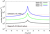 |
Fig. 6. Temporal evolution of the number density of the ambient medium for the three different density slopes of the radial density profile, na = n0(r/r0)−γ, where γ is equal to 0.5, 1.0, and 1.5; see the plot legend. The dashed red lines indicate the number densities that were observationally inferred by Baganoff et al. (2003) (26 cm−3 at the Bondi radius) and Gillessen et al. (2019) (4000 cm−3 at ∼1000 rs). |
We see that due to an eccentric orbit, S2 can in principle serve as a good probe of the ambient gaseous-dusty medium. For the S2 stellar blackbody emission, we adopt the stellar parameters that can reproduce the L′ flux density of ∼9 mJy. For the model with log(LS2/L⊙) = 4.54, TS2 = 26800 K, RS2 = 6 R⊙, we obtain the L′ flux density of FL = 8.9 mJy; see also Fig. 7 for the spectral energy distribution (SED) of S2 around L′-band.
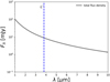 |
Fig. 7. Total SED of the S2 star (black solid line) around L′ band. |
3.1. Extinction estimate inside the Bondi radius
We assume that the ambient gas inside the Bondi radius has a power-law profile, na ≈ na, B(r/rB)−γ, which we scaled to the number density at the Bondi radius rB. To estimate the local extinction due to the gas and dust inside the Bondi radius, we calculate the local column density of hydrogen,
 (3)
(3)
where we integrated from a certain inner radius associated with S2, in this case its pericentre distance of rP = aS2(1 − eS2) ≈ 0.577 mpc, up to the Bondi radius. The column density estimate for the number density of nB ≈ 26 cm−3 (Baganoff et al. 2003) at the Bondi radius and the maximum density power-law slope of γ ≈ 1.5 for the Bondi-type flow is Nh(γ = 1.5) = 4.02 × 1020 cm−2, whereas for the flat slope of γ = 0.5, we get Nh(γ = 0.5) = 2.41 × 1019 cm−2. The visual extinction due to the ambient gas inside the Bondi radius for the steep density profile (γ = 1.5) is given by AV ≈ 5.6 × 10⁻²² Nh(cm−2) = 0.23 mag (see e.g. Reina & Tarenghi 1973; Gorenstein 1975; Predehl & Schmitt 1995), which corresponds to the extinction AK ∼ 0.1 AV = 0.023 mag in the NIR K-band and AL ≈ 0.5 AK = 0.012 mag in the NIR L′-band (see Schödel et al. 2010, for the extinction analysis towards the GC), in which our observations were carried out. For the flat density profile of γ = 0.5, we get AL ≈ 0.0007 mag. Therefore, no increase in the L′-band magnitude within uncertainties is expected from the S2 plunging in deeper towards higher ambient densities. In summary, the upper limit on the ambient extinction inside the Bondi radius is AL ≲ 0.012 mag. The only substantial increase at longer NIR wavelengths can be produced locally due to the bow-shock formation characterised by its density, radial scale, and thickness, which allows us to estimate the extinction.
3.2. Constraining the ambient density based on the thermal bow-shock emission
The S2 bow shock is modelled using a two-shock scenario (Dyson 1975), where one shock is driven into the ambient medium (ambient shock) and the other is formed from the shocked stellar wind (stellar-wind shock). These two layers are separated by a contact discontinuity at a distance approximately given by the stagnation radius; see Eq. (B.1). This treatment is based on the analytical theory of Dyson (1975), who modelled an interaction of a fast stellar wind with an expanding gas globule. In the first approximation, two layers (warm and cold) mix to form one shocked layer. In the second approximation, two layers are separated by a contact discontinuity. We apply the second approximation in a similar way to Scoville & Burkert (2013) for the GC NIR-excess source DSO/G2 interacting with the ambient diluted medium (see also their Fig. 3 for the illustration). The extinction estimate is based on the number density of gas and dust inside the shock and its characteristic length-scale, or ‘thickness’. At the stagnation point, the ambient shock is characterised by the number density nams = 4na and a thickness of tams = 0.65R0. The stellar wind shock has a characteristic number density of  , where
  is the stellar wind number density with the mean molecular weight of μ = 0.5 (ionised gas) and the hydrogen mass of mH and the sound speed of the stellar wind gas cs = (kBTsw/μmH)1/2 is evaluated for the temperature of Tsw = 104 K. The thickness of the stellar wind is given by tsws = 2.3(cs/vw)2R0. We show both the number density and the thickness of both shocks in Fig. 8 as a function of the distance of S2 from Sgr A* in Schwarzschild radii. We see that the ambient shock is thicker and less dense than the stellar wind shock for all ambient density profiles considered in the legend.
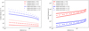 |
Fig. 8. Number density and thickness of the two shock layers in the two-shock approximation model as a function of the distance from Sgr A* (in Schwarzschild radii). Left: number density (expressed in cm−3) of the shock driven into the ambient medium (red lines) and of the shocked stellar wind (blue lines) calculated for three specific values of the ambient density slope: γ = 0.5, 1.0, and 1.5. Right: thickness (expressed in cm) of the stellar-wind (blue lines) and ambient shock layers (red lines) calculated for the three different density slopes as in the left panel. |
In our model, we further consider that the dust is more likely to exist in the ambient medium through which S2 moves along its orbit, and therefore the ambient shock is expected to be more relevant in terms of the localised extinction and its contribution in the L′-band. The B-type stars typically do not contain dust in their stellar winds, and therefore the stellar wind shock is not likely to contribute to L′-band emission. However, for completeness, we consider both shock layers in assessing the constraints on the ambient number density. This is also due to the complex dynamics of dust grains and their potential of being dragged by a denser material in the stellar-wind shock; especially smaller grains may be affected (see e.g. van Marle et al. 2011). During the motion of S2, the two shock layers are affected by hydrodynamic instabilities that lead to the mixing of both layers (Schartmann et al. 2018), which is likely to lead to the exchange of material and the actual density of the gaseous-dusty mixed layer may be closer to the denser stellar-wind shock.
We calculate the limits on the ambient number density at the S2 periapse as well as the limits for the density slope γ. The upper limit is obtained if we associate the upper limit for the extinction with the standard deviation, Ashock ≲ 0.04 mag. Another estimate is based on the fractional variability with Ashock ∼ 0.02 mag. The values of the density and the slope are inferred from the extinction-column density relation AV ≈ 5.6 × 10⁻²² Nh(cm−2), where Nh ∼ nshocktshock with the shock number density nshock and a shock thickness tshock for each shock layer as explained above. The extinction in L′-band is approximately given by AL = 0.5 × 0.1 × AV (Schödel et al. 2010). This model allows us to compute the whole light curve along the S2 trajectory. In Table 2, we list the density slope and the number density constraints for each extinction value, with the shock layer taken into account. For the ambient shock, which is more likely to lead to an increased dust emission, the upper limits on the number density are in the range  with the density slope γ ≲ 3.03−3.20. For the stellar-wind shock, the number densities are smaller by four orders of magnitude and the density slope is smaller by a factor of two,
  and γ ≲ 1.41−1.57.
Summary of constraints for the ambient density close to the GC at the S2 periapse based on the two extinction limits, 1σ and fractional variability, and analytical bow-shock models for both the ambient shock and the stellar-wind shock thermal emission.
Figure 9 shows a comparison of model light curves with the actual L′-band data, with the upper panels representing the larger extinction value of A = 0.04 based on the standard deviation of the light-curve points and the lower panels showing results with the smaller extinction of A = 0.02 based on the fractional variability. The peak of the observed light curve has an apparent offset from the peak of the modelled light curves (at the periapse), which is most likely a systematic effect and not an intrinsic brightening.
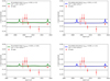 |
Fig. 9. Comparison of model light curves based on the mean S2 emission and the modelled thermal emission of its bow shock (solid green and blue lines) with the observed L′-band emission of S2 (red points with errorbars). Upper panels: modelled thermal emission of the bow shock is associated with the extinction of A = 0.04 mag, which was inferred from the standard deviation of observed light curve points. We model the thermal dust emission of the ambient bow shock (solid green line in left panel) and the thermal emission of the stellar-wind shock (solid blue line in right panel) separately. The horizontal solid black line represents the light curve mean value, while the dashed black lines stand for the standard deviation. Lower panels: as in the upper panels, but for the extinction of A = 0.02 mag based on the excess variance of the observed light-curve points. |
3.3. Constraining the ambient density based on the non-thermal bow-shock emission
The thermal bow-shock emission in L′-band is clearly affected by the presence of dust along the S2 orbit. While on one hand the dust is clearly present in dusty objects whose orbits lie in the S cluster, the hot ambient medium likely destroys the dust particles continually. In cases where the presence of dust is diminished along the S2 orbit, the thermal emission of the bow shock in the L′-band is even smaller than we predicted in Sect. 3.2.
Another way to constrain the ambient density at the S2 pericentre is to take into consideration the broadband non-thermal synchrotron emission of the bow shock, which does not depend on the presence of dust. When the bow shock develops ahead of the star, it provides a volume where electrons can be accelerated by the enhanced magnetic field. Subsequently, they cool off by emitting synchrotron emission. Ginsburg et al. (2016) used the same mechanism to claim that the non-thermal emission of stellar bow shocks in the S cluster may be comparable to the radio and NIR emission of Sgr A*, and therefore could be detected.
One can reverse the task and instead constrain the upper limit of the ambient density based on the statistical variations we detect in the L′-band light curve of S2. According to Table 1, the maximum flux difference in our light curve is 0.90 mJy, while the rms fractional variability is at the level of 0.2 mJy. Therefore, the maximum contribution of the bow-shock synchrotron emission in L′-band can only be at this flux density level, which allows us to place an upper limit on the ambient density.
For the calculation of the bow-shock synchrotron light curve and broad-band spectrum, we follow the model of Sądowski et al. (2013), originally developed for the estimate of the bow-shock emission of the DSO/G2 object; see also Zajaček et al. (2016). As in Sądowski et al. (2013) and Zajaček et al. (2016), for calculating synchrotron light curves and spectra, we use the temperature profile of the ADAF, Ta = 9.5 × 10¹⁰(r/rs)−1 (Yuan et al. 2003), with the ratio between the magnetic and the gas pressure of χ = Pmag/Pgas = 0.3, and the Mach number of the star at the pericentre distance of S2, ℳ = 2.6. Other relevant parameters were adopted from particle-in-cell simulations performed by Sądowski et al. (2013); specifically, the slope of the high-energy power-law electron distribution, p = 2.4, the minimum Lorentz factor, ζ = 7.5, and the fraction of accelerated electrons to high energies, η = 0.05. Specifically for S2, we used its mass-loss rate ṁw ≃ 3 × 10⁻⁷ M⊙ yr−1 and the terminal wind velocity vw ∼ 103 km s−1 inferred from spectroscopy (Martins et al. 2008; Habibi et al. 2017).
In contrast to Sądowski et al. (2013), we perform only the plowing synchrotron model, in which the accelerated electrons are kept in the shocked region and radiate in the shocked magnetic field. The plowing model is more likely to contribute in L′-band than the local model, in which accelerated electrons leave the shock and radiate in the unshocked magnetic field. Due to the short cooling time for the NIR L′-band synchrotron emission, tcool ≈ 0.25(B/0.08 G)−3/2(νc/8 × 1013 Hz)−1/2 yr, the local model would have a negligible contribution.
In Fig. 10 (left panel), we plot the L′-band synchrotron light curve for the peak flux density of 0.91 mJy, which corresponds to the maximum flux difference, and the light curve with the peak flux density of 0.22 mJy, which corresponds to the fractional variability. The non-thermal bow-shock emission is also compared with the Sgr A* mean flux density in L′-band (Schödel et al. 2011), the S2 total flux, and the actual S2 measured flux density from 2018.307, which are all larger by at least a factor of a few than the bow-shock non-thermal emission. In the right panel of Fig. 10, we plot the SED of the S2 bow-shock synchrotron emission calculated for the pericentre for both L′-band flux density values (maximum difference and fractional variability). We also compare the synchrotron bow-shock SED with the SED of Sgr A* calculated using the advection-dominated accretion flow model (ADAF; Yuan et al. 2003; Yuan & Narayan 2014). Taking into account the maximum flux difference as an upper limit for the L′-band synchrotron contribution, we get the pericentre number density of na = 1.01 × 105 cm−3 (the slope of 1.47). The fractional variability flux limit yields the number density of 1.88 × 104 cm−3 (the density slope of 1.17). Both limiting cases are summarised in Table 2. For both density limits, the bow-shock synchrotron flux density would be comparable to that of Sgr A* at frequencies of a few GHz, where the peak of its SED occurs. To separate Sg A* and the predicted S2 bow-shock emission is challenging as it requires highly sensitive measurements at cm to decimetre (dm) wavelengths with an angular resolution of a tenth of an arcsecond or better. However, around the time of the periapse passage, long-term (weeks to a few months) light curves should reveal an overall increase of the spatially unresolved emission of both sources. Such a data set is not available at present. Very-long-baseline interferometry (VLBI) measurements at GHz frequencies (or cm wavelengths) could in principle be possible due to the high brightness temperature of the S2 bow-shock emission at its pericentre. We outline here a few basic estimates. For the assumed maximum non-thermal excess in L′-band of ∼1 mJy, the calculated peak of the bow-shock synchrotron spectrum is at 4.61 GHz. The peak flux density is expected to be 0.86 Jy at the S2 pericentre, which is comparable to or even larger than the flux density of Sgr A* at cm wavelengths. The characteristic size of the bow shock given by the stagnation distance would be R0 ∼ 5.6 × 1013 cm at the pericentre, which gives the angular scale of ∼0.5 mas, which is below the resolution capabilities of the cm VLBI, namely ∼1 mas at best. The angular distance between the S2 radio source and Sgr A* at the pericentre is ∼14.4 mas, which is smaller than the intrinsic size of Sgr A* at 6 cm (∼20 mas), because of λ2 scatter-broadening of the size of Sgr A* (Bower et al. 2006; Doeleman et al. 2008). The brightness temperature2 of the S2 bow shock at its pericentre would be large, TB ∼ 8.5 × 10¹⁰ K, comparable to that of Sgr A*, ≳2 × 10¹⁰ K (Krichbaum et al. 1998; Doeleman et al. 2008). However, before and after the S2 pericentre, its brightness temperature is expected to drop rather fast, remaining above 106 K from the epoch 2017.08 up to 2020.54, with the peak at the pericentre in 2018.38. Taking into account the smaller contribution of S2 bow-shock non-thermal emission at L′-band at the level of ∼0.2 mJy, which results from a smaller ambient density, mainly the characteristic size is affected; it increases to R0 = 1.29 × 1014 cm, which corresponds to the angular scale of 1.1 mas, which is at the limit of the resolving power of the cm VLBI. However, as for a lower density the resulting spectrum of the S2 bow shock is shifted towards the lower frequency at 1.5 GHz (see Fig. 10), the bow-shock size is actually smaller than the typical VLBI beam FWHM of ∼3″. With the peak flux of 435 mJy, the brightness temperature of TB ∼ 7 × 10¹⁰ K is again comparable to that of Sgr A* and remains above 106 K in the time window between 2016.98 and 2020.90. In general, the cm VLBI observations could reveal a deviation from the Gaussian core of Sgr A* in the epochs of ∼1.5 years before and after the pericentre when the brightness temperature is still above 106 K. At the pericentre, it is not possible to resolve the S2 bow-shock emission because of the scatter-broadening of Sgr A* and the bow-shock source. Only the flux excess could be detected; however, in that case a corresponding light curve at cm wavelengths would need to be analysed to distinguish the long-term bow-shock excess from the short-term stochastic radio flares.
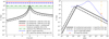 |
Fig. 10. Non-thermal contribution of the S2 bow shock to its L′-band emission. In the left panel, we plot the L′-band light curve as calculated for the S2 bow-shock synchrotron emission for the peak flux of 0.91 mJy (solid black line) and for the peak flux of 0.22 mJy (dashed black line). For comparison, we also show the fractional variability of S2 (dotted green line) and its maximum flux difference (dot-dashed line). The measured mean flux of Sgr A* in L′-band, 4.33 ± 0.18 mJy, is depicted by a dashed blue line. The sum of the mean flux density of S2 with the maximum potential contribution of the non-thermal bow-shock emission is represented by a solid red line. The measured flux density of S2 from 2018.307 is marked by an orange cross. In the right panel, we show the SED of S2 bow-shock synchrotron emission as calculated for the S2 pericentre for the L′-band flux of 0.91 mJy (solid line) and for the L′-band flux of 0.22 mJy (dashed line). The orange dot-dashed line marks the L′-band frequency range and the red star symbol represents the mean flux density of S2 in L′-band. The blue solid line represents the SED of Sgr A* based on the advection dominated accretion flows (ADAFs; Yuan et al. 2003; Yuan & Narayan 2014). |
Based on the upper limit inferred from the maximum synchrotron contribution to the L′-band emission of S2, accretion flows exceeding the particle density of ∼105 cm−3 at ∼1500 rs are unlikely. On the other hand, the presence of the Bondi-type flow with γ ∼ 3/2 cannot be excluded based on our L′-band light-curve analysis.
4. Discussion
Our observational analysis of the L′-band emission of the star S2 yields a light curve that is essentially flat within uncertainties and shows intrinsic flux variations due to the interaction of S2 with the ambient medium or due to intrinsic stellar variability at the level of ∼2.5% only, as given by the fractional variability. Using the theory of a two-layer bow shock (Dyson 1975), we are therefore only able to place an upper limit on the ambient density at the S2 periapse as well as an upper limit on the density slope. The upper limit considering the contribution of the ambient bow shock, which is more likely to contain dust, is na ≲ 1.87 × 109 cm−3, and the upper limit for the slope is γ ≲ 3.20. These values change only slightly when one considers the smaller extinction of (A = 0.02) as indicated by the excess variance, na ∼ 7.15 × 108 cm−3 and γ = 3.03. If the stellar-wind shock layer were found to contain dust, which would require the turbulence and the mixing of shocked layers, then the density and the slope constraints would decrease to na = 7.53 × 10⁴ − 1.86 × 105 cm−3 and γ = 1.41−1.57. The non-thermal synchrotron emission of the bow-shock appears to put tighter constraints on the S2 pericentre density: na ≲ 1.01 × 105 cm−3 for the maximum flux difference and na ≲ 1.88 × 104 cm−3 for the fractional variability. For the slope, we obtain γ ≲ 1.47 for the maximum flux difference and γ ≲ 1.17 for the fractional variability.
Therefore, the L′-band data is consistent with the S2 star interacting with a hot, diluted ambient flow with a power-law density slope of γ ∼ 0.5 (generally the advection-dominated flow (ADAF); Wang et al. 2013) and with a spherical Bondi-type solution with a density slope of γ ∼ 1.5 (also consistent with the convection-dominated flow (CDAF); Różańska et al. 2015). Moreover, we cannot exclude the possibility that S2 interacts with an even denser and colder type of medium, such as the proposed cool disc with densities in the interval of nCD ∼ 105 − 106 cm−3 (Murchikova et al. 2019). Indeed, the uppermost limit for the density na < 1.87 × 109 cm−3 is well in the range for the number density of broad-line region (BLR) clouds nBLR ∼ 108 − 1011 cm−3 (Gaskell 2009). Although we do not expect the presence of BLR clouds in such a low-luminosity nucleus as Sgr A* (see, however, Bianchi et al. 2019 for the discovery of the compact BLR in the low-luminosity Seyfert galaxy NGC3147 with L/LEdd ∼ 10−4), we cannot exclude the presence of denser gaseous-dusty structures, with which stars can occasionally interact, such as dust-enshrouded objects monitored in the S-cluster (Peißker et al. 2020b; Ciurlo et al. 2020). This is also supported by the multiphase medium of Sgr A* on the scale of one parsec (Moser et al. 2017), which could also be present on smaller scales due to for example thermal instability (Różańska et al. 2017). In particular, Peißker et al. (2020a) report a detection of the proper motion of a Brγ filament, whose estimated distance is close to the Bondi radius at ∼0.2 pc. At comparable scales, Royster et al. (2019) used the H30α line to trace a blueshifted, ionised gas with a velocity of between −480 and −300 km s−1, which appears to be outflowing. Hence, the environment close to the Bondi radius is complex in terms of both kinematics and density.
Based on the flat L′-band light curve and the upper limits on the density, we can exclude the presence of a cold, thin accretion disc (Shakura & Sunyaev 1973), whose number densities close to the periapse of S2 at ∼1500 rs can be estimated using the relation for the number density as given by the standard accretion disc theory; see also Frank et al. (2002). Using the mean atomic weight of μ = 0.615 for the fully ionised gas, we obtain
 (4)
(4)
where the factor f stands for f = [1 − (rs/R)1/2]1/4. We calculate a number density range of ndisc = 7.6 × 10¹¹ − 9.6 × 1012 cm−3 for the accretion rate in the range ṁ = 10−9 − 10−7 M⊙ yr−1 and a viscous parameter of α = 0.1 for the S2 pericentre distance. In Fig. 11, we plot the thin disc density profiles up to 100 rs, since the density profile below this radius is relatively uncertain and the accretion flow likely breaks up due to the accumulation of poloidal magnetic flux, which results in a magnetically arrested disc (MAD; Narayan et al. 2003). This transition occurs where the magnetic energy density and the gravitational potential energy are at balance, B2/8π = GM•ρflow/Rm, from which we can easily derive the magnetospheric radius,
 (5)
(5)
 (6)
(6)
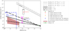 |
Fig. 11. Comparison of the upper density limits that are marked as downward arrows inferred from the L′-band light curve of the S2 star based on modelling ambient and stellar-wind shocks for the dust-extinction values of 0.04 and 0.02 mag with different density profiles and structures according to the plot legend and the description. Alongside the density limit based on the thermal bow-shock emission, we also depict the limit based on the non-thermal bow-shock emission (bluish downward arrows). For comparison, we show the density limit of 26 cm−3 inferred by Baganoff et al. (2003) based on the analysis of the X-ray thermal bremsstrahlung profile. Then we show the density constraint of (5 ± 3) × 103 cm−3 inferred from the potential hydrodynamic drag acting on the DSO/G2 object (Gillessen et al. 2019). The general density power-law profiles are depicted by black lines: the solid line stands for the slope of 1.0, the dashed line represents the flat profile of γ = 0.5, and the dot-dashed line depicts the steeper Bondi-like spherical flow with γ = 1.5. The shaded rectangle shows the distance and the density limits (n ∼ 105 − 106 cm−3) of the putative cool disc whose discovery is claimed by Murchikova et al. (2019). The black-framed rectangle depicts the typical densities of the broad-line region (BLR) clouds in the range of n ∼ 108 − 1011 cm−3. The gray lines depict the number density values expected for a thin disc (Shakura & Sunyaev 1973) for the accretion rate of Ṁ = 10−9 − 10−7 M⊙ yr−1 and the viscosity parameter of α = 0.1. The brown-shaded area to the lower left shows the set of density profiles determined using the rotation measure of the submillimeter polarisation measurements (Marrone et al. 2006, 2007) for the inner radii of rin = 300 rs and rin = 3 rs, density slopes of γ = 0.5−1.5, and the accretion rates in the range 2 × 10⁻⁹ − 2 × 10⁻⁷ M⊙ yr−1. The blue dot-dashed vertical at 100 rs and the blue dot-dashed arrow to the left denote the region of a potential magnetically arrested flow (MAD), where the accretion flow changes from continuous to clumpy due to the accumulated poloidal magnetic flux (see e.g. Narayan et al. 2003; Tursunov et al. 2020). The dotted vertical lines mark the periapsis of the S62 star at ∼225 rs and the periapsis of the S2 star at ∼1512 rs. Next to the S2 pericentre vertical line, we highlight the range of densities potentially being explored using L′-band METIS at ELT imaging mode. |
where the poloidal magnetic field is scaled to 10 G and the number density of the flow to 106 cm−3 according to the synchrotron models of the Sgr A* flares (Yusef-Zadeh et al. 2006; Eckart et al. 2012). The putative MAD part of the flow is highlighted by the blue vertical line in Fig. 11.
The thin disc is expected to contain dust from the sublimation radius towards larger distances. If we associate the effective thin disc temperature, Teff = [3GM∙ṁ/(8πr3σB)]1/4, with the dust sublimation temperature of Tsub = 1000 K, we get a relation for the dust sublimation radius (see also Czerny & Hryniewicz 2011)
 (7)
(7)
We obtain the range of rsub = 35−163 rs for the accretion rate range of ṁ = 10−9 − 10−7 M⊙ yr−1. Hence, the dusty bow-shock layer should be formed when the S2 plunges through the disc midplane close to its periapse at ∼1500 rs. The formation of the shock in the disc material would lead to the extinction increase in L′-band magnitude by 0.65 mag for the density of 4.9 × 1011 cm−3 and by as much as 2.30 mag for the density of 6.13 × 1012 cm−3. We can therefore exclude the possibility that the S2 star crosses a thin, dense, and cold disc.
Although the comparison with the thin disc density in Fig. 11 may seem purely academic for the Sgr A* environment, it is still instructive to compare our upper limits with the thin-disc density for two reasons. Firstly, although the presence of a thin disc was implicitly excluded already based on X-ray and mm observations (Yuan et al. 2003; Baganoff et al. 2003; Dexter et al. 2010), the upper density limit inferred from the stellar bow shock is independent of these previous measurements. Secondly, the transition between the hot advection-dominated accretion flows (ADAFs) and thin discs at such low accretion-rate values, such as those for Sgr A*, is still not well understood. For α discs, the viscously stable branch at low ṁ exists in the stability curve of surface density–accretion rate or Σ-ṁ plot and these discs would be both geometrically and optically thin; see e.g. Frank et al. (2002). Furthermore, they would primarily cool via the free-free emission instead of black-body radiation (Tylenda 1981) and one of the main reasons why such a disc is likely not present for Sgr A* is the short time for plasma to cool down via bremsstrahlung due to the low-angular momentum of the flow. On the other hand, they are low accretion-rate systems where the thin disc was detected, such as for example the maser source NGC4258 (Gammie et al. 1999) and NGC3147 (Bianchi et al. 2019). Most likely, the boundary conditions of the flow, that is, either feeding by stellar winds or the inflow of gas from larger scales, determine the transition between the ADAF and the thin disc at low ṁ and vice versa. In addition, hybrid models of discs have been suggested, with an outer thin disc part and an inner hot ADAF part, with the transition at 10–100 gravitational radii (Gammie et al. 1999).
In order to better constrain the density and lower the upper density limit and the slope, the photometry precision needs to improve, with values below 0.01 mag. Also, a more precise theory for the bow shock formation and its corresponding NIR emission needs to be taken into account. However, the current methodology that we provide here can be directly transferred to the more precise photometry.
In terms of future instruments, the METIS at ELT will be particularly well suited for high-precision photometry in near- and mid-IR domains. All observing modes of METIS will initially work with a single conjugate adaptive optics (SCAO) system at or close to the diffraction limit of the 39m ELT. At a wavelength of 3.5 μm, the ELT will allow operation at an angular resolution of 23 milliarcseconds. Here, METIS will have a point source sensitivity (10-σ in 1 hour) of 21.2 mag (or about 1 μJy) (Brandl et al. 2018a,b). In the N band at a wavelength around 10 μm, the point-source sensitivity can be expected to be about 1.6 orders of magnitude lower. The field of view of about 10″ × 10″ in imaging and 1.0″ × 0.5″ in IFU (integral field unit) spectroscopy mode at L- and M-bands is ideally suited for the densely populated GC region. However, the limiting sensitivity for flux density measurements in this field will be determined by confusion due to source crowding. Hence, the effective sensitivity available to determine flux densities and to establish light curves can safely be assumed to be an order of magnitude lower than the nominal point-source sensitivity, but will still be about an order of magnitude better than the currently reached sensitivity. For specific estimates of the potentially probed density range, we consider the limiting flux density value for the bow-shock emission in the L′-band to be 0.01 mJy, which corresponds to an ∼10−3 mag difference in the S2 star L′-band magnitude. Taking into account the model of thermal ambient-shock emission, which is the least sensitive in terms of the density, we obtain a value of ∼1.5 × 106 cm−3. This provides an improvement by three orders of magnitude in comparison to the current upper limit. The more sensitive non-thermal bow-shock emission model implies a lower ambient-density limit of only ∼700 cm−3, which is two orders of magnitude lower than current limits in Table 2. The density range probed by METIS is also shown specifically in the summary plot in Fig. 11. In particular, using the lower limit of 700 cm−3 inferred from the non-thermal model, METIS should be able to directly detect a non-thermal emission increase in case the hot-flow slope is larger than γ = 0.5 between the Bondi radius and the S2 pericentre distance. Further details will have to be determined through observations on the target.
The next-best target to observe both the potential thermal and non-thermal bow-shock emission at the periapse would be S62 in early 2023 which appears to be a suitable time to observe the closest S-star to the SMBH by the JWST. This will be an opportunity to shed further light on the density of the accretion flow around Sgr A* along the S62 orbital plane (Peißker et al. 2020c), in particular at its pericentre distance of  , where the conditions of the accretion flow were only constrained via the rotation measure (Marrone et al. 2006, 2007); see Fig. 11. The detection of the bow-shock emission of S62 would provide an independent means of assessing the ambient number density on the scale of ∼100 rs. Furthermore, the S stars S2 and S62 as well as the dusty source DSO/G2 orbit Sgr A* at different inclinations. Therefore, detecting the bow-shock emission for each of them would enable us to constrain the density profile of the accretion flow around Sgr A* not only as a function of distance, but for a broader range of inclinations.
NIR bow-shock emission from the S stars, which is expected to be most prominent at the pericentre, could be detected via peculiar, longer Ks or L′-band flares. Moreover, the total bow-shock flare duration would be of the order of a few months up to one year and the peak flux is coincident with the pericentre of the star, see our model predictions in Fig. 9 for the thermal dust emission and in Fig. 10 for the non-thermal synchrotron emission associated with the bow shock. The start of the flux increase would be half a year before the pericentre. In terms of the shocked stellar wind, Giannios & Sironi (2013) and Christie et al. (2016) calculated the timescale of approximately one month for the X-ray bremsstrahlung flare produced by S2 bow-shock with the luminosity of 4 × 1033 erg s−1. However, Schartmann et al. (2018) argued that for the expected accretion-flow density, the X-ray emission from the bow shock is beyond the detection limit. Ginsburg et al. (2016) calculated the non-thermal synchrotron emission, which for the typical parameters assumed for S2, the mass-loss rate of ṁw ∼ 10−7 M⊙ yr−1 and the terminal wind velocity of vw ∼ 103 km s−1, is below the quiescent emission of Sgr A*. Therefore, the stochastic IR flares of Sgr A* (Witzel et al. 2012, 2018), including the very bright ones (Do et al. 2019b), are not associated with the stellar bow shocks in the S cluster as they evolve on a timescale of several hours only, which can be interpreted as an orbital timescale of plasmoids close to the innermost stable circular orbit (Gravity Collaboration 2018b). In other words, some short-term NIR flares could be associated with short-period stars orbiting Sgr A* on the scale of the innermost stable circular orbit (Leibowitz 2020), which could be disentangled from the stochastic background via their periodic or quasi-periodic signal. However, the bright IR flare analysed by Do et al. (2019b) could be associated with a change of accretion state due to the recent pericentre passage of S2 in 2018 or even the pericentre passage of DSO/G2 in 2014. The time delay between the pericentre and the average flare statistics may be interpreted via the viscous timescale of the hot accretion flow, which can be of the order of one to ten years (Czerny et al. 2013).
5. Conclusions
For the brightest star in the S cluster, S2, we obtained a light curve in the NIR L′-band, which is flat within the measurement uncertainties with the fractional flux variability of only 2.52% in terms of the L′-band flux density. When we associate the flux density standard deviation of 0.04 mag with the local dust extinction due to the bow shock, we can place an upper limit of na < 1.87 × 109 cm−3 on the ambient number density at ∼1500 rs for the warm bow shock driven into the ambient medium, which is expected to contain dust. For the colder and the denser stellar-wind shock, the number density limit is na < 1.86 × 105 cm−3, which is nevertheless less firm because of the limited presence of dust in stellar winds of B-type stars. Considering the non-thermal bow-shock emission, which does not rely on the existence of dust, we can place an upper density limit of 1.01 × 105 cm−3.
These limits cannot yet constrain the type of the hot accretion flow and therefore both the radiatively inefficient accretion flow with the density profile of γ = 0.5 and the spherical Bondi-type flow with γ = 1.5 can accommodate these number densities. However, we can firmly exclude the standard, thin accretion disc extending all the way to 1 500 rs, the density of which would be at least two orders of magnitude greater and the star-disc interactions would produce a shock with a local extinction of 0.65−2.30 mag in L′ band, which is much larger than the inferred 1σ excess of 0.04 mag of the L′-band light curve, and a difference of 0.11 mag between the maximum and the minimum magnitude.
In terms of future prospects, a major challenge is to detect and directly resolve bow shocks associated with the S-stars in NIR bands because of the high confusion and stellar density close to Sgr A*. It may become possible when high-resolution mid-IR imaging becomes available with the next generation of instruments, namely METIS at the ELT, because bow shocks are generally more prominent because of the dust emission in mid-IR bands. High-precision photometry associated with METIS with the flux sensitivity of the ∼0.01 mJy in L′-band is expected to improve the density constraints by two to three orders of magnitude in comparison with our current upper limits. For the non-thermal bow-shock emission, the direct detection of the flux excess is plausible in cases where the hot-flow density slope is larger than γ ∼ 0.5 between the Bondi radius and the S2 pericentre distance.
The S2 pericentre distance according to Gravity Collaboration (2018a) is 1513 Schwarzschild radii.
We estimate the brightness temperature using the standard relation derived from the Rayleigh-Jeans approximation in the radio domain,  , where the solid angle
  with R0 being the stagnation radius of the bow shock.
We use the indices P, A, and 90° to denote the quantities evaluated at the pericentre, apocentre, and the semi-latus rectum, respectively.
Acknowledgments
The authors would like to thank the referee for his/her constructive suggestions and Persis Misquitta for the diligent proofreading of this paper. S. Elaheh Hosseini is a member of the International Max Planck Research School for Astronomy and Astrophysics at the Universities of Bonn and Cologne. We thank the Collaborative Research Centre 956, sub-project A02, funded by the Deutsche Forschungsgemeinschaft (DFG) – project ID 184018867. Michal Zajacek acknowledges the financial support from the National Science Centre, Poland, grant No. 2017/26/A/ST9/00756 (Maestro 9).
References
- Agol, E. 2000, ApJ, 538, L121 [NASA ADS] [CrossRef] [Google Scholar]
- Aitken, D. K., Greaves, J., Chrysostomou, A., et al. 2000, ApJ, 534, L173 [Google Scholar]
- Alexander, T. 2005, Phys. Rep., 419, 65 [NASA ADS] [CrossRef] [Google Scholar]
- Baganoff, F. K., Maeda, Y., Morris, M., et al. 2003, ApJ, 591, 891 [NASA ADS] [CrossRef] [Google Scholar]
- Bianchi, S., Antonucci, R., Capetti, A., et al. 2019, MNRAS, 488, L1 [NASA ADS] [CrossRef] [Google Scholar]
- Boehle, A., Ghez, A. M., Schödel, R., et al. 2016, ApJ, 830, 17 [NASA ADS] [CrossRef] [Google Scholar]
- Borkar, A., Eckart, A., Straubmeier, C., et al. 2016, MNRAS, 458, 2336 [NASA ADS] [CrossRef] [Google Scholar]
- Bower, G. C., Wright, M. C. H., Falcke, H., & Backer, D. C. 2003, ApJ, 588, 331 [Google Scholar]
- Bower, G. C., Goss, W. M., Falcke, H., Backer, D. C., & Lithwick, Y. 2006, ApJ, 648, L127 [NASA ADS] [CrossRef] [Google Scholar]
- Bower, G. C., Markoff, S., Dexter, J., et al. 2015, ApJ, 802, 69 [NASA ADS] [CrossRef] [Google Scholar]
- Brandl, B. R., Absil, O., Agócs, T., et al. 2018a, in Proc. SPIE, SPIE Conf. Ser., 10702, 107021U [Google Scholar]
- Brandl, B. R., Quanz, S., Snellen, I., et al. 2018b, in The Cosmic Wheel and the Legacy of the AKARI Archive: From Galaxies and Stars to Planets and Life, eds. T. Ootsubo, I. Yamamura, K. Murata, T. Onaka, et al., 41 [Google Scholar]
- Broderick, A. E., Fish, V. L., Doeleman, S. S., & Loeb, A. 2011, ApJ, 735, 110 [NASA ADS] [CrossRef] [Google Scholar]
- Christie, I. M., Petropoulou, M., Mimica, P., & Giannios, D. 2016, MNRAS, 459, 2420 [NASA ADS] [CrossRef] [Google Scholar]
- Ciurlo, A., Campbell, R. D., Morris, M. R., et al. 2020, Nature, 577, 337 [NASA ADS] [CrossRef] [Google Scholar]
- Clénet, Y., Rouan, D., Gendron, E., et al. 2004, A&A, 417, L15 [NASA ADS] [CrossRef] [EDP Sciences] [Google Scholar]
- Crumley, P., & Kumar, P. 2013, MNRAS, 436, 1955 [NASA ADS] [CrossRef] [Google Scholar]
- Czerny, B., & Hryniewicz, K. 2011, A&A, 525, L8 [NASA ADS] [CrossRef] [EDP Sciences] [Google Scholar]
- Czerny, B., Kunneriath, D., Karas, V., & Das, T. K. 2013, A&A, 555, A97 [NASA ADS] [CrossRef] [EDP Sciences] [Google Scholar]
- Dexter, J., Agol, E., Fragile, P. C., & McKinney, J. C. 2010, ApJ, 717, 1092 [NASA ADS] [CrossRef] [Google Scholar]
- Do, T., Witzel, G., Gautam, A. K., et al. 2019a, ApJ, 882, L27 [NASA ADS] [CrossRef] [Google Scholar]
- Do, T., Hees, A., Ghez, A., et al. 2019b, Science, 365, 664 [NASA ADS] [CrossRef] [Google Scholar]
- Dodds-Eden, K., Porquet, D., Trap, G., et al. 2009, ApJ, 698, 676 [NASA ADS] [CrossRef] [Google Scholar]
- Doeleman, S. S., Weintroub, J., Rogers, A. E. E., et al. 2008, Nature, 455, 78 [NASA ADS] [CrossRef] [PubMed] [Google Scholar]
- Dyson, J. E. 1975, Ap&SS, 35, 299 [NASA ADS] [CrossRef] [Google Scholar]
- Eckart, A., Schödel, R., García-Marín, M., et al. 2008, A&A, 492, 337 [NASA ADS] [CrossRef] [EDP Sciences] [Google Scholar]
- Eckart, A., García-Marín, M., Vogel, S. N., et al. 2012, A&A, 537, A52 [NASA ADS] [CrossRef] [EDP Sciences] [Google Scholar]
- Eckart, A., Mužić, K., Yazici, S., et al. 2013, A&A, 551, A18 [NASA ADS] [CrossRef] [EDP Sciences] [Google Scholar]
- Eckart, A., Hüttemann, A., Kiefer, C., et al. 2017, Found. Phys., 47, 553 [NASA ADS] [CrossRef] [Google Scholar]
- Eisenhauer, F., Schödel, R., Genzel, R., et al. 2003, ApJ, 597, L121 [NASA ADS] [CrossRef] [Google Scholar]
- Frank, J., King, A., & Raine, D. J. 2002, Accretion Power in Astrophysics: Third Edition (Cambridge, UK: Cambridge University Press) [Google Scholar]
- Fritz, T. K., Gillessen, S., Dodds-Eden, K., et al. 2011, ApJ, 737, 73 [NASA ADS] [CrossRef] [Google Scholar]
- Gammie, C. F., Narayan, R., & Blandford, R. 1999, ApJ, 516, 177 [NASA ADS] [CrossRef] [Google Scholar]
- Gaskell, C. M. 2009, New Astron. Rev., 53, 140 [NASA ADS] [CrossRef] [Google Scholar]
- Genzel, R., Schödel, R., Ott, T., et al. 2003, Nature, 425, 934 [CrossRef] [PubMed] [Google Scholar]
- Genzel, R., Eisenhauer, F., & Gillessen, S. 2010, Rev. Mod. Phys., 82, 3121 [NASA ADS] [CrossRef] [Google Scholar]
- Ghez, A. M., Hornstein, S. D., Lu, J. R., et al. 2005, ApJ, 635, 1087 [NASA ADS] [CrossRef] [Google Scholar]
- Ghez, A. M., Salim, S., Weinberg, N. N., et al. 2008, ApJ, 689, 1044 [NASA ADS] [CrossRef] [Google Scholar]
- Giannios, D., & Sironi, L. 2013, MNRAS, 433, L25 [NASA ADS] [CrossRef] [Google Scholar]
- Gillessen, S., Eisenhauer, F., Trippe, S., et al. 2009, ApJ, 692, 1075 [NASA ADS] [CrossRef] [Google Scholar]
- Gillessen, S., Genzel, R., Fritz, T. K., et al. 2012, Nature, 481, 51 [NASA ADS] [CrossRef] [Google Scholar]
- Gillessen, S., Plewa, P. M., Eisenhauer, F., et al. 2017, ApJ, 837, 30 [NASA ADS] [CrossRef] [EDP Sciences] [Google Scholar]
- Gillessen, S., Plewa, P. M., Widmann, F., et al. 2019, ApJ, 871, 126 [NASA ADS] [CrossRef] [Google Scholar]
- Ginsburg, I., Wang, X., Loeb, A., & Cohen, O. 2016, MNRAS, 455, L21 [NASA ADS] [CrossRef] [Google Scholar]
- Gorenstein, P. 1975, ApJ, 198, 95 [NASA ADS] [CrossRef] [Google Scholar]
- Gravity Collaboration (Abuter, R., et al.) 2018a, A&A, 615, L15 [NASA ADS] [CrossRef] [EDP Sciences] [Google Scholar]
- Gravity Collaboration (Abuter, R., et al.) 2018b, A&A, 618, L10 [NASA ADS] [CrossRef] [EDP Sciences] [Google Scholar]
- Gravity Collaboration (Abuter, R., et al.) 2019, A&A, 625, L10 [NASA ADS] [CrossRef] [EDP Sciences] [Google Scholar]
- Gravity Collaboration (Abuter, R., et al.) 2020, A&A, 636, L5 [CrossRef] [EDP Sciences] [Google Scholar]
- Habibi, M., Gillessen, S., Martins, F., et al. 2017, ApJ, 847, 120 [NASA ADS] [CrossRef] [Google Scholar]
- Krichbaum, T. P., Graham, D. A., Witzel, A., et al. 1998, A&A, 335, L106 [NASA ADS] [Google Scholar]
- Leibowitz, E. 2020, ApJ, 896, 74 [CrossRef] [Google Scholar]
- Marrone, D. P., Moran, J. M., Zhao, J.-H., & Rao, R. 2006, ApJ, 640, 308 [NASA ADS] [CrossRef] [Google Scholar]
- Marrone, D. P., Moran, J. M., Zhao, J.-H., & Rao, R. 2007, ApJ, 654, L57 [NASA ADS] [CrossRef] [Google Scholar]
- Martins, F., Gillessen, S., Eisenhauer, F., et al. 2008, ApJ, 672, L119 [NASA ADS] [CrossRef] [Google Scholar]
- Menten, K. M., Reid, M. J., Eckart, A., & Genzel, R. 1997, ApJ, 475, L111 [NASA ADS] [CrossRef] [Google Scholar]
- Merritt, D. 2013, Dynamics and Evolution of Galactic Nuclei (Princeton: Princeton University Press) [Google Scholar]
- Moser, L., Sánchez-Monge, Á., Eckart, A., et al. 2017, A&A, 603, A68 [NASA ADS] [CrossRef] [EDP Sciences] [Google Scholar]
- Murchikova, E. M., Phinney, E. S., Pancoast, A., & Blandford, R. D. 2019, Nature, 570, 83 [NASA ADS] [CrossRef] [Google Scholar]
- Nandra, K., George, I. M., Mushotzky, R. F., Turner, T. J., & Yaqoob, T. 1997, ApJ, 476, 70 [NASA ADS] [CrossRef] [Google Scholar]
- Narayan, R., Mahadevan, R., Grindlay, J. E., Popham, R. G., & Gammie, C. 1998, ApJ, 492, 554 [NASA ADS] [CrossRef] [Google Scholar]
- Narayan, R., Igumenshchev, I. V., & Abramowicz, M. A. 2003, PASJ, 55, L69 [NASA ADS] [Google Scholar]
- Narayan, R., Özel, F., & Sironi, L. 2012, ApJ, 757, L20 [NASA ADS] [CrossRef] [Google Scholar]
- Nayakshin, S. 2005, A&A, 429, L33 [NASA ADS] [CrossRef] [EDP Sciences] [Google Scholar]
- Parsa, M., Eckart, A., Shahzamanian, B., et al. 2017, ApJ, 845, 22 [NASA ADS] [CrossRef] [Google Scholar]
- Peißker, F., Eckart, A., Sabha, N. B., Zajaček, M., & Bhat, H. 2020a, ApJ, 897, 28 [CrossRef] [Google Scholar]
- Peißker, F., Hosseini, S. E., Zajacek, M., et al. 2020b, A&A, 634, A35 [NASA ADS] [CrossRef] [EDP Sciences] [Google Scholar]
- Peißker, F., Eckart, A., & Parsa, M. 2020c, ApJ, 889, 61 [CrossRef] [Google Scholar]
- Predehl, P., & Schmitt, J. H. M. M. 1995, A&A, 500, 459 [Google Scholar]
- Psaltis, D. 2012, ApJ, 759, 130 [NASA ADS] [CrossRef] [Google Scholar]
- Quataert, E., & Loeb, A. 2005, ApJ, 635, L45 [NASA ADS] [CrossRef] [Google Scholar]
- Reid, M. J., Menten, K. M., Genzel, R., et al. 2003, ApJ, 587, 208 [NASA ADS] [CrossRef] [Google Scholar]
- Reina, C., & Tarenghi, M. 1973, A&A, 26, 257 [NASA ADS] [Google Scholar]
- Royster, M. J., Yusef-Zadeh, F., Wardle, M., et al. 2019, ApJ, 872, 2 [CrossRef] [Google Scholar]
- Różańska, A., Mróz, P., Mościbrodzka, M., Sobolewska, M., & Adhikari, T. P. 2015, A&A, 581, A64 [CrossRef] [EDP Sciences] [Google Scholar]
- Różańska, A., Kunneriath, D., Czerny, B., Adhikari, T. P., & Karas, V. 2017, MNRAS, 464, 2090 [CrossRef] [Google Scholar]
- Sabha, N., Eckart, A., Merritt, D., et al. 2012, A&A, 545, A70 [NASA ADS] [CrossRef] [EDP Sciences] [Google Scholar]
- Sądowski, A., Sironi, L., Abarca, D., et al. 2013, MNRAS, 432, 478 [NASA ADS] [CrossRef] [Google Scholar]
- Schartmann, M., Burkert, A., & Ballone, A. 2018, A&A, 616, L8 [CrossRef] [EDP Sciences] [Google Scholar]
- Schödel, R., Ott, T., Genzel, R., et al. 2002, Nature, 419, 694 [NASA ADS] [CrossRef] [PubMed] [Google Scholar]
- Schödel, R., Najarro, F., Muzic, K., & Eckart, A. 2010, A&A, 511, A18 [NASA ADS] [CrossRef] [EDP Sciences] [Google Scholar]
- Schödel, R., Morris, M. R., Muzic, K., et al. 2011, A&A, 532, A83 [NASA ADS] [CrossRef] [EDP Sciences] [Google Scholar]
- Schödel, R., Feldmeier, A., Neumayer, N., Meyer, L., & Yelda, S. 2014, Class. Quant. Grav., 31, 244007 [NASA ADS] [CrossRef] [Google Scholar]
- Scoville, N., & Burkert, A. 2013, ApJ, 768, 108 [NASA ADS] [CrossRef] [Google Scholar]
- Shakura, N. I., & Sunyaev, R. A. 1973, A&A, 500, 33 [NASA ADS] [Google Scholar]
- Tursunov, A., Zajaček, M., Eckart, A., et al. 2020, ApJ, 897, 99 [CrossRef] [Google Scholar]
- Tylenda, R. 1981, Acta Astron., 31, 127 [NASA ADS] [Google Scholar]
- Valencia-S, M., Eckart, A., Zajaček, M., et al. 2015, ApJ, 800, 125 [NASA ADS] [CrossRef] [Google Scholar]
- van Marle, A. J., Meliani, Z., Keppens, R., & Decin, L. 2011, ApJ, 734, L26 [NASA ADS] [CrossRef] [Google Scholar]
- Wang, Q. D., Nowak, M. A., Markoff, S. B., et al. 2013, Science, 341, 981 [NASA ADS] [CrossRef] [Google Scholar]
- Wilkin, F. P. 1996, ApJ, 459, L31 [NASA ADS] [CrossRef] [Google Scholar]
- Wilkin, F. P., Canto, J., & Raga, A. C. 1997, in Herbig-Haro Flows and the Birth of Stars, eds. B. Reipurth, & C. Bertout, IAU Symp., 182, 343 [CrossRef] [Google Scholar]
- Witzel, G., Eckart, A., Bremer, M., et al. 2012, ApJS, 203, 18 [NASA ADS] [CrossRef] [Google Scholar]
- Witzel, G., Ghez, A. M., Morris, M. R., et al. 2014, ApJ, 796, L8 [NASA ADS] [CrossRef] [Google Scholar]
- Witzel, G., Sitarski, B. N., Ghez, A. M., et al. 2017, ApJ, 847, 80 [NASA ADS] [CrossRef] [Google Scholar]
- Witzel, G., Martinez, G., Hora, J., et al. 2018, ApJ, 863, 15 [NASA ADS] [CrossRef] [Google Scholar]
- Xu, Y.-D., Narayan, R., Quataert, E., Yuan, F., & Baganoff, F. K. 2006, ApJ, 640, 319 [NASA ADS] [CrossRef] [Google Scholar]
- Yuan, F., & Narayan, R. 2014, ARA&A, 52, 529 [NASA ADS] [CrossRef] [Google Scholar]
- Yuan, F., Quataert, E., & Narayan, R. 2003, ApJ, 598, 301 [NASA ADS] [CrossRef] [Google Scholar]
- Yusef-Zadeh, F., Roberts, D., Wardle, M., Heinke, C. O., & Bower, G. C. 2006, ApJ, 650, 189 [NASA ADS] [CrossRef] [Google Scholar]
- Zajaček, M., Eckart, A., Karas, V., et al. 2016, MNRAS, 455, 1257 [NASA ADS] [CrossRef] [Google Scholar]
- Zhang, Q., & Zheng, X. 1997, ApJ, 474, 719 [NASA ADS] [CrossRef] [Google Scholar]
Appendix A: Flux table
Dereddened fluxes of S2 and S65 in L′-band in 2018.307.
As described in Sect. 2.2, we performed photometry for the single exposures of the observation 0101.B-0052(B) in 2018.307. As shown in Fig. 4 there is no significant change in flux at the position of S2 and the IR counterpart of Sgr A*, suggesting that Sgr A* is in its quiescent period in L′-band during the observation epoch of 2018.307.
Appendix B: The S2 star bow-shock evolution along the orbit: formula for the density slope
The size of a bow shock formed due to the supersonic motion of the star close the supermassive black hole is scaled by the standoff distance R0, which depends on two stellar parameters, the mass-loss rate ṁw and the terminal wind velocity vw, as well as on the density of the ambient medium ρa and the relative velocity of the star with respect to the surrounding medium vrel. In the most general form, it can be expressed in the following way (Wilkin 1996; Zhang & Zheng 1997; Christie et al. 2016),
 (B.1)
(B.1)
where Ω stands for the solid angle into which the stellar wind is blown (in case it is fully isotropic Ω = 4π). The coefficient α is the ratio of thermal and the ram pressure of the ambient medium, α = Pth/Pram. The supersonic motion takes place when the Mach number is larger than one,  , where cs is the sound speed and κ is an adiabatic index. The last equality in Eq. (B.1) is valid for the supersonic limit when α → 0, that is, when the thermal pressure is low. The term C⋆ = (ṁwvw/Ω)1/2 then represents a stellar parameter that we assume to be constant during one orbital period, which for S-stars with a semi-major axis a is typically (in years),
 (B.2)
(B.2)
The stellar parameter C⋆ may be evaluated for the mass-loss rate ṁw and the terminal wind velocity vw as inferred for S2 based on spectroscopic information (Martins et al. 2008),
 (B.3)
(B.3)
Now we consider the relation between the scale lengths of the bow shock R0 at two different positions. We assume that the number density profile near the GC as a function of distance r from the black hole has a power-law form:
 (B.4)
(B.4)
where the power-law index γ is positive, γ ≥ 0. It follows directly from Eq. (B.1) that the ratio of the standoff radii between two positions of the bow shock along the orbit is as follows,
 (B.5)
(B.5)
where the subscripts 1 and 2 stand for two positions along the elliptical orbit characterised by velocities vrel1 and vrel2 and distances from the focus (SMBH) r1 and r2 (r1 > r2), respectively. The last equality in Eq. (B.5) is derived using a general expression for the power-law density profile, Eq. (B.4). Unless otherwise indicated in the text, we consider the ambient medium to be stationary with respect to the star, and therefore the relative velocity is approximately given by the orbital velocity of the star around the GC, vrel ≃ v⋆. By taking this into consideration, we obtain a slightly modified relation for the ratio,
 (B.6)
(B.6)
The last equality is obtained using the expression for the orbital velocity of a star on an elliptic orbit, or the opposite equation,  , where μ = GM•. In cases where the orbital elements for a given S star are constrained, one can invert Eq. (B.6) to get the power-law index γ as function of the bow-shock standoff ratio at two positions R01(r1)/R02(r2), orbital distances r1 and r2, and the semi-major axis a,
![Mathematical equation: $$ \begin{aligned} \gamma _{12}=\frac{2 \log {[R_{01}(r_1)/R_{02}(r_2)]}+\log {[(2a-r_1)/(2a-r_2)]}}{\log {(r_1/r_2)}}-1. \end{aligned} $$](/articles/aa/full_html/2020/12/aa37724-20/aa37724-20-eq31.gif) (B.7)
(B.7)
The number of parameters in relation B.7 may be reduced when evaluated at special points on the orbit, especially the pericentre (true anomaly ν = 0°), the apocentre (ν = 180°), and the semi-latus rectum (ν = 90°). From classical celestial mechanics, we easily obtain the ratios for corresponding distances and velocities at the apocentre and the pericentre for a general elliptical orbit with an eccentricity e. The ratio of the distances from the supermassive black hole is (rP/rA) = (1 − e)/(1 + e)3 and the ratio of velocities is (vorbP/vorbA) = (1 + e)/(1 − e). Thus, the ratio between the apocentre and the pericentre bow-shock size is simply a function of two parameters: the orbital eccentricity e and the power-law index for the ambient density distribution γ,
 (B.8)
(B.8)
In the same way as in Eq. (B.7), one can express the power-law index in the following way,
![Mathematical equation: $$ \begin{aligned} \gamma _{AP}=2\big [\log {(R_{0A}/R_{0P})}/\log {[(1+e)/(1-e)]}-1\big ]. \end{aligned} $$](/articles/aa/full_html/2020/12/aa37724-20/aa37724-20-eq33.gif) (B.9)
(B.9)
A similar simple expression is obtained when evaluating the ratio between the points at the latus-rectum intersection with the ellipse and the pericentre. We denote the standoff distance at that point R0, 90 (the true anomaly is 90 degrees). The following relation then holds:
 (B.10)
from which the density power-law index trivially follows (or from Eq. (B.7)),
![Mathematical equation: $$ \begin{aligned} \gamma _{LP}=\frac{2 \log {[R_{0,90}/R_{0P}]}+\log {(1+e^2)}}{\log {(1+e)}}-2. \end{aligned} $$](/articles/aa/full_html/2020/12/aa37724-20/aa37724-20-eq35.gif) (B.11)
(B.11)
As the star passes through the medium with a variable density na, the bow-shock emission is also expected to change. An upper limit for the thermal bow-shock emission is given by the rate of thermalised kinetic terms of the stellar and ambient winds,  (Wilkin et al. 1997). The ratio of thermal bow-shock luminosities between two points is then given by,
 (B.12)
where β = v⋆/vw. Table B.1 summarises different exemplary values of the index γ and the corresponding values of the ratio of bow-shock sizes between the apocentre and the pericentre – Eq. (B.8) – as well as the ratio of luminosities of thermal emission, Eq. (B.12), for different eccentricities. As a standard prototype of S stars, we take S2 with inferred a ≃ 0.123″, e ≃ 0.88, and vw = 1000 km s−1 (Martins et al. 2008; Habibi et al. 2017; Gravity Collaboration 2018a).
Power-law index γ and the corresponding ratio between the apocentre and the pericentre bow-shock sizes and the thermal emission luminosities calculated for different eccentricities.
In Fig. B.1, we plot the colour-coded ratio R0A/R0P in the e-γ plane (eccentricity–power-law index). We see that in general the ratio R0A/R0P has a broad range between 1 and 104 for plausible values of the density power-law slope, γ ∈ (0, 2), and the orbital eccentricity, e ∈ (0, 0.99). For the mean eccentricity of e = 2/3 in the thermal (isotropic) distribution of eccentricities, n(e)de = 2ede, and the flat density profile of γ = 0.5−1.0 (Wang et al. 2013), the ratio R0A/R0P is between 7.5 and 11.2 according to Eq. (B.8). Effect of thermal pressure. In the analysis above, we considered the thermal pressure of the ambient medium to be negligible with respect to the ram pressure, that is, α = Pth/Pram → 0. Yet, at different distances from the SMBH, the factor α(r) = Pth/Pram = cs(r)2/v⋆(r)2 may in principle change and become non-negligible. The ratio of standoff radii between the apocentre and the pericentre of the orbit then becomes
 (B.13)
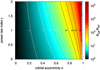 |
Fig. B.1. Colour-coded ratio R0A/R0P of stellar bow-shock sizes between the apocentre and the pericentre of the corresponding orbit in the e − γ plane (see also Eq. (B.8)). The white and black lines correspond to the contours of the constant ratio with numbers indicating the value of R0A/R0P for a given contour. |
where (R0A/R0P)0 is the ratio with a neglected thermal pressure, Eq. (B.8). The thermal term at the pericentre may be evaluated as follows,
 (B.14)
where TP is the gas temperature at the pericentre,  is the mean molecular weight, and mp is a proton mass. The ratio of the thermal terms at the apocentre and the pericentre is then
 (B.15)
where δ ≥ 0 is a power-law index of the spherical temperature profile of the ambient medium, Ta(r) = T0(r0/r)δ, where T0 = Ta(r0). The extra term in Eq. (B.13) would vanish if αP = αA, which would occur if e = 0. Using Eq. (B.15) we may rewrite Eq. (B.13) in the following form,
![Mathematical equation: $$ \begin{aligned} \frac{R_{0A}}{R_{0P}}=\left(\frac{R_{0A}}{R_{0P}}\right)_0 \underbrace{\left[\frac{1+\alpha _{\rm {P}}(T_{\rm {P}},a,e)}{1+\alpha _{\rm {P}}(T_{\rm {P}},a,e)\left(\frac{1+e}{1-e}\right)^{2-\delta }}\right]^{1/2}}_{F_{AP}(T_{\rm {P}},a,e,\delta )}. \end{aligned} $$](/articles/aa/full_html/2020/12/aa37724-20/aa37724-20-eq42.gif) (B.16)
(B.16)
For the estimation of the factor FAP in brackets, which arises because of thermal pressure, we consider the orbital elements of S2 and the following temperature profile of the ambient medium (Psaltis 2012; Broderick et al. 2011),
 (B.17)
where δ = 0.84 and T0 = 9.5 × 10¹⁰ K. After calculation, the correction term is ≃0.8 for S2 star, and so every ratio in Table B.1 should be slightly adjusted, R0A/R0P ≃ 0.8(R0A/R0P)0, if the temperature profile, Eq. (B.17), holds. Including the thermal pressure term, the formula for the density power-law index γ based on the ratio of the apocentre and the pericentre standoff radii changes accordingly,
![Mathematical equation: $$ \begin{aligned} \gamma ^{\prime }_{AP}=2\big [(\log {(R_{0A}/R_{0P})}-\log {F_{AP}})/\log {[(1+e)/(1-e)]}-1\big ]. \end{aligned} $$](/articles/aa/full_html/2020/12/aa37724-20/aa37724-20-eq44.gif) (B.18)
(B.18)
Similarly, using the semi-latus rectum–pericentre ratio R0, 90/R0P, one can derive the slope  modified by the thermal therm FLP in the following way,
![Mathematical equation: $$ \begin{aligned} \gamma ^{\prime }_{LP}=\frac{2 [\log {(R_{0,90}/R_{0P})}-\log {F_{LP}}]+\log {(1+e^2)}}{\log {(1+e)}}-2, \end{aligned} $$](/articles/aa/full_html/2020/12/aa37724-20/aa37724-20-eq46.gif) (B.19)
(B.19)
where the thermal term is expressed by
![Mathematical equation: $$ \begin{aligned} F_{LP}(T_{\mathrm{p}},a,e) = \left[\frac{1+\alpha _{\mathrm{P}}(T_{\mathrm{P}},a,e)}{1+\alpha _{\mathrm{P}}(T_{\mathrm{P}},a,e)\frac{(1+e)^{2-\delta }}{(1-e)^2}}\right]^{1/2}. \end{aligned} $$](/articles/aa/full_html/2020/12/aa37724-20/aa37724-20-eq47.gif) (B.20)
(B.20)
All Tables
L′-band flux and magnitude of S2 and S65 for seven epochs over a 15-year interval from 2004.317 to 2018.307.
Summary of constraints for the ambient density close to the GC at the S2 periapse based on the two extinction limits, 1σ and fractional variability, and analytical bow-shock models for both the ambient shock and the stellar-wind shock thermal emission.
Power-law index γ and the corresponding ratio between the apocentre and the pericentre bow-shock sizes and the thermal emission luminosities calculated for different eccentricities.
All Figures
|
Fig. 1. S2 star and known dusty objects close to its orbit. Left panel: position of S2 and the dusty source G1 close to the pericentre of S2 around 2002. We also show the orbit of the DSO (Dusty S-cluster Object, also known as G2). The points of the sources represent colour-coded radial velocities according to the axis on the right. The grey circle in the bottom left corner represents the diffraction limited FWHM of 98 mas corresponding to NACO L′-band. Right panel: position of S2 and dusty source G1 at the pericentre passage of S2 at 2018.38. The orbital parameters were adopted from Gravity Collaboration (2018a) (S2 star), Valencia-S et al. (2015) (DSO source), and Witzel et al. (2017) (G1 source). |
| In the text | |
|
Fig. 2. NACO L′-band mosaic of the GC in 2013.356. North is up and east is to the left. The identification of three stars (S26, S30 and S35) as photometric calibrators is depicted in particular. The black cross shows the IR counterpart of Sgr A*. In order to check any variability in the flux of S2, we used S65 as a reference star. |
| In the text | |
|
Fig. 3. Light curve of S2 and S65 in L′-band over seven observational epochs. |
| In the text | |
|
Fig. 4. Light curve at the position of S2 and the IR counterpart of Sgr A* and our reference star, S65, in 2018.307 in L′-band. The light curve shows that the IR counterpart of Sgr A* is in quiescence during our observation, and therefore the light curve belongs to S2. |
| In the text | |
|
Fig. 5. Illustrative figure of the motion of S2 through the hot flow around Sgr A* of variable density. The density may change by as much as an order of magnitude from the apocentre to the pericentre, from several hundred particles per cubic centimetre to several thousand particles per cubic centimetre, respectively, depending on the power-law slope of the radial number density distribution. For the exemplary calculation, we used na = nB(r/rB)−1, where nB = 20.3 cm−3 is the particle density at the Bondi radius. The white circle in the bottom left corner depicts the L′-band point spread function corresponding to 8m-class telescopes, from which it is apparent that the S2 bow shock remains unresolved, especially close to the pericentre. |
| In the text | |
|
Fig. 6. Temporal evolution of the number density of the ambient medium for the three different density slopes of the radial density profile, na = n0(r/r0)−γ, where γ is equal to 0.5, 1.0, and 1.5; see the plot legend. The dashed red lines indicate the number densities that were observationally inferred by Baganoff et al. (2003) (26 cm−3 at the Bondi radius) and Gillessen et al. (2019) (4000 cm−3 at ∼1000 rs). |
| In the text | |
|
Fig. 7. Total SED of the S2 star (black solid line) around L′ band. |
| In the text | |
|
Fig. 8. Number density and thickness of the two shock layers in the two-shock approximation model as a function of the distance from Sgr A* (in Schwarzschild radii). Left: number density (expressed in cm−3) of the shock driven into the ambient medium (red lines) and of the shocked stellar wind (blue lines) calculated for three specific values of the ambient density slope: γ = 0.5, 1.0, and 1.5. Right: thickness (expressed in cm) of the stellar-wind (blue lines) and ambient shock layers (red lines) calculated for the three different density slopes as in the left panel. |
| In the text | |
|
Fig. 9. Comparison of model light curves based on the mean S2 emission and the modelled thermal emission of its bow shock (solid green and blue lines) with the observed L′-band emission of S2 (red points with errorbars). Upper panels: modelled thermal emission of the bow shock is associated with the extinction of A = 0.04 mag, which was inferred from the standard deviation of observed light curve points. We model the thermal dust emission of the ambient bow shock (solid green line in left panel) and the thermal emission of the stellar-wind shock (solid blue line in right panel) separately. The horizontal solid black line represents the light curve mean value, while the dashed black lines stand for the standard deviation. Lower panels: as in the upper panels, but for the extinction of A = 0.02 mag based on the excess variance of the observed light-curve points. |
| In the text | |
|
Fig. 10. Non-thermal contribution of the S2 bow shock to its L′-band emission. In the left panel, we plot the L′-band light curve as calculated for the S2 bow-shock synchrotron emission for the peak flux of 0.91 mJy (solid black line) and for the peak flux of 0.22 mJy (dashed black line). For comparison, we also show the fractional variability of S2 (dotted green line) and its maximum flux difference (dot-dashed line). The measured mean flux of Sgr A* in L′-band, 4.33 ± 0.18 mJy, is depicted by a dashed blue line. The sum of the mean flux density of S2 with the maximum potential contribution of the non-thermal bow-shock emission is represented by a solid red line. The measured flux density of S2 from 2018.307 is marked by an orange cross. In the right panel, we show the SED of S2 bow-shock synchrotron emission as calculated for the S2 pericentre for the L′-band flux of 0.91 mJy (solid line) and for the L′-band flux of 0.22 mJy (dashed line). The orange dot-dashed line marks the L′-band frequency range and the red star symbol represents the mean flux density of S2 in L′-band. The blue solid line represents the SED of Sgr A* based on the advection dominated accretion flows (ADAFs; Yuan et al. 2003; Yuan & Narayan 2014). |
| In the text | |
|
Fig. 11. Comparison of the upper density limits that are marked as downward arrows inferred from the L′-band light curve of the S2 star based on modelling ambient and stellar-wind shocks for the dust-extinction values of 0.04 and 0.02 mag with different density profiles and structures according to the plot legend and the description. Alongside the density limit based on the thermal bow-shock emission, we also depict the limit based on the non-thermal bow-shock emission (bluish downward arrows). For comparison, we show the density limit of 26 cm−3 inferred by Baganoff et al. (2003) based on the analysis of the X-ray thermal bremsstrahlung profile. Then we show the density constraint of (5 ± 3) × 103 cm−3 inferred from the potential hydrodynamic drag acting on the DSO/G2 object (Gillessen et al. 2019). The general density power-law profiles are depicted by black lines: the solid line stands for the slope of 1.0, the dashed line represents the flat profile of γ = 0.5, and the dot-dashed line depicts the steeper Bondi-like spherical flow with γ = 1.5. The shaded rectangle shows the distance and the density limits (n ∼ 105 − 106 cm−3) of the putative cool disc whose discovery is claimed by Murchikova et al. (2019). The black-framed rectangle depicts the typical densities of the broad-line region (BLR) clouds in the range of n ∼ 108 − 1011 cm−3. The gray lines depict the number density values expected for a thin disc (Shakura & Sunyaev 1973) for the accretion rate of Ṁ = 10−9 − 10−7 M⊙ yr−1 and the viscosity parameter of α = 0.1. The brown-shaded area to the lower left shows the set of density profiles determined using the rotation measure of the submillimeter polarisation measurements (Marrone et al. 2006, 2007) for the inner radii of rin = 300 rs and rin = 3 rs, density slopes of γ = 0.5−1.5, and the accretion rates in the range 2 × 10⁻⁹ − 2 × 10⁻⁷ M⊙ yr−1. The blue dot-dashed vertical at 100 rs and the blue dot-dashed arrow to the left denote the region of a potential magnetically arrested flow (MAD), where the accretion flow changes from continuous to clumpy due to the accumulated poloidal magnetic flux (see e.g. Narayan et al. 2003; Tursunov et al. 2020). The dotted vertical lines mark the periapsis of the S62 star at ∼225 rs and the periapsis of the S2 star at ∼1512 rs. Next to the S2 pericentre vertical line, we highlight the range of densities potentially being explored using L′-band METIS at ELT imaging mode. |
| In the text | |
|
Fig. B.1. Colour-coded ratio R0A/R0P of stellar bow-shock sizes between the apocentre and the pericentre of the corresponding orbit in the e − γ plane (see also Eq. (B.8)). The white and black lines correspond to the contours of the constant ratio with numbers indicating the value of R0A/R0P for a given contour. |
| In the text | |
Current usage metrics show cumulative count of Article Views (full-text article views including HTML views, PDF and ePub downloads, according to the available data) and Abstracts Views on Vision4Press platform.
Data correspond to usage on the plateform after 2015. The current usage metrics is available 48-96 hours after online publication and is updated daily on week days.
Initial download of the metrics may take a while.