© ESO 2020

1. Introduction

Magnetic helicity is a general measure of the complexity of magnetic fields that concisely expresses the amount of twist, writhe, and mutual winding of field lines in a given configuration (Elsasser 1956; Berger 1999). When applied to magnetized plasmas, the concept of helicity acquires the very special role of an integral of motion. Intuitively, this is because, as Alfvén’s theorem demonstrates, in ideal magneto-hydrodynamics the topology of the magnetic field cannot be changed by plasma motions. As ideal evolution cannot change the field topology, and therefore the entanglement of the field lines, magnetic helicity is conserved in dissipationless (ideal) plasmas (Woltjer 1958), and is almost conserved in mildly collisional ones (Matthaeus & Goldstein 1982; Berger 1984). From a different perspective, the inverse cascade that characterizes magnetic helicity (see, e.g., Frisch et al. 1975; Alexakis et al. 2006; Müller & Malapaka 2013), as opposed to the direct cascade of magnetic energy towards the small dissipative scales, is often invoked as the underlying paradigm behind the appearance of large-scale magnetic fields (see, e.g., Antiochos 2013). Taken together, the conservation and inverse-cascade properties give magnetic helicity the unique potential to describe the evolution of magnetized plasma.

The concept of magnetic helicity is very general, and the wide applicability of magneto-hydrodynamics makes helicity a cross-disciplinary tool. In the solar context, for instance, it was applied to topics such as dynamos (Brandenburg & Subramanian 2005), reconnection (Del Sordo et al. 2010), fluxes of helicity through the photosphere (Pariat et al. 2005; Démoulin & Pariat 2009; Schuck & Antiochos 2019), the distribution of helicity in the corona (Yeates & Hornig 2016), the initiation of coronal mass ejections (CMEs; Pariat et al. 2017; Thalmann et al. 2019) and their link to interplanetary CMEs (Nakwacki et al. 2011; Temmer et al. 2017), just to name a few examples. All these type of studies are related to each other in that they treat different aspects of the generation and evolution of the solar magnetic field that are constrained by the conservation of magnetic helicity.

Magnetic helicity is expressed as the volume integral of the magnetic field and its vector potential (see Eq. (1) below), and is therefore gauge-dependent, unless the considered volume is bounded by a magnetic flux surface. Such a requirement is generally not satisfied by natural plasmas, nor in numerical simulations. In order to overcome this limitation, Berger & Field (1984) and Finn & Antonsen (1985) introduced the concept of relative magnetic helicity, where the helicity in an arbitrarily shaped finite volume is computed with respect to a reference field that has specific properties at the boundary. In this way, the values obtained by the volume integral are made independent from the details used in the vector potential computation, that is, they are gauge-invariant.

Insofar as the different processes involved can be described by magneto-hydrodynamics, the helicity of the field generated in the interior of the Sun must be conserved during the buoyant phase, through its rearrangement during the emergence through the photospheric layer forming long-lived coronal structures that finally erupt (see e.g., Priest et al. 2016), to its propagation through interplanetary space (e.g., Démoulin et al. 2002; Green 2002; Nindos et al. 2003; Thalmann et al. 2019). In principle, a budget of (relative) magnetic helicity can be built that accounts for the transformation of the magnetic field from the interior of the Sun up to transient perturbations of interplanetary CMEs (e.g., Berger & Ruzmaikin 2000; Démoulin et al. 2016). To exploit such a remarkable property requires the quantitative separation and comparison of, for example, the helicity emerging in the corona and the helicity left under the photosphere; or the helicity ejected as a CME (and probed at the spacecraft position) and that left behind on the Sun.

Numerical simulations of different degrees of realism are available for all those processes. However, there is a principal difficulty in separating the helicity into subvolume contributions: a limited number of very specific applications (Berger & Field 1984; Longcope & Malanushenko 2008) have shown that the sum of the relative helicity in two contiguous subvolumes is not simply equal to the helicity of the total volume. In this sense, relative magnetic helicity is not an algebraically additive quantity. This is a serious impediment to the exploitation of the conservation principle in building global budgets of relative magnetic helicity. In addition, the discussion of the additivity issue by Berger & Field (1984) applies to volumes that are either unbounded or bounded by a flux surface, which are conditions that are not normally satisfied in numerical simulations. Similarly, Longcope & Malanushenko (2008) proposes an extension of the formalism in Berger & Field (1984) that is intended to be applied to the finite volumes of numerical simulations, but still considers a coronal volume that is bounded above by a flux surface. Finally, the choice of gauge made in Berger & Field (1984) and Longcope & Malanushenko (2008) is only one of the possibilities for discussing the nonadditivity property, and may not be always available to specific applications where the gauge choice is limited by other factors (e.g., by numerical precision).

The main goal of this work is to derive general equations for the additivity of the relative magnetic helicity in finite volumes, and to provide a gauge-invariant expression for the nonadditive terms. In particular, the additivity problem is formulated here as a partition problem between two subvolumes that are contiguous and share a common boundary, such as for example in the flux emergence process where helicity is transferred from a sub-photospheric volume to the coronal volume. The generality of our treatment is such that, on the one hand, it allows us to identify the reason for the nonadditivity in a general way. On the other hand, our method can be easily adapted to different geometries and gauge choices, allowing for straightforward applications to numerical simulations.

In Sect. 2 we discuss the nature of the additivity problem; we then derive the general partition equation without any assumptions on either the shape of the volumes and interface, or the employed gauge. Section 3 gives a brief overview of how the partition equation is modified by the choice of commonly used gauges, which are then applied in Sect. 4 to derive known expressions for the partition formula that are used in the literature. A numerical application to a solution of the force-free equation is used in Sect. 5 to verify the accuracy of the partition formula and to test the importance of the nonadditive term with respect to the helicity of the field. Finally, in Sect. 6 we summarize our results, discuss their implication for the definition of the relative magnetic helicity, and propose a number of applications of our formalism.

2. Partition of helicity between two volumes

2.1. General definitions

As usual, for a magnetic field B and its associated vector potential A, we define the gauge-dependent magnetic helicity ℋ in a volume 𝒱 as

$$\begin{array}{c}\hfill \mathcal{H}(\mathit{B},\mathcal{V})={\displaystyle {\int }_{\mathcal{V}}}\mathit{A}·\mathit{B}\mathrm{d}\mathcal{V},\end{array}$$(1)

and the gauge-invariant relative magnetic helicity (Finn & Antonsen 1985) as

$$\begin{array}{c}\hfill H(\mathit{B},\mathcal{V})={\displaystyle {\int }_{\mathcal{V}}}(\mathit{A}+{\mathit{A}}_p)·(\mathit{B}-{\mathit{B}}_p)\mathrm{d}\mathcal{V},\end{array}$$(2)

where the field B_p of vector potential A_p satisfies

$$\begin{array}{c}\hfill {\widehat{\mathit{n}}·{\mathit{B}}_p|}_{\partial \mathcal{V}}={\widehat{\mathit{n}}·\mathit{B}|}_{\partial \mathcal{V}}\end{array}$$(3)

on the boundary ∂𝒱, with $\widehat{\mathit{n}}$ the external normal to ∂𝒱. By construction, ∂𝒱 is a flux surface for the field B_j  =  B − B_p. Any reference field that satisfies Eq. (3), and the solenoidal condition ∇ ⋅ B_p  =  0, ensures the gauge-invariance of Eq. (2). In this work we assume that all magnetic fields satisfy the solenoidal condition exactly. A discussion of the consequences of the violation of the solenoidal condition in numerical computation of helicity and energy can be found in Valori et al. (2016) and Valori et al. (2013), respectively.

In principle, any field that satisfies Eq. (3) can be used as reference field, with Eq. (2) defining the helicity relative to the chosen reference field. We adopt the common choice of a potential field as reference field B_p. In this case, B_p is written as a function of the scalar potential ϕ as B_p  =  ∇ϕ, where ϕ satisfies the Laplace equation Δϕ  =  0 in 𝒱 with the Neumann boundary condition

$$\begin{array}{c}\hfill {\widehat{\mathit{n}}·\mathbf{\nabla }\varphi |}_{\partial \mathcal{V}}={\widehat{\mathit{n}}·\mathit{B}|}_{\partial \mathcal{V}},\\ \hfill \end{array}$$(4)

such that the gauge-invariance requirement Eq. (3) is satisfied. Equation (4) uniquely defines B_p in 𝒱, and defines ϕ in 𝒱 up to an additive constant. The potential field defined by Eq. (4) has the minimal energy for the given distribution of the normal component of the field on the boundary, ${\widehat{\mathit{n}}·\mathit{B}|}_{\partial \mathcal{V}}$, see for example Valori et al. (2013). Therefore, this customary choice is not only convenient in its simplicity, but carries also a deeper physical meaning of the potential field being the “ground state” for a given distribution of field on the boundary, especially within the magneto-hydrodynamical framework; see for example Schuck & Antiochos (2019). Moreover, if B_p is the potential field in 𝒱, then B_j is the part of the magnetic field that is related to the presence of currents in 𝒱, sometimes referred to as the current-carrying part of the field. We adopt the potential field as defined above as reference field in the remainder of the article, but we explicitly discuss the consequences of this choice on our results, when relevant.

The relative magnetic helicity, Eq. (2), can be recast as the sum of three nongauge-invariant terms:

$$\begin{array}{c}\hfill H(\mathit{B},\mathcal{V})=\mathcal{H}(\mathit{B},\mathcal{V})-\mathcal{H}({\mathit{B}}_p,\mathcal{V})+{\mathcal{H}}_{\mathrm{mix}}(\mathit{B},{\mathit{B}}_p,\mathcal{V}),\end{array}$$(5)

which is the difference between the magnetic helicity of B and B_p plus a “mixed term” defined as

$$\begin{array}{cc}& {\mathcal{H}}_{\mathrm{mix}}(\mathit{B},{\mathit{B}}_p,\mathcal{V})={\displaystyle {\int }_{\mathcal{V}}}({\mathit{A}}_p·\mathit{B}-\mathit{A}·{\mathit{B}}_p)\mathrm{d}\mathcal{V}\hfill \\ \hfill & ={\displaystyle {\int }_{\partial \mathcal{V}}}(\mathit{A}\times {\mathit{A}}_p)·\mathrm{d}\mathit{S},\hfill \end{array}$$(6)

where $\text{d}\mathit{S}=\widehat{\mathit{n}}\text{d}S$ is the oriented infinitesimal surface element on ∂𝒱.

2.2. Volume partition

We consider the case of two contiguous volumes of finite size and 𝒱 = 𝒱^a ∪ 𝒱^b, such that 𝒱^a and 𝒱^b are bounded by the surfaces ∂𝒱^a and ∂𝒱^b with external normals ${\widehat{\mathit{n}}}^a$ and ${\widehat{\mathit{n}}}^b$, respectively. Figure 1 shows a graphical representation of the volumes involved. The boundary surface of each subvolume can be split into an interface (Σ) plus a noninterface (Ʒ) contribution as

$$\partial {\mathcal{V}}^a={\mathrm{\Sigma }}^a\cup {\mathrm{Ʒ}}^a,$$(7)

$$\partial {\mathcal{V}}^b={\mathrm{\Sigma }}^b\cup {\mathrm{Ʒ}}^b,$$(8)

with the boundary ∂𝒱 of the volume 𝒱 given

by

$$\begin{array}{c}\hfill \partial \mathcal{V}={\mathrm{Ʒ}}^a\cup {\mathrm{Ʒ}}^b.\end{array}$$(9)

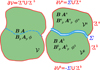Fig. 1. Sketch of the volume splitting: an interface Σ splits the finite volume 𝒱 bounded by ∂𝒱 into two subdomains, 𝒱a and 𝒱b, each one bounded by the surface ∂𝒱a and ∂𝒱b, respectively.

The interfaces Σ^a and Σ^b represent the same surface but differ for the orientation of the normal, ${\widehat{\mathit{n}}}^a=-{\widehat{\mathit{n}}}^b$. When the orientation of the normal is not required, we drop the superscript from Σ. In order to have a more compact notation, we also introduce

$$\begin{array}{c}\hfill Z^{\mathit{ab}}=\{\begin{array}{cc}{Z}^a\hfill & \forall \mathit{x}\in {\mathcal{V}}^a\hfill \\ Z^b\hfill & \forall \mathit{x}\in {\mathcal{V}}^b,\hfill \end{array}\end{array}$$(10)

where Z is any function or vector defined separately in 𝒱^a and 𝒱^b.

All volumes are assumed to be simply connected in order to avoid the difficulties of multi-valued gauge functions, but no assumption is made on the shape of the volumes or of the interface. No further assumption is made at this point about the geometry of the system.

For each of the three considered volumes 𝒱, 𝒱^a, and 𝒱^b, the relative magnetic helicity, Eq. (2), can be computed. The question that we wish to address in this section is: what is the general relation between the three correspondent relative helicity values H(B, 𝒱), H(B, 𝒱^a), and H(B, 𝒱^b)?

2.3. Difference in the reference fields

The relative helicity Eq. (2) is gauge-invariant because the reference potential field B_p for the full volume 𝒱 is defined by Eq. (4), thus satisfying the gauge-invariance condition Eq. (3). Similarly, the computation of the relative helicity for the two subvolumes 𝒱^a and 𝒱^b requires that reference fields be defined such that they fulfil the same condition, Eq. (3), but in each subvolume separately. In other words, the (potential) reference fields ${\mathit{B}}_p^a$ and ${\mathit{B}}_p^b$ are uniquely defined by Δϕ^a = 0 in 𝒱^a and the boundary condition

$$\begin{array}{c}\hfill {{\widehat{\mathit{n}}}^a·\mathbf{\nabla }{\varphi }^a|}_{\partial {\mathcal{V}}^a}={{\widehat{\mathit{n}}}^a·\mathit{B}|}_{\partial {\mathcal{V}}^a},\\ \hfill \end{array}$$(11)

and Δϕ^b = 0 in 𝒱^b and the boundary condition

$$\begin{array}{c}\hfill {{\widehat{\mathit{n}}}^b·\mathbf{\nabla }{\varphi }^b|}_{\partial {\mathcal{V}}^b}={{\widehat{\mathit{n}}}^b·\mathit{B}|}_{\partial {\mathcal{V}}^b},\end{array}$$(12)

respectively. We note that, because of the way the volume 𝒱 is split, the boundary conditions for the above Laplacian equations on the noninterface boundaries Ʒ^ab of 𝒱^a and 𝒱^b are the same as for B_p (see Fig. 1).

In order to understand the differences between the reference fields, let us first consider a special case: if $\widehat{\mathit{n}}·\mathit{B}=\widehat{\mathit{n}}·{\mathit{B}}_p$ on the interface Σ, then the normal components of ${\mathit{B}}_p^a$ and ${\mathit{B}}_p^b$ also match that of B_p on the interface Σ. It then follows from the uniqueness of the solution to the Laplace problems that, in this special case, it is ${\mathit{B}}_p^a$ = B_p in 𝒱^a and ${\mathit{B}}_p^b$ = B_p in 𝒱^b. The combined field ${\mathit{B}}_p^{\mathrm{ab}}$ as defined by Eq. (10) is continuous across Σ, and we have ${\mathit{B}}_p^{\mathrm{ab}}={\mathit{B}}_p$.

However, for a generic B field, $\widehat{\mathit{n}}·\mathit{B}$ is different from $\widehat{\mathit{n}}·{\mathit{B}}_p$ on the interface Σ. Therefore, in the general case, the solutions of the Laplacian equations in 𝒱^a and 𝒱^b provide potential fields ${\mathit{B}}_p^a$ and ${\mathit{B}}_p^b$ that are different from B_p in each of the subvolumes. Moreover, the transverse components of ${\mathit{B}}_p^a$ and ${\mathit{B}}_p^b$ are in general different on both sides of the interface Σ. The corresponding field ${\mathit{B}}_p^{\mathrm{ab}}$ in the full volume 𝒱 is not fully potential but it contains a current sheet on Σ. As we show in the following section, this difference between the reference field in 𝒱 and in the subvolumes 𝒱^a and 𝒱^b is at the core of the nonadditivity of relative magnetic helicity.

It is worth noting that the difference between B_p and ${\mathit{B}}_p^a$ (respectively, ${\mathit{B}}_p^b$) in 𝒱^a (respectively, 𝒱^b) is not a consequence of the choice of potential fields as reference fields. Indeed, the same difference is to be expected for other nonpotential reference fields. This is because, on the one hand, the gauge-invariance condition Eq. (3) needs to be imposed on the interface Σ for the reference fields of 𝒱^a and of 𝒱^b. On the other hand, Σ is not a boundary of 𝒱, and therefore the reference field of 𝒱 cannot be specified on Σ. We conclude that, in general, the reference field B_p in 𝒱 is not derived from the same information as ${\mathit{B}}_p^a$ and ${\mathit{B}}_p^b$, and therefore B_p is not simply the juxtaposition of the reference fields ${\mathit{B}}_p^a$ in 𝒱^a and ${\mathit{B}}_p^b$ in 𝒱^b. This, and the resulting discontinuity between ${\mathit{B}}_p^a$ and ${\mathit{B}}_p^b$ across Σ discussed above, are direct consequences of the property of Eq. (3) that reference fields must fulfil in order for the relative magnetic helicity (Eq. (2)) to be gauge-invariant.

Before we consider the relative helicity, let us first briefly discuss the consequences of the volume splitting on the magnetic energy

$$\begin{array}{c}\hfill \mathcal{E}(\mathit{B},\mathcal{V})=\frac{1}{2{\mu }_0}{\displaystyle {\int }_{\mathcal{V}}}{B}^2\mathrm{d}\mathcal{V},\end{array}$$(13)

and the relative (or free) magnetic energy

$$\begin{array}{c}\hfill E(\mathit{B},\mathcal{V})=\frac{1}{2{\mu }_0}{\displaystyle {\int }_{\mathcal{V}}}(B^2-B_p^2)\mathrm{d}\mathcal{V}.\end{array}$$(14)

By introducing the volume splitting of Sect. 2.2 to the free energy, we have

$$\begin{array}{c}\hfill E(\mathit{B},\mathcal{V})-E(\mathit{B},{\mathcal{V}}^a)-E(\mathit{B},{\mathcal{V}}^b)=\frac{1}{2{\mu }_0}{\displaystyle {\int }_{\mathcal{V}}}({(B_p^{\mathit{ab}})}^2-B_p^2)\mathrm{d}\mathcal{V}.\end{array}$$(15)

As the right-hand side of Eq. (15) is, in general, nonvanishing, then the free energy in 𝒱 is not simply equal to the sum of the free energies in the composing subvolumes 𝒱^a and 𝒱^b, that is the free energy is a nonadditive quantity. In particular, the difference between the reference magnetic fields in 𝒱^a and 𝒱^b and the one in 𝒱 implies the nonadditivity of the relative energy, while the energy ℰ is manifestly additive.

2.4. Relative magnetic helicity of contiguous volumes: general formulation

Without loss of generality, the relative magnetic helicity in 𝒱 can be formally written as

$$\begin{array}{c}\hfill H(\mathit{B},\mathcal{V})=H(\mathit{B},{\mathcal{V}}^a)+H(\mathit{B},{\mathcal{V}}^b)+\delta H,\end{array}$$(16)

with

$$\begin{array}{cc}& \delta H=H(\mathit{B},\mathcal{V})-H(\mathit{B},{\mathcal{V}}^a)-H(\mathit{B},{\mathcal{V}}^b)\hfill \\ \hfill & =\delta \mathcal{H}-\delta {\mathcal{H}}_p+\delta {\mathcal{H}}_{\mathrm{mix}},\hfill \end{array}$$(17)

where we defined

$$\delta \mathcal{H}=\mathcal{H}(\mathit{B},\mathcal{V})-\mathcal{H}(\mathit{B},{\mathcal{V}}^a)-\mathcal{H}(\mathit{B},{\mathcal{V}}^b)$$(18)

$$\delta {\mathcal{H}}_p=\mathcal{H}({\mathit{B}}_p,\mathcal{V})-\mathcal{H}({\mathit{B}}_p^a,{\mathcal{V}}^a)-\mathcal{H}({\mathit{B}}_p^b,{\mathcal{V}}^b)$$(19)

$$\begin{array}{cc}\hfill & \delta {\mathcal{H}}_{\mathrm{mix}}={\mathcal{H}}_{\mathrm{mix}}(\mathit{B},{\mathit{B}}_p,\mathcal{V})-{\mathcal{H}}_{\mathrm{mix}}(\mathit{B},{\mathit{B}}_p^a,{\mathcal{V}}^a)\hfill \\ \hfill & -{\mathcal{H}}_{\mathrm{mix}}(\mathit{B},{\mathit{B}}_p^b,{\mathcal{V}}^b).\hfill \end{array}$$(20)

Equation (16) is the result of a simple reorganization that collects in δH all contributions that make the relative magnetic helicity a nonadditive quantity and, by grouping similar terms together, allows for cancelations between them. In Appendix A, we show that by using Eqs. (1) and (6) in Eq. (17), we obtain

$$\begin{array}{c}\hfill \delta \mathcal{H}={\displaystyle {\int }_{\mathrm{\Sigma }}}\chi (\mathit{B}·\mathrm{d}{\mathit{S}}^a),\end{array}$$(21)

$$\begin{array}{c}\hfill \delta {\mathcal{H}}_p=\delta {\mathcal{H}}_p^{\mathrm{Coul}}+\delta {\mathcal{H}}_p^{\mathrm{Surf}}\end{array}$$(22)

where

$$\begin{array}{cc}& \delta {\mathcal{H}}_p^{\mathrm{Coul}}={\displaystyle {\int }_{{\mathcal{V}}^a}}{\varphi }^a(\mathbf{\nabla }·{\mathit{A}}_p^a)\mathrm{d}\mathcal{V}+{\displaystyle {\int }_{{\mathcal{V}}^b}}{\varphi }^b(\mathbf{\nabla }·{\mathit{A}}_p^b)\mathrm{d}\mathcal{V}\hfill \\ \hfill & -{\displaystyle {\int }_{\mathcal{V}}}\varphi (\mathbf{\nabla }·{\mathit{A}}_p)\mathrm{d}\mathcal{V},\hfill \end{array}$$(23)

$$\begin{array}{cc}\hfill & \delta {\mathcal{H}}_p^{\mathrm{Surf}}={\displaystyle {\int }_{\partial \mathcal{V}}}(\varphi {\mathit{A}}_p-{\varphi }^{\mathit{ab}}{\mathit{A}}_p^{\mathit{ab}})·\mathrm{d}\mathit{S}\hfill \\ \hfill & -{\displaystyle {\int }_{\mathrm{\Sigma }}}({\varphi }^a{\mathit{A}}_p^a-{\varphi }^b{\mathit{A}}_p^b)·\mathrm{d}{\mathit{S}}^a,\hfill \end{array}$$(24)

and

$$\begin{array}{cc}& \delta {\mathcal{H}}_{\mathrm{mix}}={\displaystyle {\int }_{\partial \mathcal{V}}}({\mathit{A}}^{\mathit{ab}}\times ({\mathit{A}}_p-{\mathit{A}}_p^{\mathit{ab}}))·\mathrm{d}\mathit{S}\hfill \\ \hfill & +{\displaystyle {\int }_{\mathrm{\Sigma }}}[{\mathit{A}}^a\times ({\mathit{A}}_p-{\mathit{A}}_p^a)-{\mathit{A}}^b\times ({\mathit{A}}_p-{\mathit{A}}_p^b)]·\mathrm{d}{\mathit{S}}^a\hfill \\ \hfill & -{\displaystyle {\int }_{\mathrm{\Sigma }}}\chi ({\mathit{B}}_p·\mathrm{d}{\mathit{S}}^a),\hfill \end{array}$$(25)

where we use the notation of Eq. (10) for all fields defined in the subvolumes 𝒱^a and 𝒱^b, and χ is the gauge function defined by

$$\begin{array}{c}\hfill \mathbf{\nabla }\chi ={({\mathit{A}}^b-{\mathit{A}}^a)|}_{\mathrm{\Sigma }},\end{array}$$(26)

with χ a function of the interface variables only; see Eq. (A.22). On the interface Σ, the infinitesimal oriented surface was chosen to be that of dS^a. The study of the properties of Eqs. (16)–(25) is the main focus of this article.

The first and most important result is that Eq. (16) shows in the most general way that the relative magnetic helicity is not an algebraically additive quantity: The relative magnetic helicity in the entire volume 𝒱 is not simply the sum of the relative helicity of the composing subvolumes 𝒱^a and 𝒱^b, but a general non-vanishing additional term, δH, is present. We note that, because the left-hand side (LHS) and the first two terms on the right-hand side (RHS) of Eq. (16) are gauge-invariant, then δH must be globally gauge-invariant too. Appendix B outlines how to see this directly from the terms in δH.

The gauge-invariance of Eq. (16) implies that the nonadditivity of relative magnetic helicity is a general property: a special gauge that makes the relative helicity additive (or even partitionable between volumes) does not exist. This does not rule out that a very special combination of geometry, choice of reference field, and boundary conditions may exist in which relative magnetic helicity is additive, but this is not true in general.

Finally, we note that Eqs. (21)–(25) contain three types of terms in the representation that we have chosen, namely volume, interface, and outer boundaries (or noninterface) surface terms. This formalism allows for a more direct treatment of specific limits in the following sections, but is by no means the only possible one. Let us now discuss the individual nonadditivity terms.

2.4.1. δℋ : Nonadditivity of the magnetic helicity

The nonadditive term δℋ of Eq. (21) is an interface term that, for arbitrary B, depends solely on the gauge specification, and can therefore be eliminated by specific gauge choices for A^a and A^b that insure χ = 0 on Σ; see Sect. 3.4.

2.4.2. δℋ_p : Nonadditivity of the helicity of the reference fields

The δℋ_p in Eq. (22) is composed of a volume and surface terms. The volume term, $\delta {\mathcal{H}}_p^{\mathrm{Coul}}$ contains the Coulomb gauge conditions for the three reference fields, a gauge that can be chosen to have this term vanish. It is interesting to note that the Coulomb conditions appear explicitly only in relation to reference fields, and not for any of the other vector potentials. The same happens for the time evolution of the relative magnetic helicity in Eq. (25) of Pariat et al. (2015a), and in Eqs. (13), (41) regulating the evolution of the current-carrying and volume-threading relative magnetic helicity derived by Linan et al. (2018). All these cases express helicity contributions due to sources in the vector potentials of the potential fields, and thereby in the helicity of the reference potential fields.

While $\delta {\mathcal{H}}_p^{\mathrm{Coul}}$ accounts for volume differences, the surface term $\delta {\mathcal{H}}_p^{\mathrm{Surf}}$ in Eq. (24) contains interface and noninterface contributions that depend on the components of the vector potentials of the reference fields that are normal to the boundaries, and on the scalar potentials of the same reference fields. Since the reference fields in 𝒱 and 𝒱^a (𝒱 and 𝒱^b, respectively) do not represent the same field (see Sect. 2.3), there is no general gauge relation between the vector potentials A_p and ${\mathit{A}}_p^a$ (A_p and ${\mathit{A}}_p^b$, respectively) that can be used to simplify these expressions.

The last term in Eq. (24) is an interface term accounting for the discontinuity of the transverse components in the reference fields at Σ. As discussed in Sect. 2.3, this term can be seen as the contribution due to a surface current generated by the discontinuity of the transverse components of ${\mathit{B}}_p^a$ and ${\mathit{B}}_p^b$ across Σ; see also Sect. 4.1.

2.4.3. δℋ_mix: Nonadditivity of the mixed helicity

The first two integrals in Eq. (25) are directly related to the transverse components of the vector potentials at the boundaries. The additional complication of Eq. (25) with respect to the simpler Eq. (6) is that such integrals involve cross interactions between different vector potentials.

The last term in Eq. (25) is similar to that in δℋ, but involves B_p rather than B, and similar considerations hold. Since, in general, B and B_p differ on Σ, then the combination of these two terms is nonzero, and is related to the current-carrying part of the field, B_j. Unless the gauge choices for A^a and A^b ensure χ = 0, the only other case where the two terms cancel each other is when B = B_p on Σ, which, according to the discussion in Sect. 2.3, is a very special case.

In summary, the nonadditivity of the relative helicity H has the same origin as that of the relative energy E, a difference of reference field in each subvolume with the one in the full volume. This is the case even when the lowest energy state, the potential field, is selected as reference field. Still, the nonadditivity terms of H are much more complex than the one for E, as they also involve the vector potentials.

3. Applications of the partition equation with specific gauges

Equation (16) is a gauge-invariant, general expression of the relative helicity partition that does not make any assumption about the specific gauges and boundary conditions that are used to compute the vector potentials. Such specifications are however required for its practical application.

The constraints on the scalar and vector potentials defined so far derive from the gauge-invariance constraint; see Eq. (3) and Sect. 2.3. In particular, the scalar potentials are determined by solving the Poisson problems Eqs. (A.8) and (A.9) that define ϕ, ϕ^a, and ϕ^b each modulo a constant. The vector potentials must obey the curl relations with the fields; Eq. (A.2). In addition, the connection between vector potentials of different volumes is prescribed by Eq. (26) (or, more specifically, Eq. (A.22)). This set of constraints is not sufficient to determine the vector potentials.

A gauge should be properly defined as the set of equations and boundary conditions that uniquely determines the scalar and vector potentials for a given magnetic field B in 𝒱. In this sense, in Sect. 5 we refer to different sets of boundary conditions for the vector potentials as different gauges. In a more relaxed sense, we often use the term gauge to mean a group of gauges, such as when we refer to the “Coulomb gauge”, meaning the ∇ ⋅ A = 0 condition only; this is rather a family of gauges, to which additional boundary conditions must be added to uniquely determine the vector potentials.

On the condition that they do not conflict with the other gauge constraints, such additional equations and/or boundary conditions are arbitrary, and thanks to gauge invariance they do not affect the outcome of Eq. (16).

3.1. Coulomb gauge

Assuming that all three vector potentials are solenoidal, $\mathbf{\nabla }\cdot {\mathit{A}}_p=\mathbf{\nabla }\cdot {\mathit{A}}_p^a=\mathrm{\nabla }\cdot {\mathit{A}}_p^b=0$, then $\delta {\mathcal{H}}_p^{\mathrm{Coul}}=0$. In addition, Eq. (A.3) in conjunction with the Coulomb gauge, restricts the possible choice of the gauge functions to the class of functions that satisfy Δχ^a = Δχ^b = 0.

3.2. DeVore-Coulomb gauge

The DeVore gauge (DeVore 2000; Valori et al. 2012; Moraitis et al. 2018) sets one of the components of the vector potential equal to zero. For absolute clarity, let us assume that Σ is a plane parallel to the xy-plane, and set A_z = 0, as in Valori et al. (2012). The main advantage of the DeVore gauge is that it is very accurate and fast to compute numerically (Valori et al. 2016) because the vector potentials are computed by one-dimensional vertical integration of the magnetic field starting from one of the boundaries. A particularly useful formulation of the DeVore gauge requires, in addition, that the two-dimensional integration functions appearing in the computation of the vector potential of the potential field are solenoidal (see Sect. 5 in Valori et al. 2012). In this case, the DeVore gauge ensures that ∇ ⋅ A_p = 0, that is, it is a DeVore-Coulomb gauge for the vector potential. If the DeVore-Coulomb gauge is adopted for all three vector potentials A_p, ${\mathit{A}}_p^a$, and ${\mathit{A}}_p^b$, then also in this case $\delta {\mathcal{H}}_p^{\mathrm{Coul}}=0$.

3.3. Boundary conditions

Before further analyzing Eq. (16), let us first consider the relative magnetic helicity in a single volume as given in Eq. (5). A commonly used condition that is often used in combination with the Coulomb gauge for A_p (see e.g., Berger 1999; Thalmann et al. 2011) is that

$$\begin{array}{c}\hfill \widehat{\mathit{n}}\times \mathit{A}=\widehat{\mathit{n}}\times {\mathit{A}}_p;\end{array}$$(27)

in other words, the vector potential of field and reference field have the same tangential components on the boundary of the considered volume. Such a boundary condition is allowed because Eq. (27) implies Eq. (3). In this case, ℋ_mix(B, B_p, 𝒱) vanishes by Eq. (6) and the relative magnetic helicity of Eq. (2) is equal to the difference between the helicity of the field and the helicity of the relative reference field, that is,

$$\begin{array}{c}\hfill H(\mathit{B},\mathcal{V})=\mathcal{H}(\mathit{B},\mathcal{V})-\mathcal{H}({\mathit{B}}_p,\mathcal{V}),\end{array}$$(28)

which is the definition of relative helicity predating Eq. (2), used for example in Berger (1984) and Jensen & Chu (1984). In the practical computation of vector potentials, Eq. (27) is often indirectly imposed by assuming that A = A_p on ∂𝒱 as a boundary condition for A. However, we stress that the boundary condition in Eq. (27) is not compatible with the DeVore gauge, as shown by Eq. (31) of Valori et al. (2012). Similarly, it is not possible, in general, to have δℋ_mix = 0 in Eq. (25) in this gauge.

A special boundary condition is when ∂𝒱 is a flux surface. In this case, from $\widehat{\mathit{n}}·\mathit{B}=0$, it follows that A can be written as $\mathit{A}=\widehat{\mathit{n}}{A}_n+{\mathbf{\nabla }}_{\perp }\chi$ for some function χ, where ∇_⊥ is the gradient normal to $\widehat{\mathit{n}}$. Then, substituting in Eq. (6), we can extend the ∇_⊥χ to a full gradient without changing the integral, and we obtain

$$\begin{array}{c}\hfill {\mathcal{H}}_{\mathrm{mix}}={\displaystyle {\int }_{\partial \mathcal{V}}}\mathbf{\nabla }\times (\chi {\mathit{A}}_p)·\mathrm{d}\mathit{S}-{\displaystyle {\int }_{\partial \mathcal{V}}}\chi {\mathit{B}}_p·\mathrm{d}\mathit{S},\end{array}$$(29)

where the last term ion the RHS vanishes since, from Eq. (3), ∂𝒱 is also a flux surface of B_p. If the flux surface ∂𝒱 is closed, then the first term on the RHS of Eq. (29) vanishes too, and ℋ_mix = 0 in this case. Moreover, since $\widehat{\mathit{n}}·\mathit{B}=0$ in Eq. (4), then B_p = 0, and H(B, 𝒱) = ℋ(B, 𝒱).

If the boundary condition of Eq. (27) is used in the computation of the three pairs of vector potentials (A, A_p), (A^a, ${\mathit{A}}_p^a$), and (A^b, ${\mathit{A}}_p^b$), then Eq. (20), with Eq. (6) defining ℋ_mix, directly shows that

$$\begin{array}{c}\hfill {\mathcal{H}}_{\mathrm{mix}}(\mathit{B},{\mathit{B}}_p,\mathcal{V})={\mathcal{H}}_{\mathrm{mix}}^a(\mathit{B},{\mathit{B}}_p^a,{\mathcal{V}}^a)={\mathcal{H}}_{\mathrm{mix}}^b(\mathit{B},{\mathit{B}}_p^b,{\mathcal{V}}^b)=0,\end{array}$$(30)

and thus δℋ_mix = 0. The same result can also be obtained directly from Eq. (25) using Eq. (A.3) to write $\widehat{\mathit{n}}\times ({\mathit{A}}_p^{\mathit{ab}}+\mathbf{\nabla }\chi )=\widehat{\mathit{n}}\times {\mathit{A}}_p$.

3.4. Computation of the gauge function χ

The gauge function χ defined by Eq. (26) and appearing in Eqs. (21) and (25) can be computed by direct integration using the fundamental theorem of calculus for line integrals as

$$\begin{array}{c}\hfill \chi (\mathit{x})=\chi (\mathit{a})+{\displaystyle {\int }_{\mathcal{C}(\mathit{a},\mathit{x})}}({\mathit{A}}^b-{\mathit{A}}^a)·\mathrm{d}\mathit{l},\end{array}$$(31)

for any curve 𝒞(a, x) on Σ connecting points a to x, with χ(a) = 0 as a general prescription.

In general, the transverse components of A^a and A^b on Σ are different, and χ is a nonvanishing function of the Σ variables. However, depending on the gauge, special boundary conditions on A^a and A^b can be imposed such that χ = 0. We give examples of such boundary conditions in Sect. 5 for the DeVore gauge.

4. Relation with other approaches

We show in this section how our general formula Eq. (16), in the proper limits, reproduces relevant results on helicity partition known from the literature.

4.1. Additivity formula of Berger & Field (1984)

In the second part of their Sect. 3, Berger & Field (1984) derive a relative helicity summation equation for two domains, their Eq. (45), which in our notation reads

$$\begin{array}{cc}& \mathcal{H}(\mathit{B},{\mathcal{V}}^a)+\mathcal{H}(\mathit{B},{\mathcal{V}}^b)=H(\mathit{B},{\mathcal{V}}^a)+H(\mathit{B},{\mathcal{V}}^b)\hfill \\ \hfill & +\mathcal{H}({\mathit{B}}_p^a,{\mathcal{V}}^a)+\mathcal{H}({\mathit{B}}_p^b,{\mathcal{V}}^b).\hfill \end{array}$$(32)

This equation is less general than our Eq. (16) because, first, it assumes that the combined domain 𝒱 is magnetically closed; second, it adopts the definition of relative magnetic helicity Eq. (28), rather than the more general Eq. (2); and third, Eq. (32) is an addition formula, rather than a partition one like our Eq. (16), in the sense that Berger & Field (1984) are not concerned with the general relation to the relative helicity of the total volume (which indeed does not appear in Eq. (32)). In order to relate Eq. (32) to our Eq. (16) we then assume that (i) $\widehat{\mathit{n}}·\mathit{B}=0$ on ∂𝒱, (ii) both ${\mathit{A}}^a\times \widehat{\mathit{n}}={\mathit{A}}^b\times \widehat{\mathit{n}}$ and ${\mathit{A}}_p^a\times \widehat{\mathit{n}}={\mathit{A}}_p^b\times \widehat{\mathit{n}}$ on the interface Σ, and (iii) A = A^a in 𝒱^a and A = A^b in 𝒱^b. To see that Eq. (16) reduces to Eq. (32) under these conditions, note first that condition (i) implies that B_p = 0 and H(B, 𝒱) = ℋ(B, 𝒱); see Sect. 3.3. Adding H(B, 𝒱) on both sides of the equation, we can rewrite Eq. (32) as

$$\begin{array}{c}\hfill \delta H=\delta \mathcal{H}-\delta {\mathcal{H}}_p.\end{array}$$(33)

This would be equivalent to Eq. (16) if δℋ_mix = 0. To see that this follows from conditions (i) and (ii), we first note that ℋ_mix(B, B_p, 𝒱) = 0 (see Sect. 3.3), so that

$$\delta {\mathcal{H}}_{\mathrm{mix}}=-{\displaystyle {\int }_{\partial {\mathcal{V}}^a}}{\mathit{A}}^a\times {\mathit{A}}_p^a·\mathrm{d}{\mathit{S}}^a-{\displaystyle {\int }_{\partial {\mathcal{V}}^b}}{\mathit{A}}^b\times {\mathit{A}}_p^b·\mathrm{d}{\mathit{S}}^b,$$(34)

$$=-{\displaystyle {\int }_{\partial \mathcal{V}}}{\mathit{A}}^{\mathit{ab}}\times {\mathit{A}}_p^{\mathit{ab}}·\mathrm{d}\mathit{S},$$(35)

where the last step used condition (ii) on Σ. From condition (i) we have that $\widehat{\mathit{n}}\times {\mathit{A}}^{\mathit{ab}}=\widehat{\mathit{n}}\times \mathrm{\nabla }\xi$ for some function ξ, meaning that

$$\begin{array}{c}\hfill \delta {\mathcal{H}}_{\mathrm{mix}}={\displaystyle {\int }_{\partial \mathcal{V}}}\xi \mathit{B}·\mathrm{d}\mathit{S}=0.\end{array}$$(36)

Therefore, Eq. (45) of Berger & Field (1984) is indeed a special case of our more general Eq. (16). Finally, we can then formally adopt condition (iii), which directly results in δℋ = 0 in Eq. (33). Under the same conditions (i–iii), Berger & Field (1984) also observe that the relative helicity becomes an additive quantity if the interface (our Σ) is a planar or spherical surface, since then ℋ(${\mathit{B}}_p^a$, 𝒱^a) = ℋ(${\mathit{B}}_p^b$, 𝒱^b) = 0.

4.2. The Longcope & Malanushenko (2008) approach

The approach in Longcope & Malanushenko (2008) addresses the partition problem explicitly and in this sense is the most relevant for comparison with the approach presented here. The definition of relative magnetic helicity adopted by Longcope & Malanushenko (2008) is that of Eq. (28), with $\widehat{\mathit{n}}\times \mathit{A}=\widehat{\mathit{n}}\times {\mathit{A}}_p$ on the boundary of each considered (sub-)volume. From the point of view of the problem formulation, Longcope & Malanushenko (2008) explicitly focus on macroscopic coronal flux tubes that have their bases in the photospheric plane (footprints) and are laterally bounded in the corona by flux surfaces. In our notation, their coronal flux surfaces are our separation interfaces between subvolumes, Σ, whereas their photospheric footprints belong to the Ʒ portion of the boundary of each subvolume.

For each subvolume, in one of the analysed cases, Longcope & Malanushenko (2008) consider that the reference field is potential and restricted to the subvolume, yielding the additive self-helicity formula (their Eq. (16)). This case shares the same approach (and limitations) to the reference potentials as ours; see discussion in Sect. 2.3. In order to link Eq. (16) in Longcope & Malanushenko (2008) to our Eqs. (21)–(25), let us restrict their notation to two subvolumes only. The first term on the LHS of Eq. (16) in Longcope & Malanushenko (2008) is then the relative magnetic helicity of the entire coronal volume, that is, the LHS of our Eq. (16). The second term on the LHS of Eq. (16) in Longcope & Malanushenko (2008) is the sum of the relative magnetic helicity of the two composing subvolumes, that is, it is equal to the first two terms on the RHS of our Eq. (16). Then, we are left to show under which conditions δℋ_mix in Eq. (25) is equal to the RHS of Eq. (16) in Longcope & Malanushenko (2008). First, let us keep δℋ_p in the form given in Eq. (19). Second, adopting the assumption that Σ is a flux surface in Eqs. (21) and (25) directly yields δℋ = 0 and

$$\begin{array}{cc}& \delta {\mathcal{H}}_{\mathrm{mix}}={\displaystyle {\int }_{\partial {\mathcal{V}}^a}}({\mathit{A}}^a\times ({\mathit{A}}_p-{\mathit{A}}_p^a))·\mathrm{d}{\mathit{S}}^a+{\displaystyle {\int }_{a\to b}}\cdots ,\hfill \\ \hfill & ={\displaystyle {\int }_{\partial {\mathcal{V}}^a}}{\mathit{A}}_p·({\widehat{\mathit{n}}}^a\times {\mathit{A}}^a)\mathrm{d}S\hfill \\ \hfill & -{\displaystyle {\int }_{\partial {\mathcal{V}}^a}}{\mathit{A}}_p^a·({\widehat{\mathit{n}}}^a\times {\mathit{A}}^a)\mathrm{d}S+{\displaystyle {\int }_{a\to b}}\cdots ,\hfill \end{array}$$(37)

where the last integral indicates the repetitio n of all integrals with index a → b. Since Σ is a flux surface, δℋ_mix vanishes there; see Sect. 3.1. If we then recall that ${\widehat{\mathit{n}}}^a\times {\mathit{A}}^a={\widehat{\mathit{n}}}^a\times {\mathit{A}}_p^a$ on the photospheric Ʒ boundary, regrouping δℋ_mix and δℋ_p terms, we have

$$\begin{array}{cc}& \delta \mathcal{H}=\delta {\mathcal{H}}_{\mathrm{mix}}+\delta {\mathcal{H}}_p\hfill \\ \hfill & ={\displaystyle {\int }_{{\mathcal{V}}^a}}({\mathit{A}}_p^a·{\mathit{B}}_p^a-{\mathit{A}}_p·{\mathit{B}}_p)\mathrm{d}\mathcal{V}+{\displaystyle {\int }_{\partial {\mathcal{V}}^a}}({\mathit{A}}_p^a\times {\mathit{A}}_p)·\mathrm{d}{\mathit{S}}^a\hfill \\ \hfill & +{\displaystyle {\int }_{a\to b}}\cdots ,\hfill \end{array}$$(38)

which is the RHS of Eq. (16) in Longcope & Malanushenko (2008) written in our notation. Therefore, for the special case of two single subvolumes bounded in the corona by flux surfaces, Eqs. (21)–(25) reduce to the self-helicity expression of Eq. (16) in Longcope & Malanushenko (2008).

5. Numerical verification of the partition equation

In this section the partition formula Eq. (16) is verified numerically using the Titov and Démoulin model of a bipolar active region (hereafter TD Titov & Démoulin 1999).

5.1. Numerical model

The TD model is a parametric solution of the force-free equations that consists of a portion of a circular twisted flux rope embedded in a potential field. The specifications of the considered Cartesian volume and the parameters of the particular solution employed here are the same as the N = 1 case in Table 3 of Valori et al. (2016), except for the opposite sign of the twist. Figure 2 shows selected field lines depicting the flux rope and the two sectioning planes discussed below.

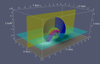Fig. 2. Selected field lines of the TD equilibrium depicting the flux rope (pink) and the surrounding potential field (blue). The two section planes Σ used in Table 1 are the z = 1 plane (cyan) and the x = 0 plane (yellow); see Sect. 5 for details. The distribution of the vertical field component at z = 0 is shown in greyscale at the bottom.

The computation of the vector potentials is performed here using the DeVore gauge A_z = 0; see Sect. 3.2, as implemented in Valori et al. (2012). The method has two parameters, representing different gauges of the DeVore family, as follows. First, a one-dimensional integral in the z-direction is involved in the computation of the vector potentials. This integral can be performed starting from either the bottom (bc = b) or from the top (bc = t) of the considered volume, corresponding to Eq. (10) and Eq. (11) of Valori et al. (2012), respectively. Second, two different boundary conditions can be used in the computation of the vector potential at the starting boundary, namely Eqs. (24) and (25) or Eq. (41) in Valori et al. (2012). As discussed in Sect. 3.2, the latter applied to a potential field results in the DeVore-Coulomb (dVC) gauge. We then use the notation dVC = n (no) and dVC = y (yes) if, respectively, Eqs. (24) and (25) or Eq. (41) in Valori et al. (2012) are used. Therefore, for each vector potential and volume, a different combination of bc and dVC can be used, effectively testing the gauge dependence of the computed quantities. There are four possibilities for each of the six vector potentials, yielding 4⁶ = 4096 possible combinations.

In the following we provide a few representative examples of the possible gauge combinations for each realization of volume splitting. For instance, for test number 2 in Table 1, bc_Ap = [t, t, b] (respectively, bc_A = [t, t, b]) means that the computation of A_p and ${\mathit{A}}_p^a$ (respectively, A and A^a) was performed starting from the top boundary in the volume 𝒱 and 𝒱^a, and from the bottom boundary for ${\mathit{A}}_p^b$ (respectively, A^b) in the volume 𝒱^b. The triplets dVC_Ap = dVC_A = [y, y, y] mean that Eq. (41) of Valori et al. (2012) was used for the computation of all vector potentials in the three volumes 𝒱, 𝒱^a, and 𝒱^b.

5.2. Numerical verification of Eq. (16)

Table 1 summarizes the results of testing Eq. (16) in two representative realizations of volume splitting: in the first one (z = 1, in cyan in Fig. 2) the interface is a horizontal plane cutting through the flux rope at approximately the location of the apex of the flux rope axis. In this realization, most of the flux rope is contained in the lower subvolume 𝒱^a, whereas 𝒱^b mostly contains potential field. The second realization (x = 0, in yellow in Fig. 2) is a vertical plane cutting through the flux rope and approximately containing the flux rope axis. In this realization, the flux rope is split approximately symmetrically between the two subvolumes.

In Table 1, H(B, 𝒱) and

$$\begin{array}{c}\hfill H_{\mathrm{sum}}\equiv H(\mathit{B},{\mathcal{V}}^a)+H(\mathit{B},{\mathcal{V}}^b)+\delta H\end{array}$$(39)

are, respectively, the LHS and RHS of Eq. (16), computed independently, and

$$\begin{array}{c}\hfill ϵ=100\ast (H(\mathit{B},\mathcal{V})-H_{\mathrm{sum}})/H(\mathit{B},\mathcal{V})\end{array}$$(40)

represents the error of the helicity partition formula (Eq. (16)) as a percentage.

In most of the cases in Table 1, the error ϵ in the partition formula is less then 1%, which clearly verifies that Eq. (16) is correct, and that its numerical implementation is extremely accurate. The first three tests in the z = 1 case (test = 1, 2, 3 in Table 1) show that the error ϵ does not depend on the values of the dVC triplets, that is, it is similar for both the deVore and the deVore-Coulomb gauges. This remains true for different combinations of the boundary condition (bc) for the six vector potentials (see tests 4–7 in Table 1). In particular, there is no dependence on the bc value for the vector potential of the potential field. The exception is for bc_A = b in 𝒱^a (see tests 8 and 9), where the error ϵ is around 2%. This gauge corresponds to an upward integration in the computation of the vector potential A^a, that is, to using Eq. (10) of Valori et al. (2012) for A^a. In this case, numerical errors that accumulate in the vertical integration end up affecting the accuracy of the gauge function χ due to Eq. (31). Such analysis is confirmed by the x = 0 cases in Table 1 where some of the tests are repeated for the vertical slice of the volume. Therefore, Table 1 shows that our implementation of Eq. (16) can account for the helicity partition with an error typically smaller than 1%.

In order to attain such accuracy, the computation of the gauge function χ (Eq. (31)), was found to be particularly sensitive. For that, we computed the line integral in a similar way to that shown in Appendix 3 of Valori et al. (2013), that is, such that the integral is the numerical inverse operation of the derivation operator (in our case, a second-order central difference scheme). If, for instance, a trapezoidal scheme is used instead, then ϵ can be easily one order of magnitude larger, or even two in some cases.

In terms of relative magnitude, the values of δH compared to the total helicity H(B, 𝒱), that is with respect to the LHS of Eq. (16), are only about 6% in the z = 1 case, but as large as 74% in the x = 0 case. This is the first evidence that the relative importance of the nonadditive term for a given field depends on how the volume is sliced, and that it can be very significant indeed.

Within a given case, each line in Table 1 corresponds to a different combination of bc and dVC for the six vector potentials, or in other words, to a different gauge. Hence, an estimation of the error for Eq. (16) in fulfilling gauge-invariance can be obtained as the standard error of the mean of δH values. Such a statistical error, relative to the mean of δH, is 5% in the z = 1 case, where δH values are relatively small, and 0.5% for the x = 0 case. Such small variations confirm numerically the gauge-invariance of Eq. (16) within the gauge-invariant accuracy of the underlining helicity computation method (see also the accuracy tests in Valori et al. 2016).

As anticipated in Sect. 3.2, some of the gauge combinations in Table 1 would allow for analytical cancelations in Eqs. (21)–(25). For instance, the second and third tests correspond to the condition ${\mathit{A}}_p^a={\mathit{A}}^a={\mathit{A}}_p^b={\mathit{A}}^b$ on Σ for identical dVC_Ap and dVC_A triplets, which would cancel the first interface term in δℋ_mix of Eq. (25), and set χ = 0 from Eq. (31), yielding δℋ = 0 in Eq. (21) and canceling the last term in Eq. (25). Similarly, each time a “y” is present in the dVC_Ap triplet in Table 1, the DeVore-Coulomb gauge is imposed on one of the vector potentials, and the corresponding term in δℋ_p should vanish. We verified that this is indeed the case to high numerical precision, but the numbers in Table 1 are computed always including all terms in Eqs. (21)–(25). Therefore, they also account for small numerical errors deriving, for example, from a nonperfect solenoidal property of the vector potentials.

5.3. Dependence on the interface position

As a first application of the partition formula, Fig. 3 shows the dependence of the different terms in Eq. (16) as a function of the position of the interface. With reference to Table 1, the gauge used for this application is the same as in test number 3, that is, bc_Ap = bc_A = [t, t, b] and dVC_Ap = dVC_A = [n, n, n].

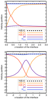Fig. 3. Helicity partition, Eq. (16), for the TD volume split with an interface plane perpendicular to the z-axis (top panel) and to the x-axis (bottom panel) as a function of the interface position. Symbols are the same as in Table 1; see also Sect. 5 for details.

The top panel of Fig. 3 refers to a case where the interface is a plane perpendicular to the z-axis. As the interface height changes from z = 0 to z = 3, its intersection with the TD flux rope rises from the legs, through the apex of the axis of the flux rope at z = 1, until the interface is above the top of the flux rope. To some extent, this numerical experiment is relevant to the study of flux emergence, as it simulates, for decreasing z, the idealized kinematic emergence of a twisted flux tube into the coronal volume, 𝒱^b.

As the height of the interface rises (top panel of Fig. 3), the helicity H(B, 𝒱^a) of the lower volume 𝒱^a (orange curve) and that H(B, 𝒱^b) of the upper volume 𝒱^b (red curve) evolve almost perfectly anti-symmetrically: as 𝒱^a includes more and more of the flux rope, its helicity H(B, 𝒱^a) increases, whereas H(B, 𝒱^b) decreases by a comparable amount. When the interface plane is placed at z = 0.3, the helicity is almost equally distributed between the two subvolumes. The nonadditive term δH (violet curve) is always small for all heights of the interface, with a maximum of 6% of H(B, 𝒱) at z ≃ 1. The accuracy of Eq. (16) is relatively unaffected by the interface position, and H_sum (blue curve) overlaps H(B, 𝒱) (dashed black curve) for all positions of the interface. On the grounds of this first experiment, one would be tempted to say that the nonadditivity term δH tends to be significantly smaller than the helicity of the component subvolumes.

The bottom panel of Fig. 3 shows a similar experiment to that of the top panel but with a vertical plane (perpendicular to the x-axis) that shifts from one side to the other of the flux rope. The change in the helicity of the subvolumes in this case is very different, as it involves a significant variation of δH too. As the interface position moves from x = −3 to x = 0, 𝒱^a increases at the expense of 𝒱^b. In this interval, H(B, 𝒱^b) (red curve) decreases by an amount that is equal to the increase in δH (violet curve), whereas H(B, 𝒱^a) (orange curve), which contains only potential field, is zero, until x ≃ −0.3 where it starts rapidly rising. The TD solution is line-symmetric with respect to the z-axis, and therefore a symmetric evolution is present for x >  0 in the bottom panel of Fig. 3. Indeed, as the interface moves through x = 0 towards x = 1, H(B, 𝒱^a) contains more and more of the flux rope and its helicity H(B, 𝒱^a) increases, mostly at the expense of δH. Symmetrically to the left part of the plot, as soon as the interface moves out of the flux rope, approximately at x = 0.3, H(B, 𝒱^b) is practically zero.

Contrary to the horizontal slicing case in the top panel of Fig. 3, in the vertical slicing case in the bottom panel, δH is of the same order as H(B, 𝒱) for a large interval of the slicing position, and is even several times larger than both H(B, 𝒱^a) and H(B, 𝒱^b) in the central interval: in this case, the nonadditivity term δH is almost never negligible. Therefore, depending on the way a volume is sliced, the relative importance of the nonadditive term δH can vary significantly, and cannot in general be neglected.

From the discussion in Sect. 2.3 we know that the nonadditivity is related to the difference between the reference fields in the subvolumes 𝒱^a and 𝒱^b with respect to the reference field in the full volume 𝒱. On the other hand, the position and orientation of the interface directly determines the boundary conditions for the reference fields. Therefore, the magnitude of δH in the two cases in Fig. 3 is possibly determined by the way in which the boundary conditions for the subvolumes’ reference fields change as a function of the interface position. However, to validate such a speculation requires studying the different nongauge-invariant contributions to δH in Eqs. (21)–(25) as a function of the interface orientation and position, a task that we reserve for future studies; see Sect. 6.3.

6. Conclusions

6.1. Results

The purpose of this work is to study the nonadditivity of the relative magnetic helicity in finite volumes, here formulated as a partition problem between contiguous subvolumes. In particular:

– We derive in Sect. 2.4 the general equation for the partition of relative magnetic helicity in a volume of finite size between two contiguous subvolumes separated by an interface; Eqs. (21)–(25). The explicit assumption of finiteness of the considered volume makes the partition equations directly applicable to numerical simulations. No assumption is made on the shape of the interface or the (sub)volumes, as long as they are simply connected. Therefore, Eqs. (21)–(25) can be easily adapted to different geometries, such as for example spherical wedges and the fully spherical case, taking due care in the required periodicity of vector potentials (i.e. barring any mean field in the periodic direction Berger 2003).

– We show in the most general way that relative magnetic helicity is not an algebraically additive quantity, and that the nonadditive term is gauge-invariant. This allows us to link the nonadditivity to the very definition of helicity as relative to a reference field; see Sect. 6.2.

We then further apply our general equations to specific gauges used in previous studies and numerical computations, as follows.

– In Sect. 3 we analyze the adaptation of the general partition equations to commonly used gauges (Coulomb and DeVore-Coulomb) and boundary conditions often used in the computation of the vector potentials.

– In Sect. 4 we relate our general approach to well-known reference approaches in the literature, such as those by Berger & Field (1984) and Longcope & Malanushenko (2008), which are obtained under more restrictive assumptions on volumes and gauges. In particular, our approach generalizes that of Longcope & Malanushenko (2008) in a few aspects, since all assumptions about the adopted gauge and boundary conditions are relaxed here. In the first place, we use the definition of relative helicity (Eq. (2)) rather than a simple difference of helicities (Eq. (28)). Second, the assumption that subvolumes are bounded by coronal flux surfaces made in Longcope & Malanushenko (2008) implies that the volume must be partitioned in a way that the flux is balanced within the photospheric footprint of each subvolume separately. While this might be a natural way of splitting a coronal volume into a collection of photospherically anchored flux tubes, this might be not an easy task in other types of simulation where the logical split of volumes would not necessarily be following flux surfaces.

– Finally, we implement and test the accuracy and gauge-invariance of the partition equation using the family of DeVore gauges in Sect. 5, applied to the Titov & Démoulin (1999) solution of the nonlinear force-free equations. These preliminary tests, in addition to their verification purposes, show that the nonadditive term is in general non-negligible, and that it can be significantly larger than the relative helicity of the component subvolumes in some cases. However, these tests also show that the magnitude of the nonadditive term depends on the way the volume is split. Therefore, applications of our general formalisms can be devised to investigate under which specific conditions the relative magnetic helicity may become approximately additive (see Sect. 6.3).

6.2. Discussion

The fundamental reason for the nonadditivity of relative magnetic helicity lies in its very definition as relative to a reference field. The very same condition that is needed to ensure the gauge-invariance of relative magnetic helicity (Eq. (3)) is also responsible for the interface discontinuities in the reference fields that ultimately cause the nonadditivity. This is even more evident when the effect of the finiteness of the considered volume must be considered, as in numerical simulations (see, e.g., Valori et al. 2012). We stress that the nonadditive term δH cannot be interpreted as simply the mutual or linking term between the subvolumes, for the same reason that the ℋ_mix term in the definition of the relative magnetic helicity (Eq. (2)) is not the linking term between the input and reference field.

On the other hand, as mentioned in Sect. 1, there are several examples of astrophysical plasmas where the conservation of magnetic helicity is expected to be key to understanding the complex processes at a fundamental level, such as the relation between solar and stellar dynamos and the emergence of magnetic flux through the photosphere, the stability of coronal structure, or the relation between solar eruptions and interplanetary CMEs. In most of these cases, either because of instrumental or numerical limitations, the helicity budget involves volumes that are neither unbounded nor bounded by flux surfaces, and a general, finite-volume approach is unavoidable. The nonadditivity of relative magnetic helicity in finite volumes that we analyze in this work poses a serious threat to the applicability of the conservation of relative magnetic helicity in such fundamental processes. At the very least, our work shows that, when considering the partition of relative magnetic helicity in such applications, the relative magnitude of its nonadditive part must be considered.

Therefore, on a general level, it would be desirable to have a different definition of relative magnetic helicity that has additivity and gauge-invariance as core requirements, which, according to the results in this work, is not possible in general. This impediment does not depend on the type of reference field: as shown in Sect. 2.3, any reference field would lead to the same nonadditivity problem because of the boundary conditions that need to be imposed on the interface in order to ensure gauge-invariance.

It is worth noting that the additivity problem can be solved if one is prepared to relax the requirement of gauge invariance and explicitly fix a gauge in the definition of helicity, as this dispenses with the need for a reference field. The original magnetic helicity ℋ(B, 𝒱) is then (trivially) additive between subvolumes, whatever the gauge of A. However, for this additivity to be useful, one ought to be able to compute the helicity of each subregion locally, whereas in general A must be computed globally (as, e.g., with the Coulomb gauge). Indeed, this problem can be avoided if the interfaces between subdomains are planes or spherical surfaces, because then one can determine a vector potential from B purely by integration within these surfaces. This is the approach of both Prior & Yeates (2014) and Berger & Hornig (2018), who describe particular vector potentials for such configurations. In Prior & Yeates (2014), the interfaces are parallel planes, whereas Berger & Hornig (2018) allow for any spherical nested surfaces. In both cases, the corresponding ℋ(B, 𝒱) is additive between subvolumes and locally computable. Moreover, these authors show that their gauge choices give a particular physical interpretation to ℋ(B, 𝒱), which is lacking for an arbitrary choice of gauge.

6.3. Future applications

Case studies may reveal that the nonadditive term is, in fact, almost negligible in specific conditions. An example of such a case is the kinematic emergence of a flux rope shown in Sect. 5 and top panel of Fig. 3. On the other hand, the bottom panel of the same figure shows that this is not true in general. The reason for such a difference in the magnitude of the nonadditive term is worthy of further investigation. In other words, there might be specific arrangements of fields and interfaces for which δH is indeed nonzero, but still small enough to result in a relative helicity that is approximately additive.

A straightforward application of Eqs. (21)–(25) is to characterise the time evolution of the partition of helicity between sub- and super-photospheric volumes in flux emergence simulations such as, for example Leake et al. (2013). Such a study can be extended to include dynamo simulations (see, e.g., Brun & Browning 2017) and the relation to photospheric fluxes (see e.g., Brandenburg et al. 2017). Similarly, the partition between the helicity carried by an ejective instability and that remaining confined at lower altitudes during solar eruptions can be studied using simulations such as Leake et al. (2014), Pariat et al. (2015b), Török et al. (2018).

On a more theoretical level, our formalism can be used to study the relation between fluxes at the interface of the partitioned volumes and their relation with helicity conservation (see, e.g., Pariat et al. 2015a). Similarly, the relative magnetic helicity proxy recently introduced by Pariat et al. (2017) was found to be a good marker of eruptivity potential in both numerical simulations (Zuccarello et al. 2018) and observed active regions (Moraitis et al. 2019; Thalmann et al. 2019). The eruptivity proxy is expressed in terms of the helicity of the current-carrying part of the field. Intriguingly, the same field appears when combining Eq. (21) and the last term of Eq. (25).

These are only a few examples of applications of our general approach to the partition of relative magnetic helicity. Such applications will help us to understand how the conservation of relative magnetic helicity can be used in practice in the interpretation of the evolution of complex physical processes in magneto-hydrodynamics.

Acknowledgments

G. V. acknowledges the support of the Leverhulme Trust Research Project Grant 2014-051, the support from the European Union’s Horizon 2020 research and innovation programme under grant agreement No 824135, and of the STFC grant number ST/T000317/. L. L., E. P., K. M. acknowledge support of the French Agence Nationale pour la Recherche through the HELISOL project ANR-15- CE31-0001. LL, EP and PD acknowledge the support of the french Programme National Soleil-Terre. A. R. Y. acknowledges financial support from Leverhulme Trust project grant 2017-169 and STFC grant ST/S000321/1. This article profited from discussions during the meetings of the ISSI International Team Magnetic Helicity in Astrophysical Plasmas.

References

Appendix A: Derivation of the nonadditive terms

To allow for cancelations between terms, we split contributions from ∂𝒱^a (respectively, ∂𝒱^b) into contributions from the interface Σ^a (respectively, Σ^b) and contributions from the remaining noninterface boundaries Ʒ^a (respectively, Ʒ^b); see Sect. 2.2.

A.1. Derivation of the δℋ term

Let us start from Eq. (18):

$$\begin{array}{c}\hfill \delta \mathcal{H}={\displaystyle {\int }_{\mathcal{V}}}\mathit{A}·\mathit{B}\mathrm{d}\mathcal{V}-{\displaystyle {\int }_{{\mathcal{V}}^a}}{\mathit{A}}^a·\mathit{B}\mathrm{d}\mathcal{V}-{\displaystyle {\int }_{{\mathcal{V}}^b}}{\mathit{A}}^b·\mathit{B}\mathrm{d}\mathcal{V}.\end{array}$$(A.1)

The solenoidal condition imposes that the normal component of B is continuous across Σ (Berger & Field 1984). However, here we make the more considerable assumption, reasonable in applications, that the vector potential A is continuous with its derivatives at the interface such that the magnetic field B is continuous there (i.e. A|_Σ ∈ C¹ and, hence, B|_Σ ∈ C⁰, at least).

First, we note that

$$\begin{array}{c}\hfill \{\begin{array}{cc}\mathit{B}=\mathbf{\nabla }\times \mathit{A}=\mathbf{\nabla }\times {\mathit{A}}^a\hfill & \forall \mathit{x}\in {\mathcal{V}}^a\hfill \\ \mathit{B}=\mathbf{\nabla }\times \mathit{A}=\mathbf{\nabla }\times {\mathit{A}}^b\hfill & \forall \mathit{x}\in {\mathcal{V}}^b.\hfill \end{array}\end{array}$$(A.2)

Since, e.g., both A and A^a produce the same field in 𝒱^a, then from Eq. (A.2) it follows that they can differ from A at most by the gradient of a scalar function, i.e.

$$\begin{array}{c}\hfill \{\begin{array}{cc}\mathit{A}={\mathit{A}}^a+\mathbf{\nabla }{\chi }^a\hfill & \forall \mathit{x}\in {\mathcal{V}}^a\hfill \\ \mathit{A}={\mathit{A}}^b+\mathbf{\nabla }{\chi }^b\hfill & \forall \mathit{x}\in {\mathcal{V}}^b.\hfill \end{array}\end{array}$$(A.3)

Using the continuity of A and, hence of the RHSs of the above equations, we can split the first integral in Eq. (A.1) into the sum of the integrals on 𝒱^a and 𝒱^b to obtain

$$\begin{array}{c}\hfill \delta \mathcal{H}={\displaystyle {\int }_{{\mathcal{V}}^a}}\mathbf{\nabla }{\chi }^a·\mathit{B}\mathrm{d}\mathcal{V}+{\displaystyle {\int }_{{\mathcal{V}}^b}}\mathbf{\nabla }{\chi }^b·\mathit{B}\mathrm{d}\mathcal{V},\end{array}$$(A.4)

and, by means of Gauss theorem and the solenoidal condition for B,

$$\begin{array}{c}\hfill \delta \mathcal{H}={\displaystyle {\int }_{\partial {\mathcal{V}}^a}}{\chi }^a(\mathit{B}·\mathrm{d}{\mathit{S}}^a)+{\displaystyle {\int }_{\partial {\mathcal{V}}^b}}{\chi }^b(\mathit{B}·\mathrm{d}{\mathit{S}}^b).\end{array}$$(A.5)

We now split the surface integrals into interface and noninterface contributions obtaining

$$\begin{array}{c}\hfill \delta \mathcal{H}={\displaystyle {\int }_{\partial \mathcal{V}}}{\chi }^{\mathit{ab}}(\mathit{B}·\mathrm{d}\mathit{S})+{\displaystyle {\int }_{{\mathrm{\Sigma }}^a}}({\chi }^a-{\chi }^b)\mathit{B}·\mathrm{d}{\mathit{S}}^a,\end{array}$$(A.6)

where we introduced the notation of Eq. (10) for the gauge functions χ^a and χ^b, and we used Eq. (9) in the first integral on the RHS, and that ${\widehat{\mathit{n}}}^b=-{\widehat{\mathit{n}}}^a$ on Σ^b in the second. We anticipate that the first term on the RHS of Eq. (A.6) cancels with the homologous term from δℋ_mix by virtue of Eq. (3), and is therefore omitted from Eq. (21). Then, Eq. (A.6) implies Eq. (21) with χ = χ^a − χ^b.

A.2. Derivation of the δℋ_p term

The explicit form of Eq. (19) is

$$\begin{array}{c}\hfill \delta {\mathcal{H}}_p={\displaystyle {\int }_{\mathcal{V}}}{\mathit{A}}_p·{\mathit{B}}_p\mathrm{d}\mathcal{V}-{\displaystyle {\int }_{{\mathcal{V}}^a}}{\mathit{A}}_p^a·{\mathit{B}}_p^a\mathrm{d}\mathcal{V}-{\displaystyle {\int }_{{\mathcal{V}}^b}}{\mathit{A}}_p^b·{\mathit{B}}_p^b\mathrm{d}\mathcal{V}.\end{array}$$(A.7)

This cannot be computed as δℋ above because, in general, ${\mathit{B}}_p^a$ and ${\mathit{B}}_p^b$ are different from B_p in the volume 𝒱^a and 𝒱^b, respectively. Below, we rather consider explicitly that the reference fields are all potential in their respective domains and must satisfy the gauge-invariance conditions Eq. (3), that is, they satisfy

$$\begin{array}{c}\hfill \{\begin{array}{c}{\mathit{B}}_p=\mathbf{\nabla }\varphi \hfill \\ \widehat{\mathit{n}}·\mathbf{\nabla }\varphi {{|}_{\partial \mathcal{V}}=\widehat{\mathit{n}}·\mathit{B}|}_{\partial \mathcal{V}},\hfill \end{array}\end{array}$$(A.8)

for the reference field in 𝒱, and

$$\begin{array}{c}\hfill \{\begin{array}{c}{\mathit{B}}_p^a=\mathbf{\nabla }{\varphi }^a\hfill \\ {\widehat{\mathit{n}}}^a·\mathbf{\nabla }{\varphi }^a{{|}_{\partial {\mathcal{V}}^a}={\widehat{\mathit{n}}}^a·\mathit{B}|}_{\partial {\mathcal{V}}^a}\hfill \end{array}\mathrm{and}\{\begin{array}{c}{\mathit{B}}_p^b=\mathbf{\nabla }{\varphi }^b\hfill \\ {\widehat{\mathit{n}}}^b·\mathbf{\nabla }{\varphi }^b{{|}_{\partial {\mathcal{V}}^b}={\widehat{\mathit{n}}}^b·\mathit{B}|}_{\partial {\mathcal{V}}^b},\hfill \end{array}\end{array}$$(A.9)

for the reference fields in 𝒱^a and 𝒱^b, respectively.

Let us now use Eqs. (A.8) and (A.9) and the Gauss theorem in Eq. (19) to readily derive

$$\begin{array}{c}\hfill \delta {\mathcal{H}}_p=\delta {\mathcal{H}}_p^{\mathrm{Coul}}+\delta {\mathcal{H}}_p^{\mathrm{Surf}},\end{array}$$(A.10)

where

$$\begin{array}{cc}& \delta {\mathcal{H}}_p^{\mathrm{Coul}}=+{\displaystyle {\int }_{{\mathcal{V}}^a}}{\varphi }^a(\mathbf{\nabla }·{\mathit{A}}_p^a)\mathrm{d}\mathcal{V}+{\displaystyle {\int }_{{\mathcal{V}}^b}}{\varphi }^b(\mathbf{\nabla }·{\mathit{A}}_p^b)\mathrm{d}\mathcal{V}\hfill \\ \hfill & -{\displaystyle {\int }_{\mathcal{V}}}\varphi (\mathbf{\nabla }·{\mathit{A}}_p)\mathrm{d}\mathcal{V},\hfill \end{array}$$(A.11)

$$\begin{array}{cc}& \delta {\mathcal{H}}_p^{\mathrm{Coul}}=+{\displaystyle {\int }_{{\mathcal{V}}^a}}{\varphi }^a(\mathbf{\nabla }·{\mathit{A}}_p^a)\mathrm{d}\mathcal{V}+{\displaystyle {\int }_{{\mathcal{V}}^b}}{\varphi }^b(\mathbf{\nabla }·{\mathit{A}}_p^b)\mathrm{d}\mathcal{V}\hfill \\ \hfill & -{\displaystyle {\int }_{\mathcal{V}}}\varphi (\mathbf{\nabla }·{\mathit{A}}_p)\mathrm{d}\mathcal{V},\hfill \end{array}$$(A.12)

The surface term $\delta {\mathcal{H}}_p^{\mathrm{Surf}}$ can be further reorganized by spitting it into interface and noninterface contributions to obtain

$$\begin{array}{cc}& \delta {\mathcal{H}}_p^{\mathrm{Surf}}={\displaystyle {\int }_{\partial \mathcal{V}}}(\varphi {\mathit{A}}_p-{\varphi }^{\mathit{ab}}{\mathit{A}}_p^{\mathit{ab}})·\mathrm{d}\mathit{S}\hfill \\ \hfill & -{\displaystyle {\int }_{\mathrm{\Sigma }}}({\varphi }^a{\mathit{A}}_p^a-{\varphi }^b{\mathit{A}}_p^b)·\mathrm{d}{\mathit{S}}^a,\hfill \end{array}$$(A.13)

where, in the last term, we have used that ${\widehat{\mathit{n}}}^a=-{\widehat{\mathit{n}}}^b$ on Σ and the notation of Eq. (10) for the scalar potentials ϕ^a and ϕ^b and the vector potentials of the potential fields ${\mathit{A}}_p^a$ and ${\mathit{A}}_p^b$.

A.3. Derivation of the δℋ_mix term

δℋ_mix, Eq. (20), can be written in terms of solely surface integrals using Eq. (6) as

$$\begin{array}{cc}& \delta {\mathcal{H}}_{\mathrm{mix}}={\displaystyle {\int }_{\partial \mathcal{V}}}(\mathit{A}\times {\mathit{A}}_p)·\mathrm{d}\mathit{S}-{\displaystyle {\int }_{\partial {\mathcal{V}}^a}}({\mathit{A}}^a\times {\mathit{A}}_p^a)·\mathrm{d}{\mathit{S}}^a\hfill \\ \hfill & -{\displaystyle {\int }_{\partial {\mathcal{V}}^b}}({\mathit{A}}^b\times {\mathit{A}}_p^b)·\mathrm{d}{\mathit{S}}^b.\hfill \end{array}$$(A.14)

Using the continuity of A and A_p across Σ and the definitions of Eqs. (7)–(9), we can split the first integral on ∂𝒱 into the sum over ∂𝒱^a and ∂𝒱^b by adding and subtracting the interface contributions as

$$\begin{array}{c}\hfill {\displaystyle {\int }_{\partial \mathcal{V}}}={\displaystyle {\int }_{{\mathrm{\Sigma }}^a}}+{\displaystyle {\int }_{{\mathrm{\Sigma }}^b}}={\displaystyle {\int }_{\partial {\mathcal{V}}^a}}+{\displaystyle {\int }_{\partial {\mathcal{V}}^b}}-{\displaystyle {\int }_{{\mathrm{\Sigma }}^a}}-{\displaystyle {\int }_{{\mathrm{\Sigma }}^b}},\end{array}$$(A.15)

and, using Eq. (A.3) to eliminate the vector potential A, we have

$$\begin{array}{cc}& {\displaystyle {\int }_{\partial \mathcal{V}}}(\mathit{A}\times {\mathit{A}}_p)·\mathrm{d}\mathit{S}={\displaystyle {\int }_{\partial {\mathcal{V}}^a}}({\mathit{A}}^a\times {\mathit{A}}_p)·\mathrm{d}{\mathit{S}}^a\hfill \\ \hfill & +{\displaystyle {\int }_{\partial {\mathcal{V}}^b}}({\mathit{A}}^b\times {\mathit{A}}_p)·\mathrm{d}{\mathit{S}}^b\hfill \\ \hfill & +{\displaystyle {\int }_{\partial {\mathcal{V}}^a}}(\mathbf{\nabla }{\chi }^a\times {\mathit{A}}_p)·\mathrm{d}{\mathit{S}}^a\hfill \\ \hfill & +{\displaystyle {\int }_{\partial {\mathcal{V}}^b}}(\mathbf{\nabla }{\chi }^b\times {\mathit{A}}_p)·\mathrm{d}{\mathit{S}}^b\hfill \\ \hfill & -{\displaystyle {\int }_{{\mathrm{\Sigma }}^a}}(({\mathit{A}}^a\times {\mathit{A}}_p)\hfill \\ \hfill & -({\mathit{A}}^b\times {\mathit{A}}_p))·\mathrm{d}{\mathit{S}}^a\hfill \\ \hfill & -{\displaystyle {\int }_{{\mathrm{\Sigma }}^a}}((\mathbf{\nabla }{\chi }^a-\mathbf{\nabla }{\chi }^b)\times {\mathit{A}}_p)·\mathrm{d}{\mathit{S}}^a.\hfill \end{array}$$(A.16)

The identity

$$\begin{array}{c}\hfill \mathbf{\nabla }\times \left({\mathit{A}}_p{\chi }^a\right)={\chi }^a{\mathit{B}}_p+\mathbf{\nabla }{\chi }^a\times {\mathit{A}}_p,\end{array}$$(A.17)

in ∂𝒱^a, and the analogous expression for A_pχ^b in ∂𝒱^b, where all vector fields satisfy the necessary continuity conditions, can be now used to re-write the second line in the RHS of Eq. (A.16) as

$$\begin{array}{cc}& {\displaystyle {\int }_{\partial {\mathcal{V}}^a}}\mathbf{\nabla }\times \left({\chi }^a{\mathit{A}}_p\right)·\mathrm{d}{\mathit{S}}^a+{\displaystyle {\int }_{\partial {\mathcal{V}}^b}}\mathbf{\nabla }\times \left({\chi }^b{\mathit{A}}_p\right)·\mathrm{d}{\mathit{S}}^b\hfill \\ \hfill & -{\displaystyle {\int }_{\partial {\mathcal{V}}^a}}{\chi }^a({\mathit{B}}_p·\mathrm{d}{\mathit{S}}^a)-{\displaystyle {\int }_{\partial {\mathcal{V}}^b}}{\chi }^b({\mathit{B}}_p·\mathrm{d}{\mathit{S}}^b),\hfill \end{array}$$(A.18)

where the first two terms are identically zero because the curl of any (sufficiently continuous) vector field is solenoidal, and the flux through a closed surface of a solenoidal field vanishes. Substituting back into Eq. (A.14),

$$\begin{array}{cc}& \delta {\mathcal{H}}_{\mathrm{mix}}={\displaystyle {\int }_{\partial {\mathcal{V}}^a}}({\mathit{A}}^a\times {\mathit{A}}_p)·\mathrm{d}{\mathit{S}}^a+{\displaystyle {\int }_{\partial {\mathcal{V}}^b}}({\mathit{A}}^b\times {\mathit{A}}_p)·\mathrm{d}{\mathit{S}}^b\hfill \\ \hfill & -{\displaystyle {\int }_{\partial {\mathcal{V}}^a}}{\chi }^a({\mathit{B}}_p·\mathrm{d}{\mathit{S}}^a)-{\displaystyle {\int }_{\partial {\mathcal{V}}^b}}{\chi }^b({\mathit{B}}_p·\mathrm{d}{\mathit{S}}^b)\hfill \\ \hfill & -{\displaystyle {\int }_{{\mathrm{\Sigma }}^a}}(({\mathit{A}}^a\times {\mathit{A}}_p)-({\mathit{A}}^b\times {\mathit{A}}_p))·\mathrm{d}{\mathit{S}}^a\hfill \\ \hfill & -{\displaystyle {\int }_{{\mathrm{\Sigma }}^a}}((\mathbf{\nabla }{\chi }^a-\mathbf{\nabla }{\chi }^b)\times {\mathit{A}}_p)·\mathrm{d}{\mathit{S}}^a\hfill \\ \hfill & -{\displaystyle {\int }_{\partial {\mathcal{V}}^a}}({\mathit{A}}^a\times {\mathit{A}}_p^a)·\mathrm{d}{\mathit{S}}^a\hfill \\ \hfill & -{\displaystyle {\int }_{\partial {\mathcal{V}}^b}}({\mathit{A}}^b\times {\mathit{A}}_p^b)·\mathrm{d}{\mathit{S}}^b.\hfill \end{array}$$(A.19)

Splitting into interface and noninterface contributions we get

$$\begin{array}{cc}& \delta {\mathcal{H}}_{\mathrm{mix}}={\displaystyle {\int }_{{\mathrm{Ʒ}}^a}}({\mathit{A}}^a\times ({\mathit{A}}_p-{\mathit{A}}_p^a))·\mathrm{d}{\mathit{S}}^a+{\displaystyle {\int }_{{\mathrm{Ʒ}}^b}}({\mathit{A}}^b\times ({\mathit{A}}_p-{\mathit{A}}_p^b))·\mathrm{d}{\mathit{S}}^b\hfill \\ \hfill & -{\displaystyle {\int }_{{\mathrm{\Sigma }}^a}}({\mathit{A}}^a\times {\mathit{A}}_p^a)·\mathrm{d}{\mathit{S}}^a-{\displaystyle {\int }_{{\mathrm{\Sigma }}^b}}({\mathit{A}}^b\times {\mathit{A}}_p^b)·\mathrm{d}{\mathit{S}}^b\hfill \\ \hfill & -{\displaystyle {\int }_{{\mathrm{\Sigma }}^a}}({\chi }^a-{\chi }^b)({\mathit{B}}_p·\mathrm{d}{\mathit{S}}^a)\hfill \\ \hfill & -{\displaystyle {\int }_{{\mathrm{\Sigma }}^a}}((\mathbf{\nabla }{\chi }^a-\mathbf{\nabla }{\chi }^b)\times {\mathit{A}}_p)·\mathrm{d}{\mathit{S}}^a\hfill \\ \hfill & -{\displaystyle {\int }_{\partial \mathcal{V}}}{\chi }^{\mathit{ab}}({\mathit{B}}_p·\mathrm{d}\mathit{S}),\hfill \end{array}$$(A.20)

where the continuity of B_p across Σ was used in the third line of the RHS and the notation of Eq. (10) for the gauge functions χ^a and χ^b in the last one. Using the notation in Eq. (10) also for the vector potentials (A^a, A^b) and (${\mathit{A}}_p^a$, ${\mathit{A}}_p^b$), and the definition of Eq. (9), we can formally write

$$\begin{array}{cc}& \delta {\mathcal{H}}_{\mathrm{mix}}={\displaystyle {\int }_{\partial \mathcal{V}}}({\mathit{A}}^{\mathit{ab}}\times ({\mathit{A}}_p-{\mathit{A}}_p^{\mathit{ab}}))·\mathrm{d}\mathit{S}\hfill \\ \hfill & -{\displaystyle {\int }_{{\mathrm{\Sigma }}^a}}(({\mathit{A}}^a\times {\mathit{A}}_p^a)-({\mathit{A}}^b\times {\mathit{A}}_p^b))·\mathrm{d}{\mathit{S}}^a\hfill \\ \hfill & -{\displaystyle {\int }_{{\mathrm{\Sigma }}^a}}({\chi }^a-{\chi }^b)({\mathit{B}}_p·\mathrm{d}{\mathit{S}}^a)\hfill \\ \hfill & +{\displaystyle {\int }_{{\mathrm{\Sigma }}^a}}(({\mathit{A}}^a-{\mathit{A}}^b)\times {\mathit{A}}_p)·\mathrm{d}{\mathit{S}}^a\hfill \\ \hfill & -{\displaystyle {\int }_{\partial \mathcal{V}}}{\chi }^{\mathit{ab}}({\mathit{B}}_p·\mathrm{d}\mathit{S}).\hfill \end{array}$$(A.21)

In the derivation of Eq. (A.21) from Eq. (A.20) we also used Eq. (A.3), the definition χ = χ^a − χ^b, the relation

$$\begin{array}{c}\hfill \mathbf{\nabla }\chi =\mathbf{\nabla }{\chi }^a-\mathrm{\nabla }{\chi }^b=-({\mathit{A}}^a-{\mathit{A}}^b),\end{array}$$(A.22)

and the continuity of A across Σ. We note that, while χ^a and χ^b are defined in the entire subvolumes 𝒱^a and 𝒱^b, respectively, the gauge function χ and Eq. (A.22) are defined only on the interface Σ and are a function of the interface variables only.

The last term on the RHS of Eq. (A.21) cancels with the homologous term in Eq. (A.6) by virtue of Eq. (3), and it is therefore omitted from Eq. (25).

Appendix B: Gauge-invariance of the additivity formula

In this section, we prove the invariance of Eq. (17) with respect to gauge transformations of the vector potentials . First note that each of Eqs. (21)–(25) are invariant if we interchange a ↔ b, since dS^a = −dS^b on Σ. Hence, it suffices to check gauge invariance under gauge changes of A, A_pA^a, and ${\mathit{A}}_p^a$. We consider these gauge transformations in turn:

1. A → A + ∇ψ. We note that A does not explicitly appear in any of the expressions of Eqs. (21)–(25). However, because we are not changing A^a or A^b, transforming A → A + ∇ψ corresponds to the change χ^a → (χ^a + ψ) and χ^b → (χ^b + ψ), as follows from Eq. (A.3). Since nevertheless these potentials appear only in the combination χ^b − χ^a then δH is invariant with respect to the transformation.

References

- Alexakis, A., Mininni, P. D., & Pouquet, A. 2006, ApJ, 640, 335 [NASA ADS] [CrossRef] [Google Scholar]
- Antiochos, S. K. 2013, ApJ, 772, 72 [NASA ADS] [CrossRef] [Google Scholar]
- Berger, M. A. 1984, Geophys. Astrophys. Fluid Dyn., 30, 79 [NASA ADS] [CrossRef] [Google Scholar]
- Berger, M. A. 1999, Plasma Phys. Controlled Fusion, 41, B167 [Google Scholar]
- Berger, M. A. 2003, in Topological Quantities in Magnetohydrodynamics, eds. K. Zhang, A. Soward, & C. Jones (Boca Raton, FL: CRC Press), 345 [Google Scholar]
- Berger, M. A., & Field, G. B. 1984, J. Fluid Mech., 147, 133 [NASA ADS] [CrossRef] [Google Scholar]
- Berger, M. A., & Hornig, G. 2018, J. Phys. A Math. Gen., 51, 495501 [CrossRef] [Google Scholar]
- Berger, M. A., & Ruzmaikin, A. 2000, J. Geophys. Res., 105, 10481 [NASA ADS] [CrossRef] [Google Scholar]
- Brandenburg, A., & Subramanian, K. 2005, Phys. Rep., 417, 1 [NASA ADS] [CrossRef] [Google Scholar]
- Brandenburg, A., Petrie, G. J. D., & Singh, N. K. 2017, ApJ, 836, 21 [Google Scholar]
- Brun, A. S., & Browning, M. K. 2017, Liv. Rev. Sol. Phys., 14, 4 [Google Scholar]
- Del Sordo, F., Candelaresi, S., & Brandenburg, A. 2010, Phys. Rev. E, 81, 036401 [NASA ADS] [CrossRef] [Google Scholar]
- Démoulin, P., & Pariat, E. 2009, Adv. Space Res., 43, 1013 [NASA ADS] [CrossRef] [Google Scholar]
- Démoulin, P., Mandrini, C. H., van Driel-Gesztelyi, L., et al. 2002, A&A, 382, 650 [NASA ADS] [CrossRef] [EDP Sciences] [Google Scholar]
- Démoulin, P., Janvier, M., & Dasso, S. 2016, Sol. Phys., 291, 531 [NASA ADS] [CrossRef] [Google Scholar]
- DeVore, C. R. 2000, ApJ, 539, 944 [NASA ADS] [CrossRef] [Google Scholar]
- Elsasser, W. M. 1956, Rev. Mod. Phys., 28, 135 [NASA ADS] [CrossRef] [Google Scholar]
- Finn, J. H., & Antonsen, T. M. J. 1985, Comments Plasma Phys. Controlled Fusion, 9, 111 [Google Scholar]
- Frisch, U., Pouquet, A., Leorat, J., & Mazure, A. 1975, J. Fluid Mech., 68, 769 [NASA ADS] [CrossRef] [Google Scholar]
- Green, L. M., López fuentes, M. C., Mandrini, C. H., et al. 2002, Sol. Phys., 208, 43 [NASA ADS] [CrossRef] [Google Scholar]
- Jensen, T. H., & Chu, M. S. 1984, Phys. Fluids, 27, 2881 [CrossRef] [Google Scholar]
- Leake, J. E., Linton, M. G., & Török, T. 2013, ApJ, 778, 99 [NASA ADS] [CrossRef] [Google Scholar]
- Leake, J. E., Linton, M. G., & Antiochos, S. K. 2014, ApJ, 787, 46 [NASA ADS] [CrossRef] [Google Scholar]
- Linan, L., Pariat, É., Moraitis, K., Valori, G., & Leake, J. 2018, ApJ, 865, 52 [NASA ADS] [CrossRef] [Google Scholar]
- Longcope, D. W., & Malanushenko, A. 2008, ApJ, 674, 1130 [NASA ADS] [CrossRef] [Google Scholar]
- Matthaeus, W. H., & Goldstein, M. L. 1982, Stationarity of magnetohydrodynamic fluctuations in the solar wind, NASA STI/Recon Technical Report N, 11007 [Google Scholar]
- Moraitis, K., Pariat, É., Savcheva, A., & Valori, G. 2018, Sol. Phys., 293, 92 [NASA ADS] [CrossRef] [Google Scholar]
- Moraitis, K., Sun, X., Pariat, É., & Linan, L. 2019, A&A, 628, A50 [NASA ADS] [CrossRef] [EDP Sciences] [Google Scholar]
- Müller, W.-C., & Malapaka, S. K. 2013, Geophys. Astrophys. Fluid Dyn., 107, 93 [CrossRef] [Google Scholar]
- Nakwacki, M. S., Dasso, S., Démoulin, P., Mandrini, C. H., & Gulisano, A. M. 2011, A&A, 535, A52 [NASA ADS] [CrossRef] [EDP Sciences] [Google Scholar]
- Nindos, A., Zhang, J., & Zhang, H. 2003, ApJ, 594, 1033 [Google Scholar]
- Pariat, E., Démoulin, P., & Berger, M. A. 2005, A&A, 439, 1191 [NASA ADS] [CrossRef] [EDP Sciences] [Google Scholar]
- Pariat, E., Dalmasse, K., DeVore, C. R., Antiochos, S. K., & Karpen, J. T. 2015a, A&A, 573, A130 [NASA ADS] [CrossRef] [EDP Sciences] [Google Scholar]
- Pariat, E., Valori, G., Démoulin, P., & Dalmasse, K. 2015b, A&A, 580, A128 [NASA ADS] [CrossRef] [EDP Sciences] [Google Scholar]
- Pariat, E., Leake, J. E., Valori, G., et al. 2017, A&A, 601, A125 [NASA ADS] [CrossRef] [EDP Sciences] [Google Scholar]
- Priest, E. R., Longcope, D. W., & Janvier, M. 2016, Sol. Phys., 291, 2017 [Google Scholar]
- Prior, C., & Yeates, A. R. 2014, ApJ, 787, 100 [Google Scholar]
- Schuck, P. W., & Antiochos, S. K. 2019, ApJ, 882, 151 [Google Scholar]
- Temmer, M., Thalmann, J. K., Dissauer, K., et al. 2017, Sol. Phys., 292 [Google Scholar]
- Thalmann, J. K., Inhester, B., & Wiegelmann, T. 2011, Sol. Phys., 272, 243 [Google Scholar]
- Thalmann, J. K., Moraitis, K., Linan, L., et al. 2019, ApJ, 887, 64 [Google Scholar]
- Titov, V. S., & Démoulin, P. 1999, A&A, 351, 707 [NASA ADS] [Google Scholar]
- Török, T., Downs, C., Linker, J. A., et al. 2018, ApJ, 856, 75 [Google Scholar]
- Valori, G., Démoulin, P., & Pariat, E. 2012, Sol. Phys., 278, 347 [Google Scholar]
- Valori, G., Démoulin, P., Pariat, E., & Masson, S. 2013, A&A, 553, A38 [NASA ADS] [CrossRef] [EDP Sciences] [Google Scholar]
- Valori, G., Pariat, E., Anfinogentov, S., et al. 2016, Space Sci. Rev., 201, 147 [Google Scholar]
- Woltjer, L. 1958, Proc. Nat. Acad. Sci., 44, 833 [Google Scholar]
- Yeates, A. R., & Hornig, G. 2016, A&A, 594, A98 [NASA ADS] [CrossRef] [EDP Sciences] [Google Scholar]
- Zuccarello, F. P., Pariat, E., Valori, G., & Linan, L. 2018, ApJ, 863, 41 [Google Scholar]