| Issue |
A&A
Volume 642, October 2020
|
|
|---|---|---|
| Article Number | A224 | |
| Number of page(s) | 17 | |
| Section | Planets and planetary systems | |
| DOI | https://doi.org/10.1051/0004-6361/202038758 | |
| Published online | 23 October 2020 | |
Dust trapping around Lagrangian points in protoplanetary disks
1
Instituto de Física y Astronomía, Universidad de Valparaíso,
Chile
e-mail: This email address is being protected from spambots. You need JavaScript enabled to view it.
2
Chinese Academy of Sciences South America Center for Astronomy, National Astronomical Observatories, CAS,
Beijing
100012, PR China
3
Núcleo Milenio de Formación Planetaria (NPF),
Chile
4
Instituto de Astrofísica, Pontificia Universidad Católica de Chile,
Santiago, Chile
5
Universidad Nacional de Córdoba, Observatorio Astronómico – IATE. Laprida 854,
5000
Córdoba, Argentina
6
Departamento de Ciencias, Facultad de Artes Liberales, Universidad Adolfo Ibáñez,
Av. Padre Hurtado 750,
Viña del Mar, Chile
7
Univ. Grenoble Alpes, CNRS, IPAG,
38000
Grenoble, France
Received:
26
June
2020
Accepted:
16
September
2020
Abstract
Aims. Trojans are defined as objects that share the orbit of a planet at the stable Lagrangian points L4 and L5. In the Solar System, these bodies show a broad size distribution ranging from micrometer (μm) to centimeter (cm) particles (Trojan dust) and up to kilometer (km) rocks (Trojan asteroids). It has also been theorized that earth-like Trojans may be formed in extra-solar systems. The Trojan formation mechanism is still under debate, especially theories involving the effects of dissipative forces from a viscous gaseous environment.
Methods. We perform hydro-simulations to follow the evolution of a protoplanetary disk with an embedded 1–10 Jupiter-mass planet. On top of the gaseous disk, we set a distribution of μm–cm dust particles interacting with the gas. This allows us to follow dust dynamics as solids get trapped around the Lagrangian points of the planet.
Results. We show that large vortices generated at the Lagrangian points are responsible for dust accumulation, where the leading Lagrangian point L4 traps a larger amount of submillimeter (submm) particles than the trailing L5, which traps mostly mm–cm particles. However, the total bulk mass, with typical values of ~Mmoon, is more significant in L5 than in L4, in contrast to what is observed in the current Solar System a few gigayears later. Furthermore, the migration of the planet does not seem to affect the reported asymmetry between L4 and L5.
Conclusions. The main initial mass reservoir for Trojan dust lies in the same co-orbital path of the planet, while dust migrating from the outer region (due to drag) contributes very little to its final mass, imposing strong mass constraints for the in situ formation scenario of Trojan planets.
Key words: planets and satellites: formation / planet–disk interactions / protoplanetary disks
© ESO 2020
1 Introduction
In 1772 Joseph-Louis Lagrange identified five equilibrium points (L1, L2, L3, L4, and L5) derived from the restricted three-body problem (Lagrange 1772), in which a particle of negligible mass orbits under the action of two massive bodies (e.g., a star–planet system). Two of these points, L4 and L5, lie in the orbit of the smaller body (planet), each one at the vertex of an equilateral triangle with the opposing joint base formed by the line of the two massive bodies. L4 is located ≃+π∕3 rad at the leading position of the planet, while L5 is located at the trailing co-orbital region at ≃−π∕3 rad (with respect to the planet).
The geometry of L4 and L5 implies thatthe ratio of their distances to the barycenter is equal to the ratio of the two masses. Consequently, the net gravitational force from the planet–star system is zero at these locations. Hence, L4 and L5 should be linearly stable under small perturbations. Gascheau (1843) determined that for sufficiently small ratios (< 1∕27) of the star–planet mass system, it should accumulate nonmassive objects called Trojans (see Brouwer & Clemence 1961; Szebehely 1967; Sosnitskii 1996 for more details on the stability). The first Jovian Trojan (588 Achilles) was discovered by Max Wolf in 1906 (Wolf 1907). Since then, thousands have been reported1. More recently, the first Neptune Trojan asteroids 2001 QR322 and 2008 LC15 (Sheppard & Trujillo 2010) were discovered.
Several efforts have been made to understand the dynamics of Trojans and their origins. For instance, Morbidelli et al. (2005) suggest that Trojan asteroids could have been formed in distant regions to be later captured into co-orbital motion during the migration of the giant planet in the context of the Nice model, where the evolution of the planets is followed after the gas disk hasdissipated (Tsiganis et al. 2005).
The origin of Trojans could also be connected to an even earlier stage of the Solar System, where there is a gas-rich environment. Several hydrodynamical simulations indeed show that asymmetric overdensities in the gas are produced in co-rotation with the planet, favoring L5 over L4 (e.g., de Val-Borro et al. 2006; Lyra et al. 2009). Therefore, the accumulation of Trojan dust should be larger in L5 compared to L4. However, this is contrary to observations of Jovian Trojans, which show a ratio of the number of asteroids N(L4)∕N(L5) ≈ 1.8 for Trojans with diameters D > 2 km (Yoshida & Nakamura 2005).
One possible explanation for this discrepancy is that we now observe the end result of multiple physical processes (e.g., drag forces, collisions, grain growth) that have modified the Trojan population since formation of the Solar System (e.g., Milani et al. 2017). For instance, Di Sisto et al. (2019) analyzed the observed Trojan population through numerical simulations and concluded that the Trojan escape rate from L5 in the lifetime of the Solar System is ~1.1 times greater than that from L4, and is mainly produced by gravitational interactions with the other planets (from Venus to Neptune). Pirani et al. (2019) studied the consequences of planetary migration on the minor bodies of the Solar System through N-body simulations. They find that inward migration produces a more populated leading swarm (L4) than the trailing one (L5), in agreement with observations, while a nonmigrating planet results in symmetric swarms. However, the study of these latter authors is limited by a simplified treatment of the drag force that mimics the effect of the gas-phase of the protoplanetary disk. A complementary explanation could be the lack of systematic observations, or bias in them.
The bias problem concerns two critical aspects. The first is related to the limited amount of time for the observation, which translates to a limitation in the absolute magnitude H that can be reached. For instance, Lagerkvist et al. (2002) show that observing Trojans to a limit of H = 11 mag indicates that the L5 swarm is 75% of L4, while down to H = 13 mag shows that L5 swarm is 76% of L4. The other aspect concerns the covered area to observe a Lagrangian swarm. Unfitted estimations of the density area lead to inaccurate population estimations. For instance, Jewitt et al. (2000) estimate the L4 Trojan population by analyzing an area between L4 and L3, where the distribution is more spread than between L4 and Jupiter. Follow-up observations indicate that their results were overestimated by 40% (Lagerkvist et al. 2002). Different inclination distributions of Trojans and low albedo (e.g., Yoshida & Nakamura 2005) also contribute to bias these detections, notably in the case of small Jovian objects with D ≲ 1 m (e.g., Jedicke et al. 2002). Large correction factors are therefore required to overcome these observational biases (Karlsson 2010).
An interesting scenario is the possibility of a co-orbital planet located at a Lagrangian point. In that context, Lyra et al. (2009) studied the effect of high-pressure regions around the Lagrangian points L4 and L5 of a giant planet. They show that large bodies (m–km) accumulate in tadpole orbits, suggesting the formation of a Trojan Earth-mass planet in situ. This model requires a considerably massive and dense (self-gravitating) disk. In a closely related context, Cresswell & Nelson (2009) investigated the evolution of Trojan planets embedded in a gaseousdisk, from which they can grow to become gas giant planets. The 2D numerical simulations of these latter authors show than once a Trojan planet is placed to grow, the system is stable for about ~ 109 yr.
Despite the strong assumptions needed to produce high-mass Trojan planets, active searches for these objects in extra-solar systems are currently taking place. For instance, Giuppone et al. (2012) analyzed the possible detection of exoplanets in co-orbital motion, namely the TROY project2, an observational and theoretical effort to understand the evolution of planetary systems from the characterization of (still not detected) exo-Trojan planets (Lillo-Box et al. 2018a,b). This characterization raises several open questions, such as: are large Trojan asteroids formed in situ (by aggregates of micron-cm particles to km rocks) or captured, for example during migration? What could be the maximum mass reservoir of dust that can accumulate in Lagrangian points? What is the dynamical evolution of the early dust grains initially present when a protoplanetary object appears?
In this work, we study the early evolution of Trojan dust with the aim being to understand the current configuration of Trojans in the Solar System and the possibility of finding Trojan exoplanets. We model the dynamical evolution of the primordial dust present at the early stage of a gaseous protoplanetary disk, with a particular focus on the dust concentration around the Lagrangian points L4 and L5, and its stability on short timescales (104 yr).
The paper is structured as follows: In Sect. 2, we provide a description of the numerical setup. In Sect. 3, we discuss the physical considerations regarding vortices and Lagrangian points. In Sect. 4, we present the results of the gas and dust simulations. A discussion is provided in Sect. 5, and our main conclusions are drawn in Sect. 6.
2 Numerical model
We follow the evolution of a dusty, gaseous, viscous self-gravitating protoplanetary disk with an embedded planet. For that purpose, we divide our simulations into two stages; the first computes the gas hydrodynamics alone by solving the Navier–Stokes equation and a nonstationary energy equation using a revised version of the 2D FARGO-ADSG code (Masset 2000; Baruteau & Masset 2008). In our version, we model a passively heated disk irradiated by the central star. The disk includes a radiative cooling mechanism assuming black-body radiation, with a nonstationary energy equation. For more details, see Montesinos et al. (2016). The second stage follows the dust dynamics computed on top of the gaseous stage, where the outputs of the hydro-simulation (first stage) are used as inputs for the dust code (second stage), which computes the dynamics of the Lagrangian particles. A complete description of the dust code and our methodology can be found in Cuello et al. (2019).
The evolution of the disk is followed for about 10 000 yr (or 460 planetary orbits). To check that our results correspond to a stationary regime, we also run a supplementary model running up to 1000 orbits for our fiducial model, obtaining almost the same results. We do not present such a model in this work. A description of the dust and gas stage is outlined in the following section.
2.1 First phase: gas dynamic setup
Our fiducial model includes a Jupiter-mass planet located at 7.8 au. The choice of the planet location was motivated by its generated gap, which may be scalable to some observations such as the cavity reported in HD 100546, which could be carved by a Jupiter-mass planet (e.g., Bouwman et al. 2003; Tatulli et al. 2011).
The orbital period of the planet is about Tp = 21.8 yr, and its gravitational effect is introduced smoothly by a taper function such that its final mass is reached after Ntaper = 10 orbits;
![Mathematical equation: \begin{equation*} M_{\textrm{p}}(t)\,{=}\,\begin{cases} M_{\textrm{p}}\cdot \sin^2\left(\frac{\pi}{2}\frac{t}{N_{\rm{taper}}\, T_{\textrm{p}}}\right) & t < 10 \, T_{\textrm{p}} \\[4pt] M_{\textrm{p}} & \textrm{otherwise.} \end{cases} \end{equation*}](/articles/aa/full_html/2020/10/aa38758-20/aa38758-20-eq1.png) (1)
(1)
The initial density profile of the disk is assumed to be
 (2)
(2)
distributed in a radially logarithmic grid of 512 (radial) × 1024 (azimuth) sectors with cylindrical coordinates r, ϕ. The inner radius rin of the disk is located at 2.5 au from the central star, and the outer radius rout at 15 au. From the density profile (2) and the grid limits, the initial disk mass gives  , which is compatible with typical circumstellar disk masses (e.g., Andrews & Williams 2005).
Despite the fact that this mass corresponds to a low disk mass, we include self-gravitating effects in our calculations. These effects could impact the dust dynamics, even for a large Toomre parameter such as that obtained from our disk parameters (Baruteau & Zhu 2016).
We solve a nonstationary energy equation, in which the source term is given by stellar irradiation
 (3)
(3)
where β is the albedo (set to zero), L⋆ the stellar luminosity, and H the scale-height computed assuming local hydrostatic equilibrium  , with cs and vϕ being the sound speed and azimuthal velocity, respectively.
The radiative cooling mechanism is given by black-body emission,
 (4)
(4)
where σSB is the Stefan-Boltzmann constant,  the optical depth, and T the midplane temperature. We simplify our calculations by using a constant disk opacity κ = 1 cm2 g−1. This choice is justified by noting that the Rosseland mean opacity in the temperature and density range of this work gives a mean value κ ~ 1 cm2 g−1 (Semenov et al. 2003).
The disk temperature is initialized by
 (5)
(5)
where h = h0rf is the aspect ratio of the disk. The factor f is the flare of the disk, which is assumed to be f = 1∕7, obtained from equating  , corresponding to a quasi-steady regime. This choice helps to reach a quasi-steady situation as fast as possible. The initial aspect ratio is set to h0 = 0.05. A complete description of the energy equation and its initialization can be found in Montesinos et al. (2016) and Cuello et al. (2019).
To explore other disk configurations we compute different models taking the same density distribution (Eq. (2)), but changing the mass of the planet Mp = {1, 5}MJ, the stellar luminosity L⋆ = {1, 5} L⊙, and the disk turbulent viscosity α = {10−4, 10−3, 10−2}3, where α is the turbulent viscosity prescription from Shakura & Sunyaev (1973). We also run an extra migrating model, where the planet was initially located at 5.2 au. We summarize the explored parameter space in Table 1.
2.2 Second phase: dust dynamics setup
The dust phase is a post-processing calculation where an ensemble of N-independent dust particles react to drag forces produced by the gas and gravitational forces from the star, the gaseous disk, and the embedded planet. The particles are described as Lagrangian test particles that do not interact with one another. The dust code is based on previous work by Paardekooper (2007); Zsom et al. (2011).
The drag force on each particle is computed as
 (6)
(6)
where Ω(r) is the angular velocity of the gas, Δv the relative velocity between the gas and the dust, and St the Stokes number, which is computed as an interpolation between Epstein and Stokes regimes, which is valid for small and large particles, respectively (see Appendix C from Cuello et al. 2019, and Stammler 2017).
Although we use a more convenient way to compute the Stokes number, most of the particles in the simulation follow the Epstein regime, which is valid for particles with sizes smaller than 9/4 of their mean free path (Weidenschilling 1977). In the Epstein regime, the Stokes number for each particle i is given by
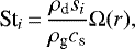 (7)
(7)
where ρd is the bulk density of the dust, si the size of the particle i, ρg the local gas density, and cs the local sound speed. The Stokes number for each particle varies depending on the position r of that particle.
In our calculations, we also include turbulent diffusion of the dust, which is introduced as a random walk of the dust particles. At each time-step d t, particles are displaced in a random direction by a length  , where Dd = αcsH∕(1 + St2) corresponds to the diffusivity coefficient for dust (Youdin & Lithwick 2007).
Our dust simulation uses 150 000 particles. The dust sizes s range from smin = 1 μm to smax = 1 cm, covering the whole dust-size spectrum logarithmically. We set an initial power-law size distribution n(s) ∝ s−1, which gives a power-law dust-density distribution equal to the gas surface distribution. This choice implies approximately the same number of particles perbin size, which allows us to better follow the dust kinematics by directly comparing the assumed dust species. The dust content is introduced at the beginning of the simulation, and is assumed to be a mixture of pyroxene and ices, with an intrinsic bulk density of ρd = 2.0 g cm−3. The initial gas-to-dust ratio is fixed to 100:1.
To calculate a physical quantity such as the effective mass accumulated in a region, or for instance the dust continuum emission, we are required to specify the size distribution n(s) which can be treated as a free parameter, as well as the total dust mass. This free choice does not affect the initial dust size scaling n(s) ∝ s−1, which was chosen for computational reasons. In other words, the simulations give us the spatial distribution of particles, but we need to use a realistic size distribution to compute realistic physical quantities.
Consequently, once the simulation is complete, we re-scale the size distribution by n(s) ∝ s−p, using p = 3.5 (Dohnanyi 1969). Therefore, the dust mass per bin size Mi can be computed as
 (8)
(8)
where ɛ is the initial dust-to-gas mass ratio (i.e., 1:100), and Mgas the total mass gas. The surface density σi for each i-bin can then be computed as
 (9)
(9)
where Ni(r, ϕ) is the number of dust particles per bin size, A(r, ϕ) the surface area of each cell grid, Mi the dust mass per bin size computed above.
Model parameters of the hydro-simulations.
3 Physical considerations
3.1 Vortices
The vortensity gives a measure of the local rotation of the fluid, and its minimum indicates the presence of a local pressure bump. Particles are attracted to higher pressure regions, even for a slight enhancement from the background (Klahr & Lin 2001). Therefore, dust accumulation is expected at the center of vortices (e.g., Barge & Sommeria 1995; Chavanis 2000; Pinilla et al. 2012; Baruteau et al. 2019).
Vortices are expected to appear in the disk as a consequence of Rossby wave instabilities RWI (Lovelace et al. 1999; Li et al. 2000)or baroclinic instabilities Klahr & Bodenheimer (2003). Inside them, pressure maxima are present, with a minimum of the gas vortensity. Typical regions where these instabilities appear, excited by density gradient, are at the edges of the gap carved by a planet (e.g., Lin 2012).
To visualize the vortices generated in the disk, it is useful to compute the amplitude of the vortensity perturbations relative to its initial profile, that is, (ω − ω0)∕ω0. The vortensity field is defined as
 (10)
(10)
where v is the local gas velocity, and ρ = Σ∕H is the vertically averaged density.
As our simulations are in 2D, we simply use ω to refer to the z-component of ω. The quantity ω0 corresponds to the value of the (z-component) vortensity for the initial disk profile.
3.2 Lagrangian points L4 and L5
We are interested in the dust accumulation in the vicinity of the Lagrangian points L4 and L5. To compute their accretion, we need to establish the criterion of dust trapping in the vicinity of those points. A simple approximation can be obtained by solving the three-body problem consisting of two massive bodies of mass M⋆ (primary) and Mp (secondary),where the secondary is moving in circular orbit around their mutual center of mass, and a third particle (test particle of negligible mass) moves in the same plane. Since we are interested in the motion of the test particle, it is convenient to refer to the coordinate system of the particle. In that case, the system is rotating with an angular speed  , where M = (M⋆ + Mp), and a the separation between the two bodies. The dynamic behavior of the third body can be obtained therefore from the effective potential
 (11)
(11)
where r1 and r2 are the distances between the test particle and M⋆, and Mp respectively, and r is the distance to the center of mass of the two bodies (in practice the distance to M⋆). Equation (11) is called the co-rotating effective potential.
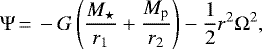
In Fig. 1, we plot the co-rotating equipotential contours from Eq. (11) using the parameter of our simulation: M⋆ = M⊙ and Mp = 5 MJ, both separated by 7.8 au. The figure shows the Lagrangian points L4 and L5 at the planet orbital radius, corresponding to stable equilibrium positions with a zero gradient potential. L4 and L5 are located ~π∕3 radians in azimuth ahead of the planet and behind it, respectively.
Following the contour plot in Fig. 1, we consider that a particle will be in tadpole orbit around a Lagrangian point if it belongs to the cylindrical areas drawn in Fig. 1 that surround L4 and L5. Each cylindrical area is delimited by the position of the Lagrangian points at ± π∕3 adding (or subtracting) an angle of ± π∕8 rad in the azimuthal direction, and between an effective capture radius given by the range rp ± RHill, that is,
![Mathematical equation: \begin{align}& \pi/3 ~ (L_4) - \pi/8 < \phi < \pi/3 ~ (L_4) + \pi/8,\\[2pt] & -\pi/3 ~ (L_5) - \pi/8 < \phi < -\pi/3 ~ (L_5) + \pi/8,\\[2pt] & r_{\textrm{p}} - R_{\textrm{Hill}} < r < r_{\textrm{p}} + R_{\textrm{Hill}},\end{align}](/articles/aa/full_html/2020/10/aa38758-20/aa38758-20-eq18.png)
where rp is the planet radial location and RHill is the Hill radius4. We show a posteriori that the libration of particles around a Lagrangian point occurs in such a pre-defined area.
At each time-step, we count particles that enter and leave the defined region. This method enables us to calculate the net dust flux in L4 and L5. At late evolutionary stages of the disk, when a stationary regime is reached, the Lagrangian points neither accumulate nor lose material.
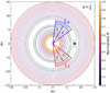 |
Fig. 1 Equipotential lines according to Eq. (11) in a rotating frame with the planet, applied to a model with parameters M⋆ = 1 M⊙, rp = 7.8 au, and Mp = 5 MJ. The leading Lagrangian point (L4) is located at + π∕3, while the trailing point (L5) is at − π∕3. A stable librating azimuthal angle is assumed to be ±π∕8 around eachLagrangian point. |
4 Results
4.1 Gas and dust evolution
Figure 2 shows the evolution of the disk model 1 for the timescales 46, 230, and 459 orbits (as one planetary orbit takes 21.8 yr, this corresponds to 1000, 5000, and 10 000 yr, respectively), the different subplots include: the gas density, dust density, particle distribution, and gas-to-dust ratio for all the sizes ranging from 10−4 to 100 cm. All models start with a gas-to-dust ratio equal to 100:1.
During the evolution, we observe the formation of an inner disk and an outer one as the planetary gap develops, along with typical density wakes at the Lindblad resonances. By the end of the simulation, the planet practically depletes the co-rotating zone from gas (bottom of Fig. 2). As expected, the dust evolves differently depending on its coupling to the gas.
At 46 orbits (upper-panel, Fig. 2), a gap is already present in the disk. However, a horseshoe structure of dust with particles of all sizes populates the co-rotating zone. The dust density inside the gap is very low ~ 0.003 gr cm−2, with a gas-to-dust ratio of ~528 : 1, except at the two Lagrangian points, where the gas-to-dust ratio is reduced to 13:1 (L4) and 9:1 (L5), indicating dust accumulation. In the outer disk, two blobs of dust appear, corresponding to two vortices (see Sect. 4.2). The vortices are not noticeable in the gas. The gas-to-dust ratio at the large swarm reach ~ 8 : 1 (Fig. 2: coordinates x ~−7;y ~−8 au), showing efficient dust trapping.
After 230 orbits (middle panel, Fig. 2), the gap is more depleted of gas, while the co-rotation zone is still populated by dust of all sizes. The mm–cm particles inside this region continue to accumulate around the Lagrangian points. The gas-to-dust ratio in these points is reduced to 4.4:1 (L4) and 3.8:1 (L5). The two dusty blobs present in the outer disk at 46 orbits have collided to form a single one (located at coordinates x ~ 10; y ~ −5 au), with a total mass of 16.3 Mmoon, and a gas-to-dust ratio of about 13.8:1.
At the end of the simulation (orbit 459, bottom panel, Fig. 2), μm and submm particles are librating in horseshoe orbits around L4 and L5, while mm–cm particles are confined in tadpole orbits around either L4 or L5. From Fig. 2 (orbit 459), the leading swarm (L4) accumulate more small particles than the trailing Lagrangian point (L5). However, there is more mass accumulated in L5 than in L4 since most of the mass is concentrated in large particles (mm–cm), which are concentrated mostly around L5.
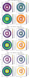 |
Fig. 2 Evolution of the gas and dust in model (1), for three evolutionary stages; 46, 230, and 459 orbits. The dust panels show the full size range of the particles, from 10−4 to 100 cm. The panels have been rotated to always keep the planet at the same location x = 7.8 au, y = 0. |
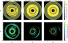 |
Fig. 3 Top: Evolution of the vortensity and dust in model 1, for three evolutionary stages: 46, 230, and 459 orbits. Bottom: Dust distribution of particles with sizes in the range 10−2 − 100 cm. The planet rotates in the counter-clockwise direction. The panels have been rotated to always keep the planet at the same location, namely x = 7.8 au, y = 0. |
4.2 Vortices
Figure 3 shows the amplitude of the vortensity deviations from the background for model 1, that is, (ω − ω0)∕ω0, where Eq. (10) was used to compute ω for the outputs: 46, 230, 460 orbits. For comparison, we plot the dust distribution by sizes next to the vortensity. For a better analysis, we divide the disk into three regions: (a) the inner disk, (b) the gap, and (c) the outer disk, as described below.
- (a)
In early stages, the inner disk shows a homogeneous vortensity, with a local minimum (blue color) developing at the edge of the inner disk just next to the gap. The bottom panel of Fig. 3 shows the size distribution of dust, where sub-millimeter to cm particles (yellow color) are observed. As the disk evolves, two dusty rings concentrating submm to cm grains develop. The location of such rings coincides with the location of the minimum in vortensity.
- (b)
The gap exhibits a local minimum vortensity with a typical horseshoe structure, trapping submm and cm sizeparticles. At early stages, two prominent vortices are identified at the Lagrangian points L4 and L5, where L5 covers a larger area than L4 (two blue islands observed in the gap). Hence, the Lagrangian points start to collect large particles (mm–cm). The vortices persist during the simulation, trapping more dust particles as the disk evolves. Trojan dust of 10−2−100 cm lies in L4 and L5 at the end of the simulation.
- (c)
Initially, the external disk exhibits two notorious vortices (blue islands), which start to trap dust. With time, the two vortices collide to form one single vortex, resulting in a larger banana-shaped vortex, concentrating submm to cm particles. The dust mass of the final outer lobe or satellite reaches ~ 16.6Mmoon with a gas-to-dust ratio of about 9:1. One should note that the dust distribution in Fig. 3 only shows submm to cm grains because these sizes are effectively trapped in the local pressure maximum and vortices.
At the end of the simulation, mm to cm particles have been efficiently trapped at the Lagrangian points by small vortices created by the planet–star system. The vortices continue to be present at the end of the simulation although the size of the now-single vortex has reduced over time. If there were more material within the gap, the slightly higher pressure at the center of the vortices would continue to trap dust. Besides the populated Lagrangian points, two concentric rings at the inner region develop. These are dust traps created by planetary wakes.
4.3 Dust accumulation by sizes around Lagrangian points
4.3.1 Gas–dust interaction
Figure 4 shows the evolution for each dust bin size (μm to cm) at different evolutionary stages: 300, 2 000, 4 000, 6 000, and 10 000 yr. We observe that the largest particles in the range of0.3–1 cm (yellow) quickly accumulate at the Lagrangian points. In less than 1000 yr (45 orbits), L4 and L5 are already settled, including a forming system of two inner rings (at ~4 au), originated from planetary wakes. On the same timescale, small particles in the range of 10−1.5−10−1 cm (green color) are also trapped at the Lagrangian points. At the end of the simulation, a relatively massive swarm of dust of ~ 16.6 Mmoon is formed bymm–cm particles (yellow/green) located at the outer region showing a banana-shaped dust concentration. The swarm corresponds to the leftover of the extinct external dusty disk.
Particle sizes in the range of 10−2.5–10−1.5 cm (green–blue) behave in a slightly different fashion. A horseshoe starts to develop at 1000 yr. As the disk evolves, a gap is carved by the planet. Soon, the gap reduces its number of green–blue particles, which remain mostly trapped at the Lagrangian points. An external disk is also created as the dust evolves. The external swarm of 16.6 Mmoon described above is hidden in this outer ring of 10−2.5–10−1.5 cm particles. Micrometer to 10−2.5 cm (blue–violet) particles are distributed all over the disk; in the inner disk, within the gap (librating in horseshoe orbits around L4 and L5), and in the outer disk.
Once the simulation ends, we analyze the distribution of particle size and Stokes number around the Lagrangian points, computing how much material is finally concentrated in L4 and L5. In Figs. 5 and 6, we plot the mass spectrum of L4 and L5 for model 1, and their ratio L4∕L5 after 10 000 yr (460 orbits) of evolution as a function of particle size and Stokes number, respectively.
In Fig. 7, we plot the accumulated effective mass per radial bin. We notice that centering an annulus at the planet location rp, the capture area extends from rp + 2RHill towards the outer region, and rp − 1.5RHill towards the star. However, the effective capture radius, defining tadpole orbits, is mostly inside rp ± RHill as defined by Eq. (14).
We observe the following interesting features from the mass spectrum: (i) There is an asymmetry in the total mass accumulated in each Lagrangian point. L4 accumulates 2.1 Mmoon, while L5 accumulates 3.0 Mmoon (Figs. 5 and 7). (ii) Most of the effective mass trapped in L4 and L5 is found in particles in the range of ~0.03 to 1 cm (top panel of Fig. 5). A small amount of micron-sized particles are also trapped in the Lagrangian points. (iii) The mass asymmetry between L4 and L5 depends on the particle size. Small particles in the range 10−4 to 10−1.5 cm are more abundant in L4, while particle of 10−1.5 to 1 cm are more abundant in L5 (see bottom panel of Fig. 5). The transition (when mass in L4 is equal to that in L5) happens for 10−2 cm particles. However, the effective mass (all sizes) is always larger in L5 than L4. (iv) The range of the Stokes number of particles trapped in the Lagrangian points lies in the range St ~ 10−6−10. Particles trapped in L4 (small particles) are dominated by Stokes number St < 0.1. Particles with large Stokes numbers, that is with St > 0.1, are commonly trapped in L5.
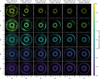 |
Fig. 4 Evolution in time of the dust for model 1 as a function of particle size, ranging from μm to cm. The panels have been rotated to always keep the planet at the same location x = 7.8 au, y = 0. |
4.3.2 Mass accretion at Lagrangian points
The dust accumulation rate around a Lagrangian point differs depending on the specific particle size. Figure 8 shows mass as a function of time in the vicinity of Lagrangian points for a specific range of sizes for model 1, that is: 10−4−100, 10−4−10−3, 10−3−10−2, 10−2−10−1, and 10−1−100 cm. Initially, the total dust mass grows exponentially. During the first 50 planetary orbits, L5 accumulates ~ 2.7 Mmoon of dust, while L4 reaches about ~ 1.9Mmoon, where the main contribution of the mass comes from the largest particle size, namely, 10−1−100 cm. After that, the accretion rate is almost completely halted, reaching its final mass of 2.13 Mmoon for L4, and 3.0 Mmoon for L5.
Lagrangian points are almost completely depleted of micron-size particles. Figure 8 shows that particles in the range of 10−4−10−3 cm do not contribute to the mass trapped in L4 and L5. The generated vortex at the Lagrangian points is not strong enough to attach stable orbits for this size range. However, a considerable amount of gas is located around L4 and L5, namely 4.8 Mmoon of gas in L4, and 5.6 Mmoon in L5 (with mean gas density of ~0.4 and ~0.5 g cm−2 respectively), which is responsible for the pressure bump trapping mm–cm dust. At the end of the simulation, the gas-to-dust ratio is 2.2:1 for L4 and 1.9:1 for L5.
Table 2 summarizes the dust properties at the Lagrangian points at the end of each simulation, for all the models in Table 1.  represents the accumulated dust mass,
  the dust density, Σgas∕σdust the gas-to-dust ratio, and ⟨T⟩ the mean dust temperature, where we assume that the dust has the same temperature as the gas. All these quantities are evaluated at each Lagrangian point L4 and L5, inside the effective capture region given by Eqs. (12)–(14).
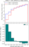 |
Fig. 5 Mass spectrum of model 1 as a function of the size of the dust accumulated in L4 and L5 for thelast evolutionary stage (460 orbits). The bottom panel shows the mass ratio L4 ∕L5 as a function of dust particle size. |
4.4 Instabilities at the Lagrangian points
Our fiducial model (model 1) shows a relatively stable behavior of mass accumulation at the Lagrangian points (Fig. 8). We explore the impact of turbulent viscosity α, planetary mass Mp, and stellar irradiation L⋆ on the stability of trapped dust. We present our findings below.
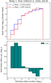 |
Fig. 6 Mass spectrum of model 1 as a function of the Stokes number for the dust accumulated in L4 and L5 at the last evolutionary stage (460 orbits). The bottom panel shows the mass ratio L4∕L5. |
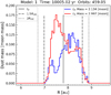 |
Fig. 7 Histogram of the effective dust mass accumulated at the end of the simulation inside L4 and L5, distributed by radial bins. This defines a capture region given by rp + 2RHill from the planet towards the outer region, and rp − 1.5RHill from the planet towards the star. An effective capture radius is expected at rp ± Rhill. |
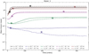 |
Fig. 8 Dust mass accumulated in time around the Lagrangian points L4 (continuous line) and L5 (dotted line) for model 1. The evolution is shown for different sizes, including the effective (all sizes) accumulated mass (black continuous line). |
Dust properties at the Lagrangian points L4 and L5 computed forthe last evolutionary stage (460 orbits).
4.4.1 Effect of turbulent viscosity
The situation is somewhat different if the turbulent viscosity is increased. Models 1, 2, and 6 share the same parameters, apart from the viscosity: α = 10−4 (model 1), α = 10−2 (model 2), and α = 10−3 (model 6) (see Table 1).
In Fig. A.1, we plot the dust-mass evolution around L4 (solid line) and L5 (dotted line) for model 2. In this enhanced viscosity model (α = 10−2), the effective mass reaches final values of 0.6 (L4) and 2.2 (L5) Mmoon. This is in stark contrast to the accumulated mass in the low viscous model 1 (α = 10−4), where the final mass reaches 2.1 (L4) and 3.0 (L5) Mmoon.
Another remarkable difference from model 1 is that the only particles that effectively accumulate in both Lagrangian points are in the range of 0.3–1 cm. Small particles in the range of 10−2−10−1 cm accumulate in L4 and L5 for a short period only. An instability is triggered after 200 orbits, evacuating these particles from the Lagrangian points (Fig. A.1). When the gap is being carved, small particles initially located in co-rotating orbits are dragged towards the inner disk by gas accretion. They never follow stable tadpole orbits around the Lagrangian points for such a high-viscosity model. Furthermore, increasing the gas viscosity increases the transport of angular momentum, promoting gas accretion towards the star. The enhanced accretion produces a less active vortensity. The less active vortex does not retain the smaller (10−4−10−2 cm) particles efficiently.
There is also the effect of diffusion of dust particles. In our simulations, such diffusion is modeled through the coefficient Dd = αcsH∕(1 + St2), which is proportional to the turbulent α-viscosity. The enhanced viscosity promotes radial diffusion of particles, helping to trigger the observed instabilities, and making the accumulation of dust particles more difficult in the Lagrangian points. However, despite having the effect of higher turbulent viscosity and a diffusive mechanism for particles, we still have a significant accumulation of mm–cm particles in L5.
Figure A.5 (top panel) shows the mass spectrum of the dust accumulated in the Lagrangian points for model 2. The bottom panel shows the mass ratio L4∕L5 per bin size. The total mass ratio gives 0.3 (compared to 0.7 for model 1). This comparison suggests that a higher turbulence in the disk stimulates the evacuation of dust grains from L4 rather than L5 (therefore the mass ratio L4∕L5 is reduced for high-viscosity models). In other words, the lower the viscosity, the greater the similarity between L4 and L5 in terms of dust mass.
With an intermediate value for the turbulent viscosity (α = 10−3, model 6), we find an intermediate situation between model 1 (α = 10−4) and model 2(α = 10−2). See Fig. A.2 for the dust accumulation rate, and Fig. A.6 for the final mass spectrum of model 6.
4.4.2 Effect of planetary mass
In model 3, the mass of the planet is increased to 5 MJ, keeping the same parameter space as in model 1. The massive planet of model 3 carves a broader gap by a factor  (Kanagawa et al. 2016), and on a shorter timescale compared to model 1. Gravitational perturbations from the planet severely affect the evolution of dust particles around the Lagrangian points.
Figure A.3 shows the dust evolution around L4 (solid lines) and L5 (dotted lines) for model 3. In this case, only L5 accumulates grains, where most of them are large particles in the range 10−1−100 cm.
The rapid formation of the gap for this model leads to an enhanced evacuation of gas inside the co-rotation zone, through a region slightly closer to the leading zone of the planet, thereby removing most of the particles attached to L4. The larger the planetary mass, the less efficient the dust capture at a Lagrangian point.
4.4.3 Effect of stellar irradiation
Comparing models 3 and 4 reveals some aspects of the influence of stellar irradiation. Model 3 has a central star with 5 L⊙, while model 4 is a colder model with 1 L⊙. In Model 3 (described in Sect. 4.4.2, particles at L4 are completely decoupled after 200 orbits of evolution. For a colder model such as model 4, particles that once accumulated around L4 also become unbound as a consequence of the huge gap created by the massive 5 MJ planet), but at a later evolutionary stage, after 340 orbits (compared to 200 orbits for the hotter model 3). The broader gap leads to particles decoupling from L4 anyway. In a colder disk, the pressure scale-height is smaller, making it easier for a planet to open a gap and produce variations in the pressure field with sharper transitions in the radial direction, which translates to the promotion of RWI and hence the formation of vortices that last longer.
4.5 Evolution and trajectory of dust particles
For better visualization, we divide the last evolutionary stage of model 1 into three regions: (a) inner ring, (b) the gap, and (c) the outer disk. Each zone features different morphologies worth studying (see Fig. 4). We randomly select a number of particles of different sizes from the last step of the simulation belonging to specific zones of the above three regions and trace back along their evolutionary path, starting from the initial time-step to the last one.
4.5.1 Inner ring
At the inner rim of the disk, two concentric mm–cm dusty rings produced by planetary wakes are located at r ~ 3.8, and r ~ 5.6 au, revolving at resonances of 3:1 (3.8 au) and 5:3 (5.6 au), respectively, with respect to the planet. The rings are clearly visible at the end of the simulation (top right panel of Fig. 4).
We selected particles belonging to the second dusty ring at r = 5.6 au (for the output 459 orbits, model 1) and traced back their trajectories. Figure 9 shows the evolution of their radial position as a function of time, starting at t = 0 to t = 10 000 yr. The color bar indicates the size of each particle. The two horizontal red lines indicate the position of the Lagrangian libration zone (the planet is located at rp = 7.8 au). The particles that end up trapped at the inner ring (r = 5.6 au) came from different regions of the disk, initially located between the radii at 5.5 au and 8.8 au (see t = 0 in Fig. 9).
The mm–cm particles beyond 6.5 au migrate due to drag forces to their final position at 5.6 au (Fig. 9), while μm particles of this ring were initially located at the same original radial distance (close to 5.6 au), oscillating with an amplitude of ~ 1 au around r ~ 5.6 au while they travel through the full orbital path around the star. A few μm particles were initially found at the co-rotation zone of the planet; being coupled to the gas, these particles were relocated to the inner ring by gas accretion. It is interesting to note that the ring located at r ~ 5.6 au is rather composed of two close small rings; one accumulates submm particles, while the other accumulates mm–cm particles.
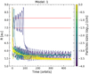 |
Fig. 9 Radial trajectory of randomly selected particles (μm to cm) that end up trapped in the second inner ring located at r = 5.6 au featured at the end of the simulation in model 1. |
4.5.2 The gap: tadpole and horseshoe orbits
We are interested in the libration of particles around L4 and L5, including tadpole and horseshoe trajectories between both locations. We selected several particles from the last output in the size range 10−4−100 cm that end up trapped inside the librationarea of L4 defined by the azimuthal position: π∕3 − π∕8 < ϕ < π∕3 + π∕8, and radius: rp − RHill < r < rp + RHill (see Sect. 3.2, Eq. (12)). Figure 10 shows the evolution in time of the radial and azimuthal coordinates of each particle. The horizontal red lines in Fig. 10 indicate the defined libration area.
As soonas these particles start their motion, they engage into a damped oscillation mode between the capture region rp ± Rhill ~ (Rhill ~ 0.5 au for model 1). The larger the particle size, the larger the damping. Millimetric and centimetric particles become immediately constrained to oscillate very close around rp (under-damped regime). Submm and μm particles also oscillate in an under-dumping mode but with a larger amplitude around rp (see top panel of Fig. 10). Regarding the azimuthal coordinate, mm and cm particles oscillate with small amplitude around a full orbit around the star; they quickly reach the equilibrium position at L4 (recall that we selected only particles ending up in L4; see particlesinside the horizontal red lines at the bottom panel of Fig. 10). However, small particles (μm and submm) librate with larger amplitudes. Some of them become trapped in the other Lagrangian point L5 for a while, going back and forth from L4 to L5, before finally ending up inL4.
In summary, mm–cm particles that end up in L4 oscillate around L4 (tadpole orbits) during the whole simulation with an amplitude defined by the libration amplitude (Eq. (12)). Submm and μm particles oscillate around both Lagrangian points (horseshoe orbits). L4 catches more smaller particles (μm–submm), and L5 efficiently traps larger particles (mm–cm).
A major result is that all particles that end up at L4 (or at L5), regardless of their size, were initially located inside the libration region defined by the effective capture radius (Eq. (14)), that is, an annulus centered at rp with a width of Δr = 2 × RHill (~ 1 au for model 1). No particles initially located outside this area end up trapped around a Lagrangian point. Particles traveling from outer regions dragged by the gas pass through the gap but without being trapped in tadpole orbits around a Lagrangian point. The capture region suggests that the mass reservoir to be accumulated in a Lagrangian point should be 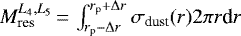 , where σdust(r) is the initial dust density profile, and rp the planet position.
This maximum imposes some constraint on the in situ formation scenario of Trojan planets. For instance, from the initial condition defined for model 1 (Sect. 2.1, Eq. (2)), we have σdust(r) = Σgas(r)∕100, which gives 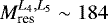 Mmoon (2.3 Earth masses). For this model, the final masses around L4 and L5 are 2.13 and 3.0 Mmoon, respectively (see Table 2), representing a capture efficiency of about 1.2% (L4) and 1.6% (L5) of
  . Depending on the simulation parameters, the capture efficiency may vary. However, the mass reservoir is an independent constraint, which will not change when varying the parameters or if a larger or smaller disk is assumed.
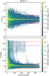 |
Fig. 10 Trajectories of some particles (μm to cm) from model 1 that end up trapped inside the Lagrangian point L4 only. The top horizontal red lines represent the location L5, while the bottom horizontal lines represent L4. Some submm particles oscillate in horseshoe orbits (between both L4 and L5) before ending in L4. Large mm–cm particles oscillate only in tadpole orbits around L4. |
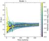 |
Fig. 11 Radial trajectory of randomly selected particles (μm to cm) that end up trapped in the outer ring located at r = 11 au featured at the end of the simulation model 1. |
4.5.3 Outer disk
The outer disk shows a wide ring structure located at r ~ 11 au composed of μm and submmparticles. Within this ring, a large vortex is produced as a consequence of the gravity of the planet, with an over-density of mm–cm particles with a total mass of 16.6 Mmoon (bottom-right panel of Fig. 3).
We selected some of the trapped grains in the vortex to trace their trajectories back in time. Figure 11 shows the evolution of those particles starting from t = 0 to t = 10 000 yr. We find that the particles were initially located at radial positions between 8.8 to 15 au (the vortex is located at r ~ 11 au).
Some large (mm–cm) particles migrate outward, driven by forces from planetary wakes, while others migrate inward, influenced by drag. Submm dust particles trapped in the vortex were initially located only in orbits close to its final position inside the vortex, that is, r~ 11.5 au (see Fig. 11).
As shown in Fig. 11, mm–cm particles barely oscillate in the radial direction while they travel through the disk. In contrast, small, submm particles oscillate with decreasing amplitude in the radial direction while they move toward the vortex.
Analyzing the vortex dynamics as a whole, we find that at t = 1000 yr, it revolves with a mean motion resonance (MMR) of 3:2 with respect to the planet, shifting radially to its final position at r ~ 11 au reaching an MMR of 5:3 at the end of the simulation. The resonant vortex, with its dusty banana-shaped structure (bottom panel of Fig. 3), could feature some observational signatures such an asymmetry in the dust continuum of the dusty ring to which it belongs, peaking in scattered infrared light and submm emission (e.g., Bae et al. 2016; Baruteau et al. 2019). However, further radiative analysis is beyond the scope of this work.
In our simulations, the planet was not able to migrate. However, for completeness, we run two dedicated models: (i) one in which a 10 MJ planet ‘feels’ the disk, starting a type II migration regime; (ii) and an identical model, but without migration (see parameter Table 1, models 7 and 8). It is worth mentioning that, in general a massive planet migrates faster than a lower mass planet. For instance, at first order, a reference migration timescale would be  (e.g., Armitage 2010). In our simulation, a 10 MJ planet starts a fast inward type II migration regime from 5.2 to 3.7 au in 460 orbits.
The effect of planet migration slightly reduces the total mass accumulated in both L4 and L5, but the asymmetry favoring L5 over L4 remains. Migration does not enhance material accumulation in L4 over L5, or trigger any destabilization mechanism around L5 as proposed by Gomes (1998). The only difference we find is on the trajectories of micron particles coupled to the gas. Those particles are not captured in stable tadpole orbits in the horseshoe region, which is probably because of the large planetary mass used (needed to obtain a fast type II migration regime).
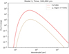 |
Fig. 12 Spectral energy distribution from the disk, and the Lagrangian point L5 from model 1 computed at the last evolutionary stage. Emission from the Lagrangian point comes from an optically thin dusty swarmof ~3 Mmoon with a mean temperature of ~55 K. |
4.6 Radio flux from Lagrangian points
From the last outputs of the simulation, noting that the system has reached a quasi-stationary regime, we can estimate the emission from the disk and the Lagrangian points. Assuming that the source is located D = 150 pc away, the total disk flux can be estimated by integrating the Planck function Bν over the disk surface;  , obtaining a peak flux of about ~450 mJy at 50 μm for model 1. On the other hand, the dust accumulated in a Lagrangian point contributes with a specific localized emission. If it comes from an optically thin region, the emission can be computed from Fν = (1∕D2)MdustκνBν(T), where Mdust corresponds to the dust mass located at the Lagrangian point, and T its temperature (Hildebrand 1983). Using the values from Table 1 (Mdust ~ 3Mmoon, T ~55K), we obtain for model 1 an integrated flux of ~20 mJy also peakingat 50 μm. This is an idealized estimation, without taking noise or instrument limitations into account. The spectral energy distribution for this model is shown in Fig. 12.
5 Discussion
We studied the evolution of dust present in a viscous disk with an initial gas-to-dust ratio of 100:1. The disk has an embedded approximately Jupiter-mass planet located at 7.8 au which we follow for 460 orbits. The dust is treated as Lagrangian particles with a full spectrum of sizes ranging from 10−4 to 100 cm. Our simulations are done over two stages: The first one computes the gas dynamics by solving the Navier–Stokes equations, including a nonstationary energy equation for an irradiated disk. The second stage computes the dust dynamics in which dust particles ‘feel’ the gravity from both the star and the planet, and the drag caused by the gaseous disk.
We mainly focus on dust dynamics around Lagrangian points L4 and L5, examining the impact of three parameters that play an important role in the evolution of the dust: the mass of the planet Mp, the turbulent viscosity of the gas α, and the stellar irradiation (to heat the gas) from the star L⋆. Some general conclusions, independent of the parameter choice, arise from these models: Once the planet has carved a gap in the disk, two vortices appear located at the Lagrangian points L4 and L5, revealed by the vortensity minima (Fig. 3). These minima act as dust traps (Crnkovic-Rubsamen et al. 2015; Surville et al. 2016), accumulating material in the librating region around L4 and L5. In all the models, we find that L4 invariably captures a larger number of small (μm-submm) dust grains than to L5. On the other hand, mm and cm particles are always more abundant in the trailing L5 Lagrangian point. Larger particles account for more mass; therefore, we always find that at the end of the simulation, L5 has accumulated more mass than L4. Typical values of the mass accumulated around L5 are on the order of 2–3 Mmoon.
The observed asymmetry applies to all the models, consistent with past theoretical works suggesting that in the presence of drag, the orbits of Trojans around L5 are more stable than those around L4 (e.g. Peale 1993; Murray 1994). The origin of this asymmetry is due to an over-density created at the trailing region of the planet (e.g., de Val-Borro et al. 2006; Lyra et al. 2009). Such an over-density (equivalent to a pressure bump) in L5 can be understood as follows: the orbital motion of the planet induces a larger gas depletion in the leading direction because the planet excites pressure waves that can remove angular momentum away from Lindblad resonances (Goldreich & Tremaine 1979; Artymowicz 1993), thus producing an asymmetry between the density lobes at the leading and trailing zones. This explains, for instance, why in a pressureless or inviscid (no viscosity) model the Lagrangian points accumulate an equal amount of material. In our case, we show that when lowering the viscosity, the mass ratio L4 ∕L5 approaches unity.
A major result concerns the mass reservoir that feeds the Lagrangian points. According to our models, particles ending up trapped either in L4 or L5 at the end of the simulation were initially located only at the co-orbital region of the planet rp within the range ~±2RHill (Fig. 7). No particles in further orbits, located in the external regions of the disk (i.e., r > rp + 2RHill), were trapped in stable orbits by the Lagrangian points (Fig. 10). This suggests that the total mass available to be trapped in a Lagrangian point of a planet located at rp, is present at the beginning of the disk evolution inside the co-orbital area defined by an effective capture range given by Eq. (14). Therefore, the mass reservoir to feed a Lagrangian point will be:  , where σdust(r) is the initial dust density distribution. This constraint holds regardless of the free parameters or the radial extension of the disk; and its evaluation is only a function of the initial dust density distribution and the mass of the planet (to compute RHill).
However, not all this mass is effectively captured by a Lagrangian point. Roughly speaking, ~ 1–2% (1–3 Mmoon) of the initial co-rotating dust Mres (~ 2.3 Earth mass)will end up trapped as Trojan dust. Interestingly, this estimated mass can be taken to be, for instance, the origin of a swarm of material that will produce a Trojan moon-like planet around a Jupiter planet, as suggested by Beaugé et al. (2007).
The lack of initial material in the co-orbital zone and the dust capturing percentage (~ 1–2%) in L4 or L5 makes it challenging to assemble a co-orbiting earth-size planet in a Lagrangian point from a primordial configuration of the protoplanetary disk (e.g., assuming a minimum mass solar nebula model Weidenschilling 1977; Desch 2007) unless a very thick and massive initial dusty disk with larger grains is considered. For instance, based on the parameters of model 1 (one Jupiter mass planet located at 7.8 au) and assuming a dust capturing efficiency of 1%, in order to assemble one Earth mass in a Lagrangian point we need an initial dust density value of about  at that Lagrangian point. This value is consistent with the disk density model presented by Lyra et al. (2009).
Recent observations of Jovian Trojans in the Solar System indicate a large number of objects5 located in L4 than in L5 (Yoshida & Nakamura 2005; Nakamura & Yoshida 2008; Pitjeva & Pitjev 2020). In contrast, our results show that the trailing (L5) point is more efficient at accumulating large grains.
We suggest that in the early evolution of a planetary system, in the pre-transitional phase, Trojans form in situ on short timescales (~ 10 000 yr) as a consequence of a massive planet. Hence, the chemical composition of Trojans located at L4 or L5 should be similar. Also, far away asteroids, such as those from the main belt in our Solar System, are probably built from different shapes and components than Trojans. Spectroscopic and photometric observations seem to suggest this, as most Jovian Trojans are D- or P-type, while those from the main belt are C- and S-type (Hartmann et al. 1987; Fitzsimmons et al. 1994). However, as the system evolved, they were probably contaminated by collisions, heavy bombardment, and modified by gravitational interactions with other planets (e.g., Pál & Süli 2004; Freistetter 2006), as suggested by the Nice model (Tsiganis et al. 2005).
We also propose that if a protoplanet is found in a transitional disk, for example inside the gap of the circumstellar disk around HD100546, theorized to be the consequence of a Jupiter-mass planet, similar to our model parameters (Bouwman et al. 2003; Tatulli et al. 2011), two asymmetrical swarms of dust should be located at L4 and L5. The detection of such swarms could be used to reinforce or infer the presence of an embedded putative planet.
The planetary system around PDS 70 constitutes another interesting astronomical laboratory because recent near-infrared SPHERE and NACO observations revealed the presence of a couple of planets within the disk cavity: PDS 70b (Keppler et al. 2018) and PDS 70c (Isella et al. 2019). The latter was discovered through Hα emission with MagAO and MUSE. Our model suggests that such planetary companions, particularly PDS 70b, should have gathered potentially observable dusty swarms in their Lagrangian points. However, a more detailed study of the dynamical interaction between PDS 70b and PDS 70c is required in order to give an accurate prediction.
In our in situ scenario, intrinsic parameters (Mp, α, L⋆) play an important role in the primordial structure of Trojans, especially concerning their reported mass asymmetry. We briefly summarize these effects below.
5.1 Viscosity
Increasing the turbulent α viscosity of the disk enhances the accretion rate (by promoting angular momentum transport), making the dust trapping around the Lagrangian points more difficult. This result can be understood as follows: a high accretion rate means higher values of the radial velocity, producing a reduced potential vortensity at the Lagrangian points to act as attractors. Comparing models 1, 2, and 6 (Table 1) reflects the mentioned influence of the viscosity (Fig. 8 next to Fig. A.1). The lower the α, the more similar the mass in L4 is to that in L5.
5.2 Planetary mass
Increasing the mass of the planet does not help to increase dust accumulation around a Lagrangian point. For instance, Models 3 and 4 (Fig. A.3) possess a larger planetary mass (5 MJ), which more easily destroys the leading swarm in L4 by removingits angular momentum through pressure waves from the massive planet (Goldreich & Tremaine 1979; Artymowicz 1993).
5.3 Stellar irradiation
Stellar irradiation that heats gas also plays an important role in the final structure around the Lagrangian point. The instability of a vortex begins when the vorticity at its center is close to the background vorticity (e.g., Surville et al. 2016). A hotter disk would have a higher background pressure, reducing the difference (gradient) from the background to the center of the vortex, thus reducing the strength of the vortex. This is observed in model 3 (5 L⊙), where an early instability appears when compared to model 4 (1 L⊙).
5.4 Final remarks
We do not include the back-reaction from dust on gas, which can be relevant when the local gas-to-dust ratio is about ~ 1 : 1. In our simulations, we show that at the Lagrangian points, the gas-to-dust ratio could reach values of ~ 2 : 1 (Table 2). Also, in model 1, a large vortex at the outer disk accumulates a considerable amount of dust, reaching a gas-to-dust ratio of ~9:1 (Fig. 2).
The inclusion of the back-reaction of dust should include a term of the form  (similar to the drag force in Eq. (6)), where ɛ is the dust-to-gas ratio. Two-dimensional numerical simulations show that this feedback could reduce the lifetime of vortices when dust density becomes comparable to gas density (ɛ ~ 1) within the vortex, reducing dust trapping (Fu et al. 2014). However, when the dust density diminishes, the vortex can appear to decrease again due to the growing dust-to-gas ratio. This ensures efficient dust trapping over the lifetime of the disk (Raettig et al. 2015). Therefore, with or without a dust back-reaction, this should not affect our conservative estimation of 1–2% of the mass reservoir (
 ) being piled up around Lagrangian points. Also, for a long-term evolution model (1000 orbits), the vortices at the Lagrangian points disappear. However, the dust accumulated during the first stages remains trapped, making the in situ gravitational collapse of dust to form km-sized asteroids (or planetesimals) at those locations a plausible scenario.
6 Conclusions
We highlight our main findings as follows:
-
When a planet carves a gap, it creates an overdensity in the trailing position (L5) compared to the leading one (L4), producing a large vortex at the former (larger pressure bump in L5). The asymmetry is due to pressure waves from the planet and the action of viscosity, which together promote a slightly larger loss of angular momentum at L4. This translates to lower density and pressure around L4 with respect to L5;
-
L4 accumulates more μm and submm particles, while L5 efficiently traps larger grains (mm–cm). The total bulk mass is retained in the largest size particles, making L5 always more massive;
-
Most of the particles trapped in L4 possess Stokes numbers St < 0.1, while particles trapped around L5 have St > 0.1 up to 10;
-
Planet migration does not appear to influence the observed asymmetry between L4 and L5. However, the free parameters of the model may affect it: lower viscosity tends to L4 ~ L5. Lower stellar irradiation (colder disks) tends to enhance dust accumulation in both L4 and L5. Larger planetary mass tends to destabilize both, but especially L4 by enlarging the planetary gap;
-
The mass reservoir around a Lagrangian point is limited to
 , where σdust(r) is the initial dust density distribution. The retained dust was initially located only at the co-rotating orbital path of the planet, inside the effective capture radius defined by Eq. (14);
 -
If Trojans appear to have formed at an early evolutionary stage of the solar nebula on short timescales (105 yr), after which their chemical composition should have been similar. However, their subsequent evolution and composition may have been significantly altered by dynamical instabilities and interactions (as in the Nice model for instance).
Future observations of embedded planets in disks – in particular the hypothetical detection of thermal emission in co-rotation with the planet – will allow us to quantify the role of gas effects for dust trapping around Lagrangian points. This mechanism has profound implications for the formation of Trojans in our Solar System but also in extra-solar systems.
Acknowledgements
M.M. acknowledges financial support from the Chinese Academy of Sciences (CAS) through a CAS-CONICYT Postdoctoral Fellowship administered by the CAS South America Center for Astronomy (CASSACA) in Santiago, Chile. J.O. acknowledges financial support from the Universidad de Valparaíso and from Fondecyt (grant 1180395). C.A.G. acknowledges Mulatona Cluster from CCAD-UNC, which is part of SNCAD-MinCyT, Argentina. AB acknowledges support from FONDECYT Regular 1190748. N.C. acknowledges support from the European Union’s Horizon 2020 research and innovation programme under the Marie Skłodowska–Curie grant agreement No. 210 021. M.M., J.G., J.C., J.O., A.B., and M.S. acknowledge support from Iniciativa Científica Milenio via the Núcleo Milenio de Formación Planetaria.
Appendix A Figures models: 2, 3, 4, and 6
For a better visualization, we regroup all the figures concerning models 2 (Figs. A.1, A.5), 3 (Fig. A.3), 4 (Fig. A.4), and 6 (Fig. A.2) in this appendix.
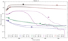 |
Fig. A.1 Dust mass accumulated over time around the Lagrangian points L4 (continuous line) and L5 (dotted line) for model 2. The evolution is shown for different sizes, including the effective (all sizes) accumulated mass (black continuous line). |
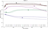 |
Fig. A.2 Dust mass accumulated in time around the Lagrangian points L4 (continuous line) and L5 (dotted line) for model 6. Evolution is shown for different sizes, including the effective (all sizes) accumulated mass (black continuous line). |
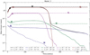 |
Fig. A.3 Dust mass accumulated over time around the Lagrangian points L4 (continuous line) and L5 (dotted line) for model 3. Evolution is shown for different sizes, including the effective (all sizes) accumulated mass. |
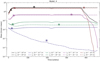 |
Fig. A.4 Dust mass accumulated over time around the Lagrangian points L4 (continuous line) and L5 (dotted line) for model 4. Evolution is shown for different sizes, including the effective (all sizes) accumulated mass. |
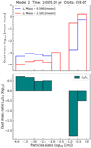 |
Fig. A.5 Mass spectrum of model 2 as a function of particle size for the dust accumulated in L4 and L5 for the last evolutionary stage (460 orbits). The bottom panel shows the mass ratio L4∕L5 as a function of particle size. |
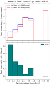 |
Fig. A.6 Mass spectrum of model 6 as a function of particle size for the dust accumulated in L4 and L5 for the last evolutionary stage (460 orbits). The bottom panel shows the mass ratio L4∕L5 as a function of particle size. |
References
- Andrews, S. M., & Williams, J. P. 2005, ApJ, 631, 1134 [NASA ADS] [CrossRef] [Google Scholar]
- Armitage, P. J. 2010, Astrophys. Planet Formation (Cambridge, UK: Cambridge University Press) [Google Scholar]
- Artymowicz, P. 1993, ApJ, 419, 155 [NASA ADS] [CrossRef] [Google Scholar]
- Bae, J., Zhu, Z., & Hartmann, L. 2016, ApJ, 819, 134 [NASA ADS] [CrossRef] [Google Scholar]
- Barge, P., & Sommeria, J. 1995, A&A, 295, L1 [NASA ADS] [Google Scholar]
- Baruteau, C., & Masset, F. 2008, ApJ, 678, 483 [NASA ADS] [CrossRef] [Google Scholar]
- Baruteau, C., & Zhu, Z. 2016, MNRAS, 458, 3927 [NASA ADS] [CrossRef] [Google Scholar]
- Baruteau, C., Barraza, M., Pérez, S., et al. 2019, MNRAS, 486, 304 [CrossRef] [Google Scholar]
- Beaugé, C., Sándor, Z., Érdi, B., & Süli, Á. 2007, A&A, 463, 359 [NASA ADS] [CrossRef] [EDP Sciences] [Google Scholar]
- Bouwman, J., de Koter, A., Dominik, C., & Waters, L. B. F. M. 2003, A&A, 401, 577 [NASA ADS] [CrossRef] [EDP Sciences] [Google Scholar]
- Brouwer, D., & Clemence, G. M. 1961, Orbits and Masses of Planets and Satellites, eds. G. P. Kuiper, & B. M. Middlehurst, 31 [Google Scholar]
- Chavanis, P. H. 2000, A&A, 356, 1089 [NASA ADS] [Google Scholar]
- Cresswell, P., & Nelson, R. P. 2009, A&A, 493, 1141 [NASA ADS] [CrossRef] [EDP Sciences] [Google Scholar]
- Crida, A., Baruteau, C., Kley, W., & Masset, F. 2009, A&A, 502, 679 [NASA ADS] [CrossRef] [EDP Sciences] [Google Scholar]
- Crnkovic-Rubsamen, I., Zhu, Z., & Stone, J. M. 2015, MNRAS, 450, 4285 [CrossRef] [Google Scholar]
- Cuello, N., Montesinos, M., Stammler, S. M., Louvet, F., & Cuadra, J. 2019, A&A, 622, A43 [NASA ADS] [CrossRef] [EDP Sciences] [Google Scholar]
- de Val-Borro, M., Edgar, R. G., Artymowicz, P., et al. 2006, MNRAS, 370, 529 [NASA ADS] [CrossRef] [Google Scholar]
- Desch, S. J. 2007, ApJ, 671, 878 [NASA ADS] [CrossRef] [Google Scholar]
- Di Sisto, R. P., Ramos, X. S., & Gallardo, T. 2019, Icarus, 319, 828 [NASA ADS] [CrossRef] [Google Scholar]
- Dohnanyi, J. S. 1969, J. Geophys. Res., 74, 2531 [NASA ADS] [CrossRef] [Google Scholar]
- Fitzsimmons, A., Dahlgren, M., Lagerkvist, C. I., Magnusson, P., & Williams, I. P. 1994, A&A, 282, 634 [Google Scholar]
- Flaherty, K., Hughes, A. M., Simon, J. B., et al. 2020, ApJ, 895, 109 [CrossRef] [Google Scholar]
- Freistetter, F. 2006, A&A, 453, 353 [NASA ADS] [CrossRef] [EDP Sciences] [Google Scholar]
- Fu, W., Li, H., Lubow, S., Li, S., & Liang, E. 2014, ApJ, 795, L39 [NASA ADS] [CrossRef] [Google Scholar]
- Gascheau, G. 1843, Compt. Rend. 16, 393 [Google Scholar]
- Giuppone, C. A., Benítez-Llambay, P., & Beaugé, C. 2012, MNRAS, 421, 356 [Google Scholar]
- Goldreich, P., & Tremaine, S. 1979, ApJ, 233, 857 [Google Scholar]
- Gomes, R. S. 1998, AJ, 116, 2590 [NASA ADS] [CrossRef] [Google Scholar]
- Hartmann, W. K., Tholen, D. J., Cruikshank, D. P., & Goguen, J. 1987, Meteoritics, 22, 399 [Google Scholar]
- Hildebrand, R. H. 1983, QJRAS, 24, 267 [NASA ADS] [Google Scholar]
- Isella, A., Benisty, M., Teague, R., et al. 2019, ApJ, 879, L25 [Google Scholar]
- Jedicke, R., Larsen, J., & Spahr, T. 2002, Observational Selection Effects in Asteroid Surveys, 71 [Google Scholar]
- Jewitt, D. C., Trujillo, C. A., & Luu, J. X. 2000, AJ, 120, 1140 [NASA ADS] [CrossRef] [Google Scholar]
- Kanagawa, K. D., Muto, T., Tanaka, H., et al. 2016, PASJ, 68, 43 [NASA ADS] [Google Scholar]
- Karlsson, O. 2010, A&A, 516, A22 [CrossRef] [EDP Sciences] [Google Scholar]
- Keppler, M., Benisty, M., Müller, A., et al. 2018, A&A, 617, A44 [NASA ADS] [CrossRef] [EDP Sciences] [Google Scholar]
- Klahr, H. H., & Bodenheimer, P. 2003, ApJ, 582, 869 [NASA ADS] [CrossRef] [Google Scholar]
- Klahr, H. H., & Lin, D. N. C. 2001, ApJ, 554, 1095 [NASA ADS] [CrossRef] [Google Scholar]
- Lagerkvist, C. I., Karlsson, O., Hahn, G., et al. 2002, Astron. Nachr., 323, 475 [CrossRef] [Google Scholar]
- Lagrange, J.-L. 1772, Oeuvres de Lagrange, 6, 229 [Google Scholar]
- Li, H., Finn, J. M., Lovelace, R. V. E., & Colgate, S. A. 2000, ApJ, 533, 1023 [NASA ADS] [CrossRef] [Google Scholar]
- Lillo-Box, J., Barrado, D., Figueira, P., et al. 2018a, A&A, 609, A96 [NASA ADS] [CrossRef] [EDP Sciences] [Google Scholar]
- Lillo-Box, J., Leleu, A., Parviainen, H., et al. 2018b, A&A, 618, A42 [NASA ADS] [CrossRef] [EDP Sciences] [Google Scholar]
- Lin, M.-K. 2012, MNRAS, 426, 3211 [NASA ADS] [CrossRef] [Google Scholar]
- Lovelace, R. V. E., Li, H., Colgate, S. A., & Nelson, A. F. 1999, ApJ, 513, 805 [NASA ADS] [CrossRef] [Google Scholar]
- Lyra, W., Johansen, A., Klahr, H., & Piskunov, N. 2009, A&A, 493, 1125 [NASA ADS] [CrossRef] [EDP Sciences] [Google Scholar]
- Masset, F. 2000, A&AS, 141, 165 [NASA ADS] [CrossRef] [EDP Sciences] [Google Scholar]
- Milani, A., Knežević, Z., Spoto, F., et al. 2017, Icarus, 288, 240 [NASA ADS] [CrossRef] [Google Scholar]
- Montesinos, M., Perez, S., Casassus, S., et al. 2016, ApJ, 823, L8 [NASA ADS] [CrossRef] [Google Scholar]
- Morbidelli, A., Levison, H. F., Tsiganis, K., & Gomes, R. 2005, Nature, 435, 462 [NASA ADS] [CrossRef] [PubMed] [Google Scholar]
- Murray, C. D. 1994, Icarus, 112, 465 [NASA ADS] [CrossRef] [Google Scholar]
- Nakamura, T.,& Yoshida, F. 2008, PASJ, 60, 293 [NASA ADS] [CrossRef] [Google Scholar]
- Paardekooper,S.-J. 2007, A&A, 462, 355 [NASA ADS] [CrossRef] [EDP Sciences] [Google Scholar]
- Pál, A., & Süli, Á. 2004, Publi. Astron. Depart. Eotvos Lorand Univ., 14, 285 [Google Scholar]
- Peale, S. J. 1993, Icarus, 106, 308 [NASA ADS] [CrossRef] [Google Scholar]
- Pinilla, P., Birnstiel, T., Ricci, L., et al. 2012, A&A, 538, A114 [NASA ADS] [CrossRef] [EDP Sciences] [Google Scholar]
- Pirani, S., Johansen, A., Bitsch, B., Mustill, A. J., & Turrini, D. 2019, A&A, 623, A169 [NASA ADS] [CrossRef] [EDP Sciences] [Google Scholar]
- Pitjeva, E. V., & Pitjev, N. P. 2020, Astron. Lett., 45, 855 [CrossRef] [Google Scholar]
- Raettig, N., Klahr, H., & Lyra, W. 2015, ApJ, 804, 35 [NASA ADS] [CrossRef] [Google Scholar]
- Semenov, D., Henning, T., Helling, C., Ilgner, M., & Sedlmayr, E. 2003, A&A, 410, 611 [NASA ADS] [CrossRef] [EDP Sciences] [Google Scholar]
- Shakura, N. I., & Sunyaev, R. A. 1973, A&A, 24, 337 [NASA ADS] [Google Scholar]
- Sheppard, S. S., & Trujillo, C. A. 2010, Science, 329, 1304 [NASA ADS] [CrossRef] [Google Scholar]
- Sosnitskii, S. 1996, J. Appl. Math. Mech., 60, 591 [CrossRef] [Google Scholar]
- Stammler, S. M. 2017, PhD thesis, Ruprecht Karl University of Heidelberg, https://www.imprs-hd.mpg.de/158403/thesis_stammler.pdf [Google Scholar]
- Surville, C., Mayer, L., & Lin, D. N. C. 2016, ApJ, 831, 82 [NASA ADS] [CrossRef] [Google Scholar]
- Szebehely, V. 1967, Theory of orbits. The Restricted Problem of Three Bodies [Google Scholar]
- Tatulli, E., Benisty, M., Ménard, F., et al. 2011, A&A, 531, A1 [NASA ADS] [CrossRef] [EDP Sciences] [Google Scholar]
- Tsiganis, K., Gomes, R., Morbidelli, A., & Levison, H. F. 2005, Nature, 435, 459 [NASA ADS] [CrossRef] [PubMed] [Google Scholar]
- Weidenschilling, S. J. 1977, MNRAS, 180, 57 [Google Scholar]
- Wolf, M. 1907, Astron. Nachr., 174, 1 [CrossRef] [Google Scholar]
- Yoshida, F., & Nakamura, T. 2005, AJ, 130, 2900 [NASA ADS] [CrossRef] [Google Scholar]
- Youdin, A. N., & Lithwick, Y. 2007, Icarus, 192, 588 [NASA ADS] [CrossRef] [Google Scholar]
- Zhang, S., Zhu, Z., Huang, J., et al. 2018, ApJ, 869, L47 [NASA ADS] [CrossRef] [Google Scholar]
- Zsom, A., Sándor, Z., & Dullemond, C. P. 2011, A&A, 527, A10 [NASA ADS] [CrossRef] [EDP Sciences] [Google Scholar]
Available data on protoplanetary disks suggest α ~ 10−4, e.g., Zhang et al. (2018); Flaherty et al. (2020).
The Hill radius is defined  , where
rp is the star–planet distance (the planet has no eccentricity in our models), Mp the mass of the planet, and M⋆ the mass of the star. We adopt RCPD = 0.6Rhill which is a suitable choice for Jupiter-like planets around a solar mass star (Crida et al. 2009).
, where
rp is the star–planet distance (the planet has no eccentricity in our models), Mp the mass of the planet, and M⋆ the mass of the star. We adopt RCPD = 0.6Rhill which is a suitable choice for Jupiter-like planets around a solar mass star (Crida et al. 2009).
All Tables
Dust properties at the Lagrangian points L4 and L5 computed forthe last evolutionary stage (460 orbits).
All Figures
|
Fig. 1 Equipotential lines according to Eq. (11) in a rotating frame with the planet, applied to a model with parameters M⋆ = 1 M⊙, rp = 7.8 au, and Mp = 5 MJ. The leading Lagrangian point (L4) is located at + π∕3, while the trailing point (L5) is at − π∕3. A stable librating azimuthal angle is assumed to be ±π∕8 around eachLagrangian point. |
| In the text | |
|
Fig. 2 Evolution of the gas and dust in model (1), for three evolutionary stages; 46, 230, and 459 orbits. The dust panels show the full size range of the particles, from 10−4 to 100 cm. The panels have been rotated to always keep the planet at the same location x = 7.8 au, y = 0. |
| In the text | |
|
Fig. 3 Top: Evolution of the vortensity and dust in model 1, for three evolutionary stages: 46, 230, and 459 orbits. Bottom: Dust distribution of particles with sizes in the range 10−2 − 100 cm. The planet rotates in the counter-clockwise direction. The panels have been rotated to always keep the planet at the same location, namely x = 7.8 au, y = 0. |
| In the text | |
|
Fig. 4 Evolution in time of the dust for model 1 as a function of particle size, ranging from μm to cm. The panels have been rotated to always keep the planet at the same location x = 7.8 au, y = 0. |
| In the text | |
|
Fig. 5 Mass spectrum of model 1 as a function of the size of the dust accumulated in L4 and L5 for thelast evolutionary stage (460 orbits). The bottom panel shows the mass ratio L4 ∕L5 as a function of dust particle size. |
| In the text | |
|
Fig. 6 Mass spectrum of model 1 as a function of the Stokes number for the dust accumulated in L4 and L5 at the last evolutionary stage (460 orbits). The bottom panel shows the mass ratio L4∕L5. |
| In the text | |
|
Fig. 7 Histogram of the effective dust mass accumulated at the end of the simulation inside L4 and L5, distributed by radial bins. This defines a capture region given by rp + 2RHill from the planet towards the outer region, and rp − 1.5RHill from the planet towards the star. An effective capture radius is expected at rp ± Rhill. |
| In the text | |
|
Fig. 8 Dust mass accumulated in time around the Lagrangian points L4 (continuous line) and L5 (dotted line) for model 1. The evolution is shown for different sizes, including the effective (all sizes) accumulated mass (black continuous line). |
| In the text | |
|
Fig. 9 Radial trajectory of randomly selected particles (μm to cm) that end up trapped in the second inner ring located at r = 5.6 au featured at the end of the simulation in model 1. |
| In the text | |
|
Fig. 10 Trajectories of some particles (μm to cm) from model 1 that end up trapped inside the Lagrangian point L4 only. The top horizontal red lines represent the location L5, while the bottom horizontal lines represent L4. Some submm particles oscillate in horseshoe orbits (between both L4 and L5) before ending in L4. Large mm–cm particles oscillate only in tadpole orbits around L4. |
| In the text | |
|
Fig. 11 Radial trajectory of randomly selected particles (μm to cm) that end up trapped in the outer ring located at r = 11 au featured at the end of the simulation model 1. |
| In the text | |
|
Fig. 12 Spectral energy distribution from the disk, and the Lagrangian point L5 from model 1 computed at the last evolutionary stage. Emission from the Lagrangian point comes from an optically thin dusty swarmof ~3 Mmoon with a mean temperature of ~55 K. |
| In the text | |
|
Fig. A.1 Dust mass accumulated over time around the Lagrangian points L4 (continuous line) and L5 (dotted line) for model 2. The evolution is shown for different sizes, including the effective (all sizes) accumulated mass (black continuous line). |
| In the text | |
|
Fig. A.2 Dust mass accumulated in time around the Lagrangian points L4 (continuous line) and L5 (dotted line) for model 6. Evolution is shown for different sizes, including the effective (all sizes) accumulated mass (black continuous line). |
| In the text | |
|
Fig. A.3 Dust mass accumulated over time around the Lagrangian points L4 (continuous line) and L5 (dotted line) for model 3. Evolution is shown for different sizes, including the effective (all sizes) accumulated mass. |
| In the text | |
|
Fig. A.4 Dust mass accumulated over time around the Lagrangian points L4 (continuous line) and L5 (dotted line) for model 4. Evolution is shown for different sizes, including the effective (all sizes) accumulated mass. |
| In the text | |
|
Fig. A.5 Mass spectrum of model 2 as a function of particle size for the dust accumulated in L4 and L5 for the last evolutionary stage (460 orbits). The bottom panel shows the mass ratio L4∕L5 as a function of particle size. |
| In the text | |
|
Fig. A.6 Mass spectrum of model 6 as a function of particle size for the dust accumulated in L4 and L5 for the last evolutionary stage (460 orbits). The bottom panel shows the mass ratio L4∕L5 as a function of particle size. |
| In the text | |
Current usage metrics show cumulative count of Article Views (full-text article views including HTML views, PDF and ePub downloads, according to the available data) and Abstracts Views on Vision4Press platform.
Data correspond to usage on the plateform after 2015. The current usage metrics is available 48-96 hours after online publication and is updated daily on week days.
Initial download of the metrics may take a while.