| Issue |
A&A
Volume 642, October 2020
|
|
|---|---|---|
| Article Number | A69 | |
| Number of page(s) | 10 | |
| Section | Extragalactic astronomy | |
| DOI | https://doi.org/10.1051/0004-6361/202038725 | |
| Published online | 06 October 2020 | |
The different flavors of extragalactic jets: The role of relativistic flow deceleration
1
INAF/Osservatorio Astrofisico di Torino, Via Osservatorio 20, 10025 Pino Torinese, Italy
e-mail: This email address is being protected from spambots. You need JavaScript enabled to view it.
2
Dipartimento di Fisica, Università degli Studi di Torino, Via Pietro Giuria 1, 10125 Torino, Italy
Received:
23
June
2020
Accepted:
22
July
2020
Abstract
We perform three-dimensional numerical simulations of relativistic (with a Lorentz factor of 10), non-magnetized jets propagating in a uniform density environment in order to study the effect of the entrainment and the consequent deceleration. Our simulations investigate the jet propagation inside the galaxy core, where the deceleration most likely occurs more efficiently. We compare cases with different density and pressure ratios with respect to the ambient medium and find that low density jets are efficiently decelerated and reach a quasi-steady state in which, over a length of 600 jet radii, they slow down from highly relativistic to sub-relativistic velocities. Conversely, denser jets keep highly relativistic velocities over the same length. We discuss these results in relation to the Faranoff Riley (FR) radio source classification. We infer that lower density jets can give rise to FR 0 and FR I radio sources, while higher density jets may be connected to FR II radio sources.
Key words: hydrodynamics / methods: numerical / galaxies: jets
© ESO 2020
1. Introduction
Extragalactic radio sources are traditionally divided into two morphological classes according to their intrinsic radiative power (Fanaroff & Riley 1974): low luminosity sources (Fanaroff-Riley type I, or FR I) are brighter close to the nucleus of the parent galaxy and their jets become dimmer with distance, while high power sources (Fanaroff-Riley type II, or FR II) show the maximum brightness in the hot spots at the jet termination. The different morphology is generally accepted as reflecting a difference in how the jet energy is dissipated during propagation in the ambient medium. In FR II sources, energy and momentum are transported without strong losses to the jet termination, while turbulence and entrainment must play an important role in shaping FR I source morphology. Recently, a third class has been introduced by Baldi et al. (2015) and is referred to as FR 0. The sources belonging to this type are highly core dominated and generally do not present the prominent extended radio structures typical of FR I and FR II sources. Nonetheless, evidence for small-scale jets (limited to sizes of a few kpc) are found in a minority of FR 0 sources (Baldi et al. 2019). This suggests that their jets are not even able to escape from the galaxy core.
Observational evidence shows that, both in FR II and in FR I sources, the jets at their base (at the parsec scale) are relativistic, with very similar Lorentz factors (Giovannini et al. 2001; Celotti & Ghisellini 2008). Massaro et al. (2020) find that the FR 0 represents the misaligned counterparts of a significant fraction of BL Lac objects; BL Lacs are known to be associated with highly relativistic jets (Blandford & Rees 1978) and this result implies that at least some FR 0 sources must also launch relativistic outflows. It is then clear that in FR I jets a deceleration to sub-relativistic velocities must occur between the inner region and the kiloparsec scale, where they show their typical plume-like, turbulent morphology (Laing & Bridle 2002, 2014). The same effect must occur also in FR 0 at even smaller distances from the jet origin. Assuming that the deceleration to a sub-relativistic velocity occurred inside the galaxy core, Massaglia et al. (2016, hereinafter Mas16) performed high-resolution three-dimensional Newtonian simulations of low Mach number jets, showing how turbulence develops and gives rise to a jet structure very similar to that observed in FR I sources. Recently van der Westhuizen et al. (2019), using injection parameters similar to those of Mas16 and applying a recipe for the synchrotron radiation investigated whether the emission map could be comparable to FR I observations.
A very likely mechanism through which deceleration occurs is the entrainment of material from the ambient medium (De Young 1993, 2005; Bicknell 1984, 1986, 1994), promoted by different kinds of jet instabilities (see, e.g., Perucho et al. 2005, 2010; Perucho & Martí 2007; Meliani & Keppens 2007, 2009; Bodo et al. 2013; Matsumoto & Masada 2013; Millas et al. 2017; Toma et al. 2017; Gourgouliatos & Komissarov 2018a; Tchekhovskoy & Bromberg 2016; Mukherjee et al. 2020). Another possibility suggested by Komissarov (1994) is mass loading by stellar winds; this approach has since been investigated by Bowman et al. (1996), Hubbard & Blackman (2006), Perucho et al. (2014). More recently Perucho (2020) suggests that stars may trigger mixing by generating small-scale instabilities.
Since FR I jets are less powerful than FR II jets, but have similar Lorentz factors, they have to be less dense and therefore more prone to deceleration by the external medium. Rossi et al. (2008) performed numerical simulations of the propagation of relativistic jets with different values of the density ratio between the jet and the ambient medium; they showed that, while jets with density ratios between 0.01 and 0.1 (and power corresponding to FR II) propagate almost undisturbed, jets with lower values of the density ratio (and power corresponding to FR I) show evidence of entrainment and deceleration in their external layers. Due to the limitations of computational power, Rossi et al. (2008) could only follow the jet propagation up to about 60 jet radii and could not see a complete transition to sub-relativistic velocities; in fact, the jet core remained relativistic in their simulations.
In this paper we extend the Rossi et al. (2008) study by following the jet propagation up to 600 jet radii, a distance that, assuming an initial jet radius on the order of 1 pc, covers the full galaxy core. We consider similar jet parameters and the corresponding jet powers are at or below the FR I–FR II transition value. In Sect. 2 we describe the set of equations to be solved, the numerical method, the initial and boundary conditions, and the parameters of the simulations. In Sect. 3 we present our results and in Sect. 4 we give a discussion and conclusions.
2. Numerical setup
Numerical simulations were carried out by solving the equations of particle number and energy-momentum conservation. Referring to the observer’s reference frame, where the fluid moves with velocity vk (in units of the speed of light c) with respect to the coordinate axes k = x, y, z and assuming a flat metric, the conservation laws take the differential form:
 (1)
(1)
where ρ, w, p, and γ denote the rest mass density, enthalpy, gas pressure, and Lorentz factor, respectively. The jet and external material were distinguished by using a passive tracer, f, set equal to unity for the injected jet material and equal to zero for the ambient medium. We took the jet radius as the unit of length, the speed of light as the unit of velocity, and the light crossing time of the jet radius as the unit of time. The system of Eq. (1) was completed by specifying an equation of state relating w, ρ, and p. Following Mignone et al. (2005), we adopted the Taub-Matthews (TM) equation of state with the prescription:
 (2)
(2)
which closely reproduces the thermodynamics of the Synge gas for a single-species relativistic perfect fluid.
Simulations were carried out on a Cartesian domain with coordinates in the range x ∈ [ − Lx/2, Lx/2], y ∈ [0, Ly], and z ∈ [ − Lz/2, Lz/2] (lengths are expressed in units of the jet radius). At t = 0, the domain was filled with a perfect fluid of uniform density and pressure, representing the external ambient medium initially at rest. The assumption of constant external density is consistent with the fact that we focused on the jet propagation inside the galaxy core.
A cylindrical inflow of velocity vj was constantly fed into the domain through the lower y boundary along y direction. The jet is characterized by the Lorentz factor γj, by the ratio K between the proper (pj) and ambient (p0) pressures, and the ratio η between the proper (ρj) and ambient (ρ0) densities. The jet Mach number can be derived using the expression of the sound speed for the TM equation of state (Mignone et al. 2005):
 (3)
(3)
The classical Mach number is defined as M = vj/cs; in the relativistic case, we can define a generalization (Königl 1980) as Mr = γjvj/γscs, where  . Outside the inlet region, we imposed symmetric boundary conditions (emulating a counter-jet), whereas the flow can freely leave the domain through the remaining boundaries.
Explicit numerical integration of the Eq. (1) was achieved using the relativistic hydrodynamics module available in the PLUTO code (Mignone et al. 2007). For the present application, we employed linear reconstruction and the HLLC Riemann solver (Mignone & Bodo 2005). The physical domain was covered by Nx × Ny × Nz computational zones, which were not necessarily uniformly spaced. For domains with a large physical size, we employed a uniform grid resolution around the beam (typically for |x|,|z| ≤ 7) and a geometrically stretched grid elsewhere.
We performed a set of four simulations, whose parameters are reported in Table 1. All the cases have the Lorentz factor γj = 10; cases A, B, and D differ by the density ratios η, which are, 10−3, 10−4, and 10−2 respectively, while cases B and C have the same density ratio and differ by the pressure ratio K.
Parameter set used in the numerical simulation model.
3. Results
Our aim is to understand how the deceleration of a relativistic jet depends on its physical parameters. In principle, the setup of our simulations is such that the results are scale invariant; however, our interest is focused on the deceleration that mainly occurs in the first kiloparsec. This motivates our assumption of constant density of the external medium because the domain of our simulations can be assumed to be all contained within the galaxy core. We can then adopt a jet injection radius on the order of one parsec and the external density at injection on the order of one particle per cubic centimeter (Balmaverde et al. 2008).
In the following we will express all quantities in their non-dimensional values as defined in the previous section. Conversion to physical units can be obtained with the above assumptions; in particular, the unit of time is
 (4)
(4)
and the jet power is
 (5)
(5)
where h is the specific enthalpy and n0 is the external number density at the injection point. The jet power for the four cases (with specific enthalpy h = 1.2, 1.2, 3.45, and 1.2 for cases A to D respectively) are reported in Table 1. We chose the jet parameters so that the resulting powers span an interval between FR I and FR II. Case D can be taken as a reference case, as it is clearly on the FR II side.
We follow the jet propagation until the bow shock in front reaches y = 600; the lateral extension of the domain is such that the entire bow shock is included in the computational domain. In Fig. 1, we display the whole computational domain showing a longitudinal cut (in the y − z plane) of the distribution of the logarithm of the pressure for case C at the end of the simulation. The two dashed yellow lines indicate the central region on which we will focus in the following analysis.
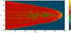 |
Fig. 1. Longitudinal cut (in the y − z plane) of the distribution of the logarithm of the pressure for case C at t = 11 500 when the bow shock in front of the jet reaches y = 580. The image shows the whole computational domain. The two dashed yellow lines indicate the central region on which we will focus in the following analysis. |
In Figs. 2–4, we show the jet structure for the first three cases, when the bow shock in front of the jet reaches 600 length units. These three snapshots correspond to three different times, namely t = 6000 for case A, t = 25 000 for case B and t = 12 500 for case C; the differences in times are due to the different jet head propagation velocities, as we will see below. In the figures, we display three- dimensional views of the isocontours for three values of the Lorentz gamma factor. In the top panel of each figure, we have the entire jet, and in the bottom panel we zoom in on the last 200 length units. The represented domain, in the transverse section, spans from −30 to 30 in both directions. In all the three cases, we can see that there is a first region (up to y ∼ 150 − 250) in which the jet seems to propagate straight, although, as we will see below, perturbations are already present and growing. Then we observe perturbations that lead to a displacement of the jet axis. Finally, in the last part of the jet, we see that the fast-moving material fragments (see bottom panels), and we have a wide low-velocity envelope in which a few blobs still move at high γ.
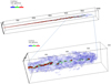 |
Fig. 2. Three-dimensional isosurfaces of the Lorentz factor for case A. Top panel: entire jet, while bottom panel: last portion between y = 400 and y = 600. The snapshot is taken at t = 6000 when the jet head reaches y ∼ 600. The three isosurfaces are for γ = 1.5, 3, 5 in the top panel and γ = 1.1, 3, 5 in the bottom panel. |
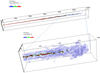 |
Fig. 3. Three-dimensional isosurfaces of the Lorentz factor for case B. Top panel: entire jet, while bottom panel: last portion between y = 400 and y = 600. The snapshot is taken at t = 25 000 when the jet head reaches y ∼ 600. The three isosurfaces are for γ = 1.5, 3, 5 in the top panel and γ = 1.1, 3, 5 in the bottom panel. |
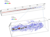 |
Fig. 4. Three-dimensional isosurfaces of the Lorentz factor for case C. Top panel: entire jet, while bottom panel: last portion between y = 400 and y = 600. The snapshot is taken at t = 12 500 when the jet head reaches y ∼ 600. The three isosurfaces are for γ = 1.5, 3, 5 in the top panel and γ = 1.1, 3, 5 in the bottom panel. |
In order to better understand the jet evolution outlined above, we will discuss case B in more detail; in Fig. 5 we display a longitudinal cut (in the y − z plane) of the distribution of the Lorentz factor at t = 25 000 when the jet head reaches y = 600. We highlight the three regions of different jet behavior with different colors. In the first region (up to y ∼ 250, region I), we see a series of recollimation shocks that modulate the jet radius. Starting from the second recollimation shock, we notice the formation and growing of perturbations, leading, in region II, to a displacement of the jet from its original axis and to entrainment of slow-moving material. Finally, in the last region, the jet is broken into a few fast-moving blobs surrounded by a wide low-velocity envelope (region III).
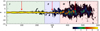 |
Fig. 5. Longitudinal cut (in the y − z plane) of the distribution of the Lorentz factor for case B at t = 25 000 when the jet head reaches y = 600. The three colored bands highlight the three phases described in the text. The red arrows mark the positions at which the transverse cuts shown in Fig. 6 are taken. |
In Fig. 6, we show three transverse (in the x − z plane) cuts of the distribution of the γ factor; their positions are indicated with red arrows in Fig. 5. The three panels show different stages of the evolution of the perturbations: (1) at the beginning the jet cross section is slightly deformed; (2) it then becomes completely distorted; (3) in the last panel, it appears to be more spread out and the maximum value of the Lorentz factor is reduced to γ = 5. The last x − z cut is through a fast-moving blob; in other positions the maximum γ is ≈2.
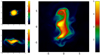 |
Fig. 6. Transverse cuts (in the x − z plane) of the distribution of the Lorentz factor at three different positions along the jet for case B at t = 25 000 when the jet head reaches y = 600. The positions of the three cuts correspond to the three red arrows in Fig. 5. Top-left panel: y = 100, the bottom-left panel is at y = 300, and the right panel is at y = 450. We remark that the two left panels cover a square with −4 ≤ x, z ≤ 4, while the right panel covers −8 ≤ x, z ≤ 8; moreover, in the two left panels, the maximum γ is 10, while in the right panel the maximum γ is 5. |
The other two cases (A and C) also show a similar behavior, which we can analyze by looking at Fig. 7; here we plot the maximum distance from the jet axis, at which we still find jet material moving with γ ≥ 5. In the figure, we identify the three defined regions, whose lengths and starting points are different for the three cases, with different colors. For case A (left panel) we observe that perturbations start to form and grow at y = 50, and that from y = 250 they induce jet oscillation. At y = 450, the jet breaks and, in fact, we see intervals in which there is no jet material with γ ≥ 5. In the middle panel, we present case B, which displays the characteristics we talked about when discussing Fig. 5. In particular, we highlight the modulation of the jet radius by recollimation shocks (between y = 0 and y = 200), the growing of perturbations (region II), and the final jet disruption. In case C (right panel), we see a sudden expansion, due to the fact that the jet is overpressured, modulated by recollimation shocks up to y = 150; then perturbations grow and lead to smaller-amplitude oscillations with respect to case A. The jet breaking occurs at y > 350.
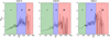 |
Fig. 7. Maximum distance from the initial jet axis at which we find material moving at γ ≥ 5 as a function of y. The three panels refer to the three cases; the times are, respectively, t = 6000, 12 500, and 25 000 when the jet head reaches y = 600. The three colored bands highlight the three phases described in the text. |
The results presented above show that the jet progressively decelerates and the quantity of material moving at high γ decreases, while an increasing amount of material around the jet moves at γ ≤ 2.
Now we can analyze more quantitatively how the deceleration occurs or, in other words, how the jet transfers its momentum to the external medium. In Fig. 8, we plot, as a function of time, the maximum distance at which a given fraction of the momentum flux is carried by material moving at γ ≥ 5. For example, looking at the left panel (case A), we have eight curves enclosing seven colored regions. Starting from the top: the thick black curve represents the head position; the first region refers to a jet section in which the high-velocity material carries a fraction of momentum flux ≤10%; the second band refers to a fraction 10%−20% and so on; the bottom curve refers to a fraction of 70%. Up to t ≈ 2000, all the curves follow the behavior of the jet head, and all the momentum transfer occurs close to the terminal shock. Subsequently, the curves, starting from the bottom progressively flatten. The flattening of the curves indicates that the jet has reached a quasi steady-state up to that position; for example the 70% curve (the lowest one) flattens at y ≈ 250. This means that the fast-moving material, up to that point, loses in a steady way 30% of its momentum flux; in other words, 70% of the momentum flux of the fast-moving material goes beyond y ≈ 250, and this fraction remains constant in time. Between y = 250 and y = 450, the jet material moving at γ ≥ 5 carries a fraction of momentum flux, decreasing from 70% to about 30%. The 10% and 20% curves still stay parallel to the head position curves. The last portion of the jet has not yet reached a steady configuration and the remaining ∼30% of momentum is transferred in the region close to the terminal shock. Case B shows a similar behavior; however the flattening of the curves starts at an earlier time. Moreover, the 20% and 10% curves also show a more pronounced change of slope. Case C has a non-monotonic behavior and will be discussed in more detail below.
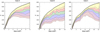 |
Fig. 8. Maximum distance from the jet origin at which a given fraction of momentum flux is carried by material moving at γ ≥ 5 as a function of time. From the top: jet head position (black thick curve); and the curves from 10% to 70% in blocks of 10%. We highlight the areas between subsequent curves with different colors. |
In Fig. 9, we give for case B a different view of the same distribution shown in Fig. 8. We plot two vertical cuts from middle panel of Fig. 8 at two different times, that show the fraction of momentum flux carried by high-velocity material (γ ≥ 5) as a function of y. The curve at the later time (red curve) is shifted by few tens of length units, while the jet head, in the same time interval, advanced from y ∼ 400 to y ∼ 600, indicating the quasi-steady state reached by the jet, as previously discussed. Furthermore, as stressed before, the high-velocity material appears to be fragmented in the front part of the jet.
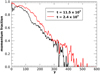 |
Fig. 9. Fraction of momentum flux carried by material moving at γ ≥ 5 as a function of y at two different times, for case B. |
Combining the information obtained from Figs. 7–9, we derive a scenario in which the jet, as a result of instabilities, releases its momentum progressively and in a quasi steady way into the surrounding material;it widens its cross section maintaining a high gamma value only in a central spine until it breaks and fragments into high-velocity blobs, surrounded by an envelope at γ ≤ 2. We can see that all the three cases (A, B, and C) show a quasi steady state up to y ≈ 400 − 500; however, they differ in the fraction of momentum flux lost by the high-velocity material, that is about 70% for case A and about 90% for cases B and C. It may be interesting, at this point, to discuss the differences between cases B and C. At the end of the simulations, when the head reaches y = 600, they present a similar distribution of the transfer of momentum flux; however, the evolution is quite different at earlier times. In case B the momentum curves flatten quite early, while in case C they show an irregular behavior, reach a maximum, and then move back toward the jet origin. The two cases have the same density ratio and differ in the pressure ratio, with case C being overpressured. Case C then carries higher energy and momentum fluxes. Moreover, in the first part of the simulation, the cocoon is overpressured with respect to the jet for all cases, and drives recollimation shocks into the jet, which are stronger in cases B and C. Then, as the cocoon expands, its pressure decreases and, for case C, becomes on the order of the jet pressure; the recollimation shocks then become weak or disappear entirely. Finally, when the cocoon pressure becomes much lower than the jet pressure, the jet expands and recollimates, again in a series of shocks. This behavior appears to be correlated with the behavior of the curves of the transfer of momentum flux, which reflect the position at which the instabilities have a substantial growth. This connection between recollimation shocks and the starting of instabilities could be related to the recent results by Gourgouliatos & Komissarov (2018a,b), who discuss a centrifugally driven instability of such structures; however higher-resolution simulations would be needed to make a more precise statement.
The spreading of momentum discussed above leads to a decrease in the strength of the terminal shock up to its disappearance. in Mas16 the authors interpret this disappearance as a signature of the transition from FR II to FR I; in fact the presence of a strong terminal shock can be connected with the presence of hot spots typical of FR II radio sources. In Fig. 10, we plot the maximum pressure on a transverse x − z plane at a given position y along the jet, as a function of y. The two curves in each panel refer to two different (but very close) times, when the jet has reached its maximum extension. The peaks close to the jet origin are related to the recollimation shocks, which, as we previously pointed out, are progressively dissolved by the instability; they are more evident in cases B and C. In all the cases, the black curve presents a strong terminal shock, which is not present in the red curve. This demonstrates the highly inhomogeneous jet structure discussed above: The strong shock is related to one of the high-velocity blob reaching the head.
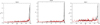 |
Fig. 10. Maximum pressure on a transverse x − z plane at a given position y along the jet as a function of y. The red and black curves in each panel refer to two different (but very close) times, when the jet reaches its maximum extension. |
Figure 11 represents the maximum pressure in the computational domain, which in general corresponds to the pressure of the terminal shock as a function of the head position. In Figs. 11 and 12, we chose to do the plots as a function of the jet head position instead of time, to facilitate comparison between the cases. Figure 11 clearly shows that this quantity is highly fluctuating; for this reason, we highlighted the variability range with colored bands. All three cases show a general decrease in the maximum pressure at the terminal shock, which can be correlated with a deceleration of the head velocity toward low Mach numbers. This deceleration is confirmed by Fig. 12, in which we plot the head Mach number relative to the external sound speed as a function of head position. We note how this number approaches unity (M = 3 − 4) for cases B and C but remains larger for case A (M = 10 − 20). Moreover, while the curve for case A is smooth and starts to present oscillations only in the last part, the wiggling portion widens for case C; for case B, the head velocity is highly variable from the beginning. This indicates that the fragmentation of the jet occurs earlier in time for case B and progressively later for cases C and A, and may be related to a stronger entrainment and mixing for case B in comparison to cases C and A. Indeed, the width of the variation of the maximum pressure plotted in Fig. 11 is larger for case B. In the same figure we also plot the head Mach number for case D (black curve). For this last case we see very little deceleration: The Mach number decreases from ∼200 to slightly less than 100.
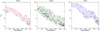 |
Fig. 11. Maximum pressure found in the computational domain as a function of the position reached by the jet head. The symbols mark the values for each time, while the colored band identifies the range of variation. The three cases have different numbers of point values due to the different jet head velocities: A lower velocity (case B) implies a larger number of marks. |
Now, we discuss separately case D, which has a higher density ratio (η = 10−2) and therefore a larger jet power. On the basis of the results presented so far, we can expect a much less efficient deceleration, and, indeed, Fig. 12 confirms this expectation. A weaker interaction with the ambient medium is demonstrated by Fig. 13, where we show a longitudinal cut (in the y − z plane) of the distribution of the γ factor. As we have done previously, we identify three separate regions: the first one, in which the jet propagates straight, extends up to y ∼ 320, far beyond the other cases; the second one, in which the instability leads to a jet deformation, covers almost completely the remaining portion of the jet. The third one is practically absent, and, in fact, the jet fragmentation occurs only at its head. As a result we see that material moving at γ > 8 almost continuously reaches the jet front. Further confirmation comes from Fig. 14, where, similarly to Fig. 8, we plot, as a function of time, the maximum distance at which a given fraction of the momentum flux is carried by material moving at γ ≥ 5. Differently from the other cases presented in Fig. 8 all the curves grow with the same slope as the one related to the jet head position, indicating that no steady state has been reached and that all the momentum transfer always happens at the jet head. We can conclude that heavier and more powerful jets cannot be efficiently decelerated within the galaxy core region.
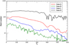 |
Fig. 12. Jet head Mach number, relative to the ambient medium, as a function of the head position. The three curves refer to the three cases. |
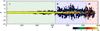 |
Fig. 13. Longitudinal cut (in the y − z plane) of the distribution of the Lorentz factor for case D at t = 1300 when the jet head reaches y = 600. The three colored bands highlight the three phases described in the text. |
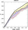 |
Fig. 14. Maximum distance from the jet origin at which a given fraction of momentum flux is carried by material moving at γ ≥ 5 as a function of time. From the top: jet head position and the curves from 10% to 70% in blocks of 10%. We highlight the areas between subsequent curves with different colors. |
As an aside, we remark that our results confirm that the assumptions in Mas16 are roughly consistent with the results achieved in this paper. In Figs. 15 and 16 we show a typical distribution of the Mach number and of the density in the terminal part of the jet. The maximum Mach number is ∼2, with a corresponding density of ∼10−2, while in the surrounding region the density is ∼10−1. This demonstrates a strong mixing with the external medium, considering that the injected jet density was 10−4. We notice that our results are consistent with the model by Bicknell (1995), who estimated that flows decelerating to sub-relativistic velocities acquire a Mach number on the order of 2.
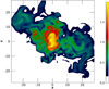 |
Fig. 15. Transverse cut (in the x − z plane) of the Mach number for case B at y = 450 and t = 25 000. |
4. Discussion and conclusions
We presented three-dimensional simulations of relativistic jets, considering four cases with the same Lorentz factor γ = 10 but with different density and pressure ratios and, correspondingly, different powers. These results can be interpreted in relation to the FR I–FR II classification; assuming a jet injection radius on the order of one parsec, the powers span an interval between the two classes. Case D can be taken as a reference case, being clearly on the FR II side. We follow the propagation up to 600 pc, within the galaxy core, so our assumption of constant density is well justified. In Mas16 the authors, by performing Newtonian simulations, showed that low power jets give rise to a turbulent morphology typical of FRI radio sources, and they give constraints on the physical parameters at the injection point for obtaining such morphology. In this respect, our simulations aim at answering the following two questions: Knowing that FR I jets are relativistic at their base, can they decelerate to sub-relativistic velocity within the first kiloparsec? Are the jet parameters obtained at the distance of about one kiloparsec comparable to the injection parameters assumed in Mas16?
Our results show that relativistic jet deceleration occurs as the consequence of instabilities, which in their growth progressively deform the jet, induce mixing and transfer of momentum to the ambient medium, and finally lead to a fragmentation of the jet itself. However, other important questions arise: does the deceleration process described above occurs in a quasi-steady way or the jet is capable of reestablishing itself and does the deceleration length increase as the jet pierces its way through the ambient medium? We show evidence that indeed, during the time span of our simulations, a quasi-steady state is reached at least up to ∼500 pc. Nevertheless, cases A, B, and C differ in the fraction of momentum transferred (by high-velocity material) to the ambient: 90% for cases B and C, and on the order of 70% for case A. In all three cases, the resulting jet structure, at the end of the steady state region, is a broad flow, moving at about γ ≤ 2, interspersed by blobs at γ ≥ 5. Extrapolating these results, if we increase η, and, consequently, the jet power, the length of the steady deceleration region will likely increase and the transferred fraction of momentum will decrease; indeed, case D with η = 10−2 does not show any deceleration effect. Therefore, if the jet does not decelerate inside the galaxy core it is unlikely that the deceleration will happen in the intergalactic medium with its declining density. On the other hand, decreasing η, we expect an increase in the transferred momentum fraction with a consequent stronger deceleration. In this respect, we can speculate that jets with very low η could be not able to propagate much farther than the galaxy core, and could be connected to FR 0 radio sources. Cases A, B, and C seem to represent limiting cases for which an effective deceleration may occur inside the galaxy core. The important role played by the density ratio, in the instability evolution and in the mixing andentrainment process, has previously been investigated both considering jet propagation and more idealized settings (see, e.g., Bodo et al. 1995; Perucho et al. 2004, 2005; Rossi et al. 2008), and our present results confirm their findings. The role of instabilities on the jet dynamics, at much larger scales, has recently been investigated by Perucho et al. (2019) and Mukherjee et al. (2020), who showed that instabilities may lead to some deceleration at larger scales in higher power jets as well.
Furthermore, we can confirm that the Mas16 assumptions regarding the jet injection parameters are roughly consistent with the results achieved in this paper, as shown in Figs. 15 and 16 which display typical distributions of the Mach number and of the density in the terminal part of the jet. Clearly the assumption, used in Mas16, of a spatially and temporally homogeneous flow is very simplified; our results show that there are intervals of time in which high-velocity confined structures may still be present; this behavior could provide a perspective on further investigations, along the line of Mas16, in which these inhomogeneities can be taken into account.
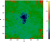 |
Fig. 16. Transverse cut (in the x − z plane) of the density for case B at y = 450 and t = 25 000. |
Our simulations consider a homogeneous external medium; the presence of strong inhomogeneities could have an impact on the jet dynamics, as shown by Mukherjee et al. (2016), possibly enhancing the entrainment effect. Finally, the presence of a magnetic field introduces new kinds of instabilities whose importance depends on the field strength and configuration (Bodo et al. 2013). A strong toroidal component could on one hand lead to a stabilization of velocity shear instabilities, which play a major role in the present case, but at the same time introduce current driven instabilities that may also lead to a jet deceleration (Mignone et al. 2010; Tchekhovskoy & Bromberg 2016; Massaglia et al. 2019; Mukherjee et al. 2020). On the other hand, with a weaker and more longitudinal field, velocity shear instabilities may still be the dominant ones.
Acknowledgments
We thank Manel Perucho for the helpfull comments. We acknowledge support by the Accordo Quadro INAF-CINECA 2017 for the availability of high performance computing resources. We acknowledge also support from PRIN MIUR 2015 (grant number 2015L5EE2Y). Calculations have been carried out at the CINECA and at the Competence Centre for Scientific Computing (C3S) of the University of Torino.
References
- Baldi, R. D., Capetti, A., & Giovannini, G. 2015, A&A, 576, A38 [NASA ADS] [CrossRef] [EDP Sciences] [Google Scholar]
- Baldi, R. D., Capetti, A., & Giovannini, G. 2019, MNRAS, 482, 2294 [NASA ADS] [CrossRef] [Google Scholar]
- Balmaverde, B., Baldi, R. D., & Capetti, A. 2008, A&A, 486, 119 [NASA ADS] [CrossRef] [EDP Sciences] [Google Scholar]
- Bicknell, G. V. 1984, ApJ, 286, 68 [NASA ADS] [CrossRef] [Google Scholar]
- Bicknell, G. V. 1986, ApJ, 300, 591 [NASA ADS] [CrossRef] [Google Scholar]
- Bicknell, G. V. 1994, ApJ, 422, 542 [NASA ADS] [CrossRef] [Google Scholar]
- Bicknell, G. V. 1995, ApJS, 101, 29 [NASA ADS] [CrossRef] [Google Scholar]
- Blandford, R. D., & Rees, M. J. 1978, in BL Lac Objects, ed. A. M. Wolfe, 328 [Google Scholar]
- Bodo, G., Massaglia, S., Rossi, P., et al. 1995, A&A, 303, 281 [NASA ADS] [Google Scholar]
- Bodo, G., Mamatsashvili, G., Rossi, P., & Mignone, A. 2013, MNRAS, 434, 3030 [NASA ADS] [CrossRef] [Google Scholar]
- Bowman, M., Leahy, J. P., & Komissarov, S. S. 1996, MNRAS, 279, 899 [NASA ADS] [CrossRef] [Google Scholar]
- Celotti, A., & Ghisellini, G. 2008, MNRAS, 385, 283 [NASA ADS] [CrossRef] [Google Scholar]
- De Young, D. S. 1993, ApJ, 405, L13 [NASA ADS] [CrossRef] [Google Scholar]
- De Young, D. S. 2005, in X-ray and Radio Connections, eds. L. O. Sjouwerman, & K. K. Dyer [Google Scholar]
- Fanaroff, B. L., & Riley, J. M. 1974, MNRAS, 167, 31P [Google Scholar]
- Giovannini, G., Cotton, W. D., Feretti, L., Lara, L., & Venturi, T. 2001, ApJ, 552, 508 [NASA ADS] [CrossRef] [Google Scholar]
- Gourgouliatos, K. N., & Komissarov, S. S. 2018a, Nat. Astron., 2, 167 [NASA ADS] [CrossRef] [Google Scholar]
- Gourgouliatos, K. N., & Komissarov, S. S. 2018b, MNRAS, 475, L125 [NASA ADS] [CrossRef] [Google Scholar]
- Hubbard, A., & Blackman, E. G. 2006, MNRAS, 371, 1717 [NASA ADS] [CrossRef] [Google Scholar]
- Komissarov, S. S. 1994, MNRAS, 269, 394 [NASA ADS] [CrossRef] [Google Scholar]
- Königl, A. 1980, Phys. Fluids, 23, 1083 [NASA ADS] [CrossRef] [Google Scholar]
- Laing, R. A., & Bridle, A. H. 2002, MNRAS, 336, 1161 [NASA ADS] [CrossRef] [Google Scholar]
- Laing, R. A., & Bridle, A. H. 2014, MNRAS, 437, 3405 [NASA ADS] [CrossRef] [Google Scholar]
- Massaglia, S., Bodo, G., Rossi, P., Capetti, S., & Mignone, A. 2016, A&A, 596, A12 [NASA ADS] [CrossRef] [EDP Sciences] [Google Scholar]
- Massaglia, S., Bodo, G., Rossi, P., Capetti, S., & Mignone, A. 2019, A&A, 621, A132 [NASA ADS] [CrossRef] [EDP Sciences] [Google Scholar]
- Massaro, F., Capetti, A., Paggi, A., et al. 2020, ApJ, 900, L34 [CrossRef] [Google Scholar]
- Matsumoto, J., & Masada, Y. 2013, ApJ, 772, L1 [NASA ADS] [CrossRef] [Google Scholar]
- Meliani, Z., & Keppens, R. 2007, A&A, 475, 785 [NASA ADS] [CrossRef] [EDP Sciences] [Google Scholar]
- Meliani, Z., & Keppens, R. 2009, ApJ, 705, 1594 [NASA ADS] [CrossRef] [Google Scholar]
- Mignone, A., & Bodo, G. 2005, MNRAS, 364, 126 [NASA ADS] [CrossRef] [Google Scholar]
- Mignone, A., Plewa, T., & Bodo, G. 2005, ApJS, 160, 199 [NASA ADS] [CrossRef] [Google Scholar]
- Mignone, A., Bodo, G., Massaglia, S., et al. 2007, ApJS, 170, 228 [Google Scholar]
- Mignone, A., Rossi, P., Bodo, G., Ferrari, A., & Massaglia, S. 2010, MNRAS, 402, 7 [NASA ADS] [CrossRef] [Google Scholar]
- Millas, D., Keppens, R., & Meliani, Z. 2017, MNRAS, 470, 592 [CrossRef] [Google Scholar]
- Mukherjee, D., Bicknell, G. V., Sutherland, R., & Wagner, A. 2016, MNRAS, 461, 967 [NASA ADS] [CrossRef] [Google Scholar]
- Mukherjee, D., Bodo, G., Mignone, A., Rossi, P., & Vaidya, B. 2020, MNRAS, in press, [arXiv:2009.10475] [Google Scholar]
- Perucho, M. 2020, MNRAS, 494, L22 [CrossRef] [Google Scholar]
- Perucho, M., & Martí, J. M. 2007, MNRAS, 382, 526 [NASA ADS] [CrossRef] [Google Scholar]
- Perucho, M., Martí, J. M., & Hanasz, M. 2004, A&A, 427, 431 [NASA ADS] [CrossRef] [EDP Sciences] [Google Scholar]
- Perucho, M., Martí, J. M., & Hanasz, M. 2005, A&A, 443, 863 [NASA ADS] [CrossRef] [EDP Sciences] [Google Scholar]
- Perucho, M., Martí, J. M., Cela, J. M., et al. 2010, A&A, 519, A41 [NASA ADS] [CrossRef] [EDP Sciences] [Google Scholar]
- Perucho, M., Martí, J. M., Laing, R. A., & Hardee, P. E. 2014, MNRAS, 441, 1488 [NASA ADS] [CrossRef] [Google Scholar]
- Perucho, M., Martí, J.-M., & Quilis, V. 2019, MNRAS, 482, 3718 [NASA ADS] [CrossRef] [Google Scholar]
- Rossi, P., Mignone, A., Bodo, G., Massaglia, S., & Ferrari, A. 2008, A&A, 488, 795 [NASA ADS] [CrossRef] [EDP Sciences] [Google Scholar]
- Tchekhovskoy, A., & Bromberg, O. 2016, MNRAS, 461, L46 [NASA ADS] [CrossRef] [Google Scholar]
- Toma, K., Komissarov, S. S., & Porth, O. 2017, MNRAS, 472, 1253 [CrossRef] [Google Scholar]
- van der Westhuizen, I. P., van Soelen, B., Meintjes, P. J., & Beall, J. H. 2019, MNRAS, 485, 4658 [CrossRef] [Google Scholar]
All Tables
All Figures
|
Fig. 1. Longitudinal cut (in the y − z plane) of the distribution of the logarithm of the pressure for case C at t = 11 500 when the bow shock in front of the jet reaches y = 580. The image shows the whole computational domain. The two dashed yellow lines indicate the central region on which we will focus in the following analysis. |
| In the text | |
|
Fig. 2. Three-dimensional isosurfaces of the Lorentz factor for case A. Top panel: entire jet, while bottom panel: last portion between y = 400 and y = 600. The snapshot is taken at t = 6000 when the jet head reaches y ∼ 600. The three isosurfaces are for γ = 1.5, 3, 5 in the top panel and γ = 1.1, 3, 5 in the bottom panel. |
| In the text | |
|
Fig. 3. Three-dimensional isosurfaces of the Lorentz factor for case B. Top panel: entire jet, while bottom panel: last portion between y = 400 and y = 600. The snapshot is taken at t = 25 000 when the jet head reaches y ∼ 600. The three isosurfaces are for γ = 1.5, 3, 5 in the top panel and γ = 1.1, 3, 5 in the bottom panel. |
| In the text | |
|
Fig. 4. Three-dimensional isosurfaces of the Lorentz factor for case C. Top panel: entire jet, while bottom panel: last portion between y = 400 and y = 600. The snapshot is taken at t = 12 500 when the jet head reaches y ∼ 600. The three isosurfaces are for γ = 1.5, 3, 5 in the top panel and γ = 1.1, 3, 5 in the bottom panel. |
| In the text | |
|
Fig. 5. Longitudinal cut (in the y − z plane) of the distribution of the Lorentz factor for case B at t = 25 000 when the jet head reaches y = 600. The three colored bands highlight the three phases described in the text. The red arrows mark the positions at which the transverse cuts shown in Fig. 6 are taken. |
| In the text | |
|
Fig. 6. Transverse cuts (in the x − z plane) of the distribution of the Lorentz factor at three different positions along the jet for case B at t = 25 000 when the jet head reaches y = 600. The positions of the three cuts correspond to the three red arrows in Fig. 5. Top-left panel: y = 100, the bottom-left panel is at y = 300, and the right panel is at y = 450. We remark that the two left panels cover a square with −4 ≤ x, z ≤ 4, while the right panel covers −8 ≤ x, z ≤ 8; moreover, in the two left panels, the maximum γ is 10, while in the right panel the maximum γ is 5. |
| In the text | |
|
Fig. 7. Maximum distance from the initial jet axis at which we find material moving at γ ≥ 5 as a function of y. The three panels refer to the three cases; the times are, respectively, t = 6000, 12 500, and 25 000 when the jet head reaches y = 600. The three colored bands highlight the three phases described in the text. |
| In the text | |
|
Fig. 8. Maximum distance from the jet origin at which a given fraction of momentum flux is carried by material moving at γ ≥ 5 as a function of time. From the top: jet head position (black thick curve); and the curves from 10% to 70% in blocks of 10%. We highlight the areas between subsequent curves with different colors. |
| In the text | |
|
Fig. 9. Fraction of momentum flux carried by material moving at γ ≥ 5 as a function of y at two different times, for case B. |
| In the text | |
|
Fig. 10. Maximum pressure on a transverse x − z plane at a given position y along the jet as a function of y. The red and black curves in each panel refer to two different (but very close) times, when the jet reaches its maximum extension. |
| In the text | |
|
Fig. 11. Maximum pressure found in the computational domain as a function of the position reached by the jet head. The symbols mark the values for each time, while the colored band identifies the range of variation. The three cases have different numbers of point values due to the different jet head velocities: A lower velocity (case B) implies a larger number of marks. |
| In the text | |
|
Fig. 12. Jet head Mach number, relative to the ambient medium, as a function of the head position. The three curves refer to the three cases. |
| In the text | |
|
Fig. 13. Longitudinal cut (in the y − z plane) of the distribution of the Lorentz factor for case D at t = 1300 when the jet head reaches y = 600. The three colored bands highlight the three phases described in the text. |
| In the text | |
|
Fig. 14. Maximum distance from the jet origin at which a given fraction of momentum flux is carried by material moving at γ ≥ 5 as a function of time. From the top: jet head position and the curves from 10% to 70% in blocks of 10%. We highlight the areas between subsequent curves with different colors. |
| In the text | |
|
Fig. 15. Transverse cut (in the x − z plane) of the Mach number for case B at y = 450 and t = 25 000. |
| In the text | |
|
Fig. 16. Transverse cut (in the x − z plane) of the density for case B at y = 450 and t = 25 000. |
| In the text | |
Current usage metrics show cumulative count of Article Views (full-text article views including HTML views, PDF and ePub downloads, according to the available data) and Abstracts Views on Vision4Press platform.
Data correspond to usage on the plateform after 2015. The current usage metrics is available 48-96 hours after online publication and is updated daily on week days.
Initial download of the metrics may take a while.