| Issue |
A&A
Volume 642, October 2020
|
|
|---|---|---|
| Article Number | A167 | |
| Number of page(s) | 9 | |
| Section | Numerical methods and codes | |
| DOI | https://doi.org/10.1051/0004-6361/202038462 | |
| Published online | 15 October 2020 | |
Accuracy of view factor calculations for digital terrain models of comets and asteroids
1
Max-Planck-Institut für Sonnensystemforschung, Justus-von-Liebig-Weg 3, Göttingen 37077, Germany
e-mail: rezac@mps.mpg.de
2
Key Laboratory of Planetary Sciences, Purple Mountain Observatory, Chinese Academy of Sciences, Nanjing 210023, PR China
3
CAS Center for Excellence in Comparative Planetology, Chinese Academy of Sciences, Hefei 230026, PR China
Received:
21
May
2020
Accepted:
7
August
2020
Context. Detailed shape and topographic models coupled with sophisticated thermal physics are critical elements to proper characterization of surfaces of small bodies in our solar system. Calculations of self-heating effects are especially important in the context of thermal evolution of non-convex surfaces, including craters, cracks, or openings between “rocks”.
Aims. Our aim is to provide quantitative comparisons of multiple numerical methods for computing view factors for concave geometries and provide a more rigorous criteria for the validity of their application.
Methods. We contrasted five methods of estimating the view factors. First, we studied specific geometries, including shared-edge facets for a reduced two-facet problem. Then, we applied these methods to the shape model of 67P/Churyumov-Gerasimenko. Nevertheless, the presented results are general and could be extended to shape models of other bodies as well.
Results. The close loop transformation of the double area integration method for evaluating view factors of nearby or shared-edge facets is the most accurate, although computationally expensive. Two methods of facet subdivision we evaluate in this work provide reasonably accurate results for modest facet subdivision numbers, however, may result in a degraded performance for specific facet geometries. Increasing the number of subdivisions improves their accuracy, but also increases their computational burden. In practical applications, a trade-off between accuracy and computational speed has to be found, therefore, we propose a combined method based on a simple metric that incorporates a conditional application of various methods and an adaptive number of subdivisions. In our study case of a pit on 67P/CG, this method can reach average accuracy of 2–3% while being about an order of magnitude faster than the (most accurate) line integral method.
Key words: methods: data analysis / methods: numerical / comets: general
© L. Rezac and Y. Zhao 2020
 Open Access article, published by EDP Sciences, under the terms of the Creative Commons Attribution License (https://creativecommons.org/licenses/by/4.0), which permits unrestricted use, distribution, and reproduction in any medium, provided the original work is properly cited.
Open Access funding provided by Max Planck Society.
1. Introduction
The main energy input into a cometary nucleus is solar irradiation, which is then redistributed via energy sink processes such as sublimation of ices, conduction into the subsurface, or infrared surface emissions. Thermal re-emission from a surface element may be absorbed at another distinct surface element, becoming its secondary source of energy. This is the so-called self-heating effect, which is most pronounced for certain topographic environments such as pits, craters, cracks, and cliffs (Colwell et al. 1990; Lagerros 1997; Ivanova & Shulman 2006). In this work, we ignore the reflection of visible light as a secondary source of energy, as considered for example in Rozitis & Green (2011). The importance of the self-heating effect is well recognized and nowadays many thermophysical models incorporate these calculations in the context of high-resolution shape models of comets (e.g., 67P/Churyumov-Gerasimenko) and asteroids (e.g., Ryugu, Bennu, etc.) (Gutiérrez et al. 2001; Rozitis & Green 2011; Hu et al. 2017; Shi et al. 2016; Pelivan 2018; Hamm et al. 2018). We should add that the complexity of calculations of the net radiation exchange among surface elements (facets) can be made less complex by assuming that each surface is diffusive and has homogeneous emissive power (Lambertian surface). This work is also done within this framework.
The mathematical formalism for including the self-heating effect requires calculations of the so-called view factor(s). A vast body of literature in the field of computer graphics and engineering simulations deals with the complexities of these calculations (Siegel & Howell 2002; Modest 2013). There is still ongoing research into improving these algorithms (Francisco et al. 2014; Kramer et al. 2015; Narayanaswamy 2015). By definition, the view factor represents a fraction of radiation from a surface element, i, directly reaching a facet, j. Its differential form can be expressed as
In this form and under stated assumptions a view factor is purely a geometric quantity independent of surface properties and temperature. This expression relates cosines of angles (ϕij, ϕji) between the normal direction of each facet and the ray connecting the two differential areas dAi and dAj, on facet i and j, respectively (Fig. 1), and the square of the distance between the differential areas, dij. The binary flag, δij, is a convenient parameter indicating whether there is a direct visibility between facets. View factors possess an important reciprocity relation, dAidFij = dAjdFji.
Several methods can be used to solve the integration over Eq. (1) to find self-heating of a finite area. In this work, we investigate the accuracy and numerical efficiency of these methods when applied in the context of concave geometries (e.g., pits, cracks, and fractures) for a high-resolution nucleus shape model. From a numerical point of view it is challenging to properly evaluate view factors for neighboring facets sharing an edge and adjacent facets inclined at an angle, but not necessarily sharing an edge.
The paper is structured as follows. In Sect. 2, we provide a detailed description of the five methods and three geometry cases we study in this work. In Sect. 3, we show the simulation results of comparison between those methods for various geometry conditions. We also evaluate performance of these algorithm for view factor calculation in the context of the surface of 67P/CG. In Sect. 4, we describe and summarize the main lessons we learn from this work and provide our suggestions for view factor evaluation calculation for comets and asteroids.
2. Modeling
When considering finite areas, Ai and Aj, the view factor expression involves a double integration working with an assumption that the two surfaces are isothermal, black, and diffusively emitting (Siegel & Howell 2002), that is,
In certain cases, usually for simple geometries, analytical solutions exist for Eq. (2); a comprehensive list is provided in Siegel & Howell (2002). The most simple form, which we label as a method (M1), can be expressed as (Ozisik 1985; Siegel & Howell 2002; Modest 2013)

This straight forward approach is often applied in thermophysical studies of comets and asteroids (Davidsson & Rickman 2014; Delbo et al. 2015). It is also acknowledged that this approach is only valid when  , and that it can reach a singularity as dij approaches zero.
In search of a simple analytical solution for small dij cases, we found an expression in the documentation of the Abaqus® commercial package (Abaqus 2020), which aims to address this issue, as follows:
![$$ \begin{aligned} F_{ij}=\frac{4\sqrt{A_iA_j}}{\pi ^2A_i}\arctan \left[{\frac{\sqrt{\pi A_i}\cos {\phi _{ij}}}{2d_{ij}}}\right]\arctan \left[{\frac{\sqrt{\pi A_j}\cos {\phi _{ji}}}{2d_{ij}}}\right]. \end{aligned} $$](/articles/aa/full_html/2020/10/aa38462-20/aa38462-20-eq5.gif)
We designate this method as M2. The limit of Eq. (4) is Eq. (3) when dij is large.
Generally, the Monte Carlo method is convenient for computing the four-dimensional integral in Eq. (2) (Modest 1978; Yarbrough & Lee 1986; Modest & Modest 2003; Howell et al. 2010; Maltby & Burns 1991; Baranoski et al. 2001; Vujičić et al. 2006; Mirhosseini & Saboonchi 2011). However, it may be very computationally expensive for high-resolution digital terrain models (DTM) of comets, which makes other methods more practical for the view factor evaluation.
In particular, the subdivision approach which splits facets into smaller ones (Rozitis & Green 2011; Davidsson & Rickman 2014; Hu et al. 2017; Pelivan 2018; Hamm et al. 2018), offers a reasonable way to fulfill the crucial condition for Eq. (3) and avoid the risk of grossly overestimating view factors. The strategy is to divide facets into smaller triangles Aim or/and Ajn and apply Eq. (3) to determine the view factors between the smaller facets. The expression of Fij is written as

where Ndi and Ndj are the number of subdivisions. This method, adopts a linear subdivision1 algorithm to split the triangular facets, labeled as M3-Linear. This works well for nonadjacent facets, but may prove to be inaccurate when applied to touching (shared-edge) facets. In practice, the approach to the singularity may still be avoided because the contribution of the border region to Fij is scaled down by the fractional area (which acts as a weight in the sum), however, the cost in accuracy has not been yet quantified for typical applications to cometary surface models.
The derivative approach of the facet subdivision method, which we call M3-R2, is also analyzed in this work. The goal is to avoid the explicit numerical calculation of splitting facets into smaller triangular elements. Instead, it relies on an algorithm efficiently generating an even distribution of points over an arbitrary shaped triangle using a quasi-random sequence (Roberts 2018) (see Appendix A for the R2 algorithm description). Our motivation for testing this approach is twofold. First, the M3-Linear can subdivide triangles only in multiples of four by definition, which induces limits for optimization as to the number of subtriangles. In addition, the actual (linear) subdivision algorithm (Warren & Weimer 2001) may be computationally costly for repeated calculations as required for applications when the shape model itself is evolving with time (Zhao et al. 2020).
Another approach to solve Eq. (2), first proposed by Sparrow (1963), is to transform the area integrals into two contour integrals via the Stoke’s theorem, which could be expressed as (Modest & Modest 2003)
where Γi and Γj represent the contours bounding surface i and j, while si and sj are differential length vectors along contours. Mazumder & Ravishankar (2012) applied the method for polygon planar surfaces in the form of discrete summations written as
where N and M are vertex numbers of facet i and j; for triangular facets we have N = M = 3. The indices m and n indicate the mth and nth vertex of a facet, following anti-clockwise sequence. The expression imim + 1 is the vector from the mth vertex to m + 1th vertex of the facet i, when m = M; m + 1 represents the first vertex. The quantity λ represents the ratio of the length between the starting vertex of the edge to the tail of the differential length vector ds to the length of the edge. In the above expression we note that the forth term in the bracket has a positive sign. There seems to be a misprint in the original reference indicating a negative sign. A Gauss-Legendre quadrature schemes with ten points is employed to solve Eq. (7) (Mazumder & Ravishankar 2012).
In the case of faces sharing an edge, the contribution from the shared edges to Eq. (7) is in the form of (Ambirajan & Venkateshan 1993)
![$$ \begin{aligned} \Delta F_{ij}=\dfrac{{\boldsymbol{i}_s}\cdot {\boldsymbol{i}_s}}{2\pi A_{i}}[\frac{3}{2}-\frac{1}{2}\mathrm{ln}({\boldsymbol{i}_s}\cdot {\boldsymbol{i}_s})], \end{aligned} $$](/articles/aa/full_html/2020/10/aa38462-20/aa38462-20-eq9.gif)
where is is the vector of the shared-edge. This method, labeled as M4 in this work, is the most accurate in the case of nearby and/or adjacent facets, and it serves as a baseline result.
In the next section, we present results of inter-comparisons of the five different methods expressed in Eq. (3) (M1); Eq. (4) (M2); Eq. (5) (M3-Linear); the experimental M3-R2 method; and the two equations (Eq. (7) with (8)), which we label as M4 approach. The main goal is to learn about the numerical accuracy and efficiency of these methods for shared-edge and nearby facets for viewing factor computations.
3. Results
First we investigate the accuracy of methods described above for three cases of simplified geometry of a two facet system as shown in Fig. 2. These reduced complexity numerical experiments aim to study the accuracy of each method from a different point of view: as a function of distance, the angle between facets, and the number of subdivisions for a facet. In these numerical experiments we define a simple metric of “closeness”, which combines the relative distance between facets as well as their areas, as
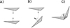 |
Fig. 2. Three cases of geometry for the two facet setup investigated:(a) parallel facets, (b) parallel inclined but nonadjacent facets, and (c) touching facets with a shared edge as a function of angle θ between the planes. |
This parameter can serve as a good criterion for the validity of Eq. (3), and also can be reliably used to optimize subdivision methods in terms of the number of required samples (see Appendix B for example). The number of subdivisions (Ndi = Ndj) are the key parameters for the two M3 methods, and in the following cases we set this number to 256. In the last numerical test we investigate accuracy as a function Ndi, and Ndj to justify this choice. As already noted, the M4 method is taken as a reference value because of its high accuracy, especially for shared-edge and close-by facets (Mazumder & Ravishankar 2012).
In Fig. 3, a parallel facets case is considered. For both panels of the figure, the abscissa shows the Ns metric (Eq. (9)), while the ordinate indicates the view factor F21 (top panel), and relative differences with respect to M4 in the bottom panel. In this scenario, the Ns only varies due to changes in the distance between facets, while areas of the two triangles remain constant. We can immediately see (bottom panel) that the M1 method, as expected, is the least accurate for close distances (small Ns), however, this approach improves in accuracy as we increase the distance between the facets. The M2 method demonstrates improved accuracy in comparison with M1 in this setup. The subdivision techniques are superior in accuracy to both M1 and M2 for the entire range of Ns values. Even at the smallest Ns both M3 approaches reach a sub-percent difference relative to the M4 reference. We should point out that this very high accuracy is contingent on the number of subdivisions, which is taken in this work as Ndi = Ndj = 256. This means that the accuracy of M3 methods can be further improved or degraded by increasing/decreasing Ndi and Ndj, respectively. The improvements in the view factor accuracy come at a computational cost, which are discussed later in this work in connection with a more practical example.
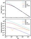 |
Fig. 3. Top: comparison of multiple methods for calculating the view factor F21 for two parallel facets (the case A) in Fig. 2) as a function of Ns (Eq. (9)). Bottom: relative deviation from M4 as a function of Ns for different methods. The standard approach, M1, is accurate to within 1% when Ns is larger than about 100, while the subdivision methods, M3-Linear and M3-R2, are in accurate within 1% for the entire range of Ns. Therefore, these methods are clearly superior to the M1 and M2 methods. |
Figure 4 also has the same two panels as the previous figure. However, these results correspond to the case in which one of the facets is inclined at 45° as illustrated in panel B) in Fig. 2. Naturally, the absolute value of the view factor is reduced compared to the parallel facet example. Here, the relative accuracy between M1 and M2 does not show any difference, and they only reach the 1% mark of accuracy (with regard to M4) for large Ns values of about 500–600. As in the previous case study the two subdivision methods show an accuracy of < 1% for the entire range of Ns values. We can also observe a discontinuity in the relative accuracy curve for the M3-R2 method (also visible in the previous example). This feature, manifesting as a rapid increase in accuracy over a narrow range of Ns values, is purely a numerical artifact of the method. It is related to the mapping of the point via the parallelogram algorithm (see Appendix A). However, its dependence on Ns is not trivial. From these and other tests we see that it depends on the exact shape of the two facets, as well as the angle between them, and the number of sampling points applied. For instance, increasing the Ndi and Ndj over 300 seems to completely eliminate this feature for this test case.
 |
Fig. 4. Top: value of view factor F21 as a function of Ns (Eq. (9)) for a case when one facet is inclined at 45° (the case B) in Fig. 2). The different curves correspond to different methods as labeled. (Bottom) Relative deviation from M4. As in the previous case, even in this case the M3-Linear and M3-R2 methods remain accurate within 1% even for very low Ns values. However, the M3-R2 method does not asymptotically approach the reference value with increasing Ns in this setup. The M2 and M1 agreement shown in this figure is just a coincidence due to facet parameters. |
Figure 5 shows calculations of the view factor F21 as a function of the opening angle between the two facets sharing an edge (panel C) in Fig. 2). The top panel shows the absolute value of F21, while the relative deviation with regards to the M4 method is plotted in the bottom panel. This geometrical setup is challenging for all methods, but in particular for M1 and M2 for small opening angles. In addition, both M1 and M2 methods do not reach better than 10–20% accuracy even for large angles, although the M1 method is not monotonic in its behavior. On the other hand, the two M3 methods show a trend of increasing accuracy for angles larger than 25° until the value of about 170°, where there is a small spike of worsening. The curve for M3-R2 stays more flat with an increasing angle going from about 8% (at 25°) to 5% at 170°. The M3-Linear method starts at ∼10% accuracy reaching a value 1–2% for large opening angles. This result is important especially for modeling cracks, pits, and other concave surface structures. Nevertheless, a physical shape model of a comet or an asteroid is not expected to have two touching facets with an opening angle smaller than perhaps 30–40°, however, there are likely to be many cases of large opening angles (>120°).
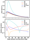 |
Fig. 5. Top: dependence of view factor, F21, in the case of shared-edge facets as a function of the opening angle between these facets (case C) in Fig. 2). As in previous cases, M4 is the reference value. Bottom: relative deviation from M4. The M3-Linear and M3-R2 methods show a reasonable accuracy even for small angles (around 10%). Both methods become more accurate with larger opening angles, although never get to less than 1%. |
In connection with the previous figure (Fig. 5), additional numerical experiments show that when we increase the number of sampling points the M3-R2 method reaches an accuracy of 2–3%. On the other hand, the M3-Linear result improves at slower rate with increasing number of subdivisions. This is demonstrated, in a more general way, in Fig. 6. This is a case of two touching (shared-edge) facets that have 60° opening angle between them. The abscissa shows the different number of subdivisions and sampling points relevant to the two M3 methods, and the ordinate corresponds to the relative deviation in F21 view factor from the reference value, M4. M1 and M2 methods do not depend on subdivision, therefore they keep a constant value. The first thing to note is that the M3-Linear method with a subdivision of zero recovers the M1 view factor value. Then, as the number of subdivisions increases the value approaches the M4 reference, however, this value can reach below about 5% accuracy only for 256 sub-facets. We note that the M3-Linear can increase subdivisions only in steps of 4n for n = 0, 1, …, hence the segmented curve in Fig. 6. The M3-R2 method, as it depends on quasi-random sequence of points, does not behave deterministically for a small number of subdivisions and does not recover the M1 value. In this, as well as other numerical experiments, we observe that a reliable accuracy is reached when using 50–80 sampling points. However, as the number of sampling points is increased, it does approach asymptotically the M4 value and may be marginally better than the M3-Linear approach when number of points exceeds 300–400. The decision of how many sub-facets or samplings to use is the key aspect of both M3 methods from the point of view of accuracy, but also from the point of view of computational speed.
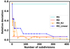 |
Fig. 6. Relative deviation of view factor F21 with respect to M4 for two facets sharing an edge with a 60° opening angle between them, shown as a function of subdivisions of the two triangles. Only the two M3 methods are dependent on the number of subdivision. Both M3-Linear and M3-R2 become more accurate with larger number of subdivisions. We find that around 100 subdivisions the deviation from the reference is about 10% for M3-Linear and about 5% for the M3-R2. However, the M3-R2 is unpredictable for very small number of subdivisions (see text for details). |
Finally, we apply the M1, M4, and both of the M3 methods for view factor calculations for a section of the 67P/CG SHAP7 (Preusker et al. 2017) shape model. The extracted surface shown in Fig. 7 belongs to the northern hemisphere (includes parts of the Seth region) and is made of 1000 facets. It is chosen because it has several interesting topographical features desirable for testing the view factor algorithms. In particular, there is the deep pits/sink hole, for which accurate view factor calculations are important for a long-term evolution models. In Fig. 8 we show results of the accuracy comparisons.
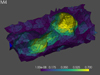 |
Fig. 7. Small subset of SHAP7 shape model of 67P/CG featuring a large pit to be used for performance inter-comparison of the view factor calculation method. The pit can be found in the northern hemisphere of the comet (border of Hapi and Seth region). The color scale corresponds to the total F12 view factor for each facet evaluated with the M4 method, which is used as a reference (true value). In this calculation the effects of the surrounding shape model are not taken into account. However, this should not carry importance for facets inside the pit, which is our main focus in the following comparisons. The bright blue colored facet indicates total view factor below the minimum value of 10−8. |
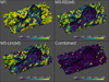 |
Fig. 8. Inter-comparison of the various methods of estimating the view factors for a 1000 facet segment dominated by a large pit. In each of the four panels the color scale represents absolute value percent differences in total view factor of a facet with respect to the M4 method. The limits on the color scale are 0–5%, and facets above this limit are shown in yellow. This includes a couple of facets at the edges of the extracted surface that do not have the visibility of any other facets. The labels in each panel indicate a particular method to which the results belong. The numbers in parentheses indicate the number of sub-facets for the M3 methods, for example, M3-Lin(64) means that M3-Linear with each facet split into 64 sub-facets. A comparison of the “combined” method aimed to optimize speed and accuracy is presented in the bottom right panel, which is detailed in Appendix B. |
The first panel in Fig. 8 shows the percent difference between M1 and M4 calculated as (M1 − M4)/M4. As expected, the M1 method in this example is applied beyond the scope of its assumptions, and the deviation inside the pit are on average around 15%, with couple of smaller facets near the floor and wall of the pit exceeding 50%. In the rugged region surrounding the pit, with many adjacent facets with large opening angles, it also performs poorly. The top right and bottom left panels show the M3-Linear and M3-R2 methods with 64 sub-sampling, respectively. We observe that for facets inside the pit the accuracy at this level of subdivision is acceptable and both methods provide a similar level of accuracy within 0–3%; only few facets have larger deviations. Outside the pits, the view factors absolute values are smaller and mutual facet geometry leads to larger discrepancies of about 20%. Increasing the number of subdivisions to 256 carries a larger computational burden than the more accurate M4 approach, hence it is more suitable to employ the combined method (see Appendix B). This method also offers a good trade-off between accuracy and calculation speed as summarized in Table 1.
4. Conclusions
The goal of this paper is to present quantitative comparisons of several numerical algorithms for calculating view factors. These are routinely required for accurate thermophysical modeling of cometary and asteroid surfaces. In particular, we want to investigate challenging cases of shared-edge facets as a function of the angle between them. Having the accuracy of these calculations under control becomes especially important when modeling energy dissipation inside cracks, pits, and/or fractures. As a benchmark of accuracy we provide the double-line integral method, M4, which does not suffer shortcomings of assumptions inherent in the more typical technique of a facet subdivision. The five methods investigated in this work include the “standard” approaches (M1 and M3-Linear); an analytical solution, M2, which should improve upon M1 for conditions of close distance; and a derivative of the subdivision method based on quasi-random point distribution, M3-R2.
First, we reduced the problem to a two-facet system to clearly demonstrate the performance of each approach as a function of a single parameter, Ns, that combines the distance and areas of the two facets (Eq. (9)). Second, we present a view factor accuracy as a function of opening angle between the triangles with a shared edge, and we also show how the performance depends on number of subdivisions and samples for the two M3 methods.
Finally, we also applied the main algorithms to a subset of 67P/CG surface and discussed the accuracy and computational burden for each method. The main conclusions of this work can be summarized as follows:
-
The view factor calculations transformed into closed loop integral, M4, is the most accurate and it is especially suitable when high accuracy calculations are required for touching or very nearby facets. This is, however, very time consuming, more than two orders of magnitude compared to the most simple solution, M1.
-
The applicability of the simple approach, M1, method, depends on the Ns value and to some degree on the relative orientation of the facets in question. For example, an accuracy of 1% for parallel facets seems to require Ns parameter larger than about 100. However, for facets with smaller opening angles (45° in our case) in our setup these conditions could reach values of 500–600 (see Fig. 4). Nevertheless, if an accuracy of 10–20% is acceptable the M1 method appears to be generally proper for conditions of Ns > 100, provided that facets do not share an edge.
-
We find the accuracy of M2 approach not significantly different from M1 except in cases of few special geometries. We do not see an advantage of using this method for general application to comet or asteroid shape models.
-
The M3-Linear approach, often used in applications to comets or asteroids (e.g., Hu et al. 2017 and references therein), is a viable option for view factor calculations of nearby and/or adjacent facets. However, the number of facet subdivisions used to improve the accuracy plays a crucial role and depends on facet configurations, as shown in Figs. 5 and 6. If the number of sub-facets needs to be increased beyond 64 we found that the combined method presented in Appendix B offers a better choice in terms of accuracy and computational speed.
-
5.
The M3-R2 method also turns out to perform well, being able to deal with nearby or shared-edge facets. For the same number of sampling points it is very close in accuracy to the M3-Linear approach and even may outperform it for selected cases of geometry. This method has the advantage that the number of sampling points can be optimized easily, it is simpler to implement, and the computational burden is about 20% less than the M3-Linear. However, this approach relies on a quasi-random sequence of points distributed over a facet, hence, it cannot be used for number of sampling points smaller than about 60 (an empirical finding). In addition, this method does not behave predictably for low number of sampling points.
-
6.
In larger scale applications where the view factor accuracy is a crucial aspect we suggest combining the methods M1, (M3-Linear or, M3-R2) with M4 to strike a good balance between accuracy and speed. We present an algorithm in appendix B, which we used in this work to reach an average accuracy inside the pit better than 2% (Fig. 8). The algorithm is robust in that it relies on the Ns metric to decide which method to apply and how many subdivisions to use. However, there are still several tuning parameters (the constants used in the algorithm) that allow a user the freedom to adjust to trade between accuracy and speed, depending on the nature of the problem at hand.
As a final remark, we acknowledge that our numerical implementation of the discussed algorithms is not optimized for calculation speed. The absolute, perhaps even the relative times, might be improved with a more rigorous approach (taking advantage of implementation in compiled programming language, hardware acceleration, and/or better parallelization). This work made use of the open source software PyVista (Sullivan & Kaszynski 2019) to produce Fig. 8 and for efficient M3-Linear facet subdivision implementation.
Acknowledgments
We would like to thank Yuri Skorov and H. U. Keller for their time, the many discussions around this topic and general encouragement to complete this work. LR acknowledges support from the project DFG-392267849. YZ was supported from the National Natural Science Foundation of China (Grant No: 11761131008, 11673072), the Strategic Priority Research Program on Space Science(CAS) (Grant No. XDA15017600) and the Foundation of Minor Planets of Purple Mountain Observatory.
References
- Abaqus 2020, Abaqus View Factor Calculations [Google Scholar]
- Ambirajan, A., & Venkateshan, S. 1993, Int. J. Heat Mass Trans., 36, 2203 [CrossRef] [Google Scholar]
- Baranoski, G. V., Rokne, J. G., & Xu, G. 2001, J. Quant. Spectr. Rad. Trans., 69, 447 [CrossRef] [Google Scholar]
- Colwell, J. E., Jakosky, B. M., Sandor, B. J., & Stern, S. 1990, Icarus, 85, 205 [NASA ADS] [CrossRef] [Google Scholar]
- Davidsson, B. J., & Rickman, H. 2014, Icarus, 243, 58 [NASA ADS] [CrossRef] [Google Scholar]
- Delbo, M., Mueller, M., Emery, J. P., Rozitis, B., & Capria, M. T. 2015, Asteroid Thermophysical Modeling (Arizona: University of Arizona Press Tucson) [Google Scholar]
- Francisco, S., Raimundo, A., Gaspar, A., Oliveira, A. V., & Quintela, D. 2014, J. Build. Perform. Simul., 7, 203 [CrossRef] [Google Scholar]
- Gutiérrez, P. J., Ortiz, J. L., Rodrigo, R., & López-Moreno, J. J. 2001, A&A, 374, 326 [NASA ADS] [CrossRef] [EDP Sciences] [Google Scholar]
- Hamm, M., Grott, M., Kührt, E., Pelivan, I., & Knollenberg, J. 2018, Planet. Space Sci., 159, 1 [CrossRef] [Google Scholar]
- Howell, J. R., Menguc, M. P., & Siegel, R. 2010, Thermal Radiation Heat Transfer (CRC Press) [CrossRef] [Google Scholar]
- Hu, X., Shi, X., Sierks, H., et al. 2017, MNRAS, 469, S295 [CrossRef] [Google Scholar]
- Ivanova, A. V., & Shulman, L. M. 2006, Adv. Space Res., 38, 1932 [NASA ADS] [CrossRef] [Google Scholar]
- Kramer, S., Gritzki, R., Perschk, A., Rasler, M., & Felsmann, C. 2015, Int. J. Therm. Sci., 96, 345 [CrossRef] [Google Scholar]
- Lagerros, J. S. V. 1997, A&A, 325, 1226 [NASA ADS] [Google Scholar]
- Maltby, J. D., & Burns, P. J. 1991, Numer. Heat Trans. Part B Fundam., 19, 191 [CrossRef] [Google Scholar]
- Mazumder, S., & Ravishankar, M. 2012, Int. J. Heat Mass Trans., 55, 7330 [CrossRef] [Google Scholar]
- Mirhosseini, M., & Saboonchi, A. 2011, Int. Commun. Heat Mass Trans., 38, 821 [CrossRef] [Google Scholar]
- Modest, M. 1978, Numer. Heat Trans. Part B Fundam., 1, 403 [CrossRef] [Google Scholar]
- Modest, M. 2003, Radiative Heat Transfer, II edn. (NewYork, Oxford, Tokyo): (Academic Press) [Google Scholar]
- Modest, M. F. 2013, Radiative Heat Transfer (Third Edition) (Boston: Academic Press), 129 [CrossRef] [Google Scholar]
- Narayanaswamy, A. 2015, Int. J. Heat Mass Trans., 91, 841 [CrossRef] [Google Scholar]
- Ozisik, M. N. 1985, Heat Transfer: a Basic Approach (New York: McGraw-Hill), 1 [Google Scholar]
- Pelivan, I. 2018, MNRAS, 478, 386 [CrossRef] [Google Scholar]
- Preusker, F., Scholten, F., Matz, K.-D., et al. 2017, A&A, 607, L1 [NASA ADS] [CrossRef] [EDP Sciences] [Google Scholar]
- Roberts, M. 2018, The Unreasonable Effectiveness of Quasirandom Sequences [Google Scholar]
- Rozitis, B., & Green, S. F. 2011, MNRAS, 415, 2042 [NASA ADS] [CrossRef] [Google Scholar]
- Shi, X., Hu, X., Sierks, H., et al. 2016, A&A, 586, A7 [NASA ADS] [CrossRef] [EDP Sciences] [Google Scholar]
- Siegel, R., & Howell, J. 2002, Thermal Radiation Heat Transfer (Taylor & Francis Group) [Google Scholar]
- Sparrow, E. M. 1963, J. Heat Transfer, 81 [Google Scholar]
- Sullivan, C. B., & Kaszynski, A. 2019, J. Open Source Soft., 4, 1450 [CrossRef] [Google Scholar]
- Vujičić, M., Lavery, N., & Brown, S. 2006, Commun. Numer. Methods Eng., 22, 197 [Google Scholar]
- Warren, J., & Weimer, H. 2001, Subdivision Methods for Geometric Design: A Constructive Approach (Morgan Kaufmann Publishers Inc.) [Google Scholar]
- Yarbrough, D. W., & Lee, C.-L. 1986, Integral Methods in Science and Engineering (Harper and Rowe/Hemisphere), 563 [Google Scholar]
- Zhao, Y., Rezac, L., Skorov, Y., & Li, J.-Y. 2020, MNRAS, 492, 5152 [CrossRef] [Google Scholar]
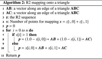
Appendix A: M3-R2: Distribution of quasi-random points over triangle
An algorithm for calculating the low discrepancy quasi-random sequence, and mapping them over an arbitrary shaped triangle in described in this appendix. We provide this algorithm for convenience since, as pointed out, the original work is only available in online form (Roberts 2018).2
In the first step, we generate the two-dimensional R2 quasi-random sequence with n points following the given algorithm:
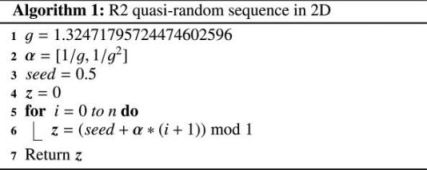
What remains to be pointed out is that the R2 sequence is sensitive to the seed value and should remain as set in this appendix.
We follow recommended parallelogram method to map the R2 sequence onto a triangle. This is a simple yet effective way in preserving low discrepancy point distribution in a triangle without aliasing.
An example of a quasi-random, low discrepancy distribution of points via the M3-R2 method is contrasted with “random” point distribution in Fig. A.1. The random distribution of points seems inefficient in evenly covering the area of a triangle and would require a large number of sampling points for required accuracy. Within an acceptable error (see results, section 4) the M3-R2 method is more evenly distributed (low discrepancy) and allows for a fast area subdivision of a facet.
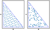 |
Fig. A.1. Left: one hundred sampling points distributed on a triangle via the R2 method, and (right) 100 sample points from a uniform random number generator mapped onto the same triangle. The low discrepancy (the largest possible distance among the points) of R2 method is well demonstrated, producing a homogeneous coverage that allows for a quick, implicit area subdivision. |
Appendix B: Combined algorithm for view factor calculations
We present an algorithm for view factor calculation combining the M1, M3-Linear (M3-R2 could be substituted ), and M4 method. The algorithm relies on the Ns metric (Eq. (9)) and the dot product between the two normal vectors of facets in question to select which method is applicable. The Ns also determines the number of sub-samplings (or sub-facets) when either of the M3 methods is used. We would like to point out that for the linear method the subdivision can be scaled only as 4n, and in this algorithm we do not allow n smaller than two, effectively yielding Nd of either 8 or 64. Also, we opted out for the M3-Linear instead of the slightly faster M3-R2 method due overall smaller scatter in accuracy as shown in Fig. C.1.
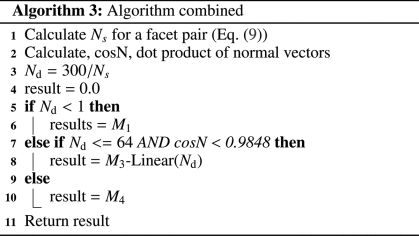
Appendix C: Inter-comparisons of methods for view factor computations
Figure C.1 summarizes the accuracy and precision of the presented algorithms for view factor calculations. In this comparison we selected facets with Fij > 0.01, which includes all the facets inside the large and small pits (Fig. 7). The circle marker represents the mean percent difference with respect to the M4 reference and error bars correspond to the 1 sigma standard deviation. Although on average the method M1 shows acceptable accuracy (∼2.5%) the size of the error bars indicates rather large deviations among the facets; this is also seen in Fig. 8, where many facets show significantly larger deviation. Increasing subdivision number of M3-Linear method from 64 to 256 marginally improves the overall accuracy and reduces the deviations among individual facets. A similar conclusion is reached for the R2 method, however, it has noticeably larger deviations compared to the M3-Linear for the same number of subdivisions. The combined method, as given in the algorithm in Appendix B, provides excellent agreement and very small deviations (which are about the size of the marker). This plots highlights the advantage of using the combined method, which balances speed and accuracy.
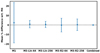 |
Fig. C.1. Summary of mean accuracy and overall precision of the main methods of view factor calculations studied in this paper (see text for description). |
All Tables
All Figures
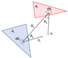 |
Fig. 1. Geometry and illustration of parameters used in Eq. (1) to calculate the view factor Fij. |
| In the text | |
|
Fig. 2. Three cases of geometry for the two facet setup investigated:(a) parallel facets, (b) parallel inclined but nonadjacent facets, and (c) touching facets with a shared edge as a function of angle θ between the planes. |
| In the text | |
|
Fig. 3. Top: comparison of multiple methods for calculating the view factor F21 for two parallel facets (the case A) in Fig. 2) as a function of Ns (Eq. (9)). Bottom: relative deviation from M4 as a function of Ns for different methods. The standard approach, M1, is accurate to within 1% when Ns is larger than about 100, while the subdivision methods, M3-Linear and M3-R2, are in accurate within 1% for the entire range of Ns. Therefore, these methods are clearly superior to the M1 and M2 methods. |
| In the text | |
|
Fig. 4. Top: value of view factor F21 as a function of Ns (Eq. (9)) for a case when one facet is inclined at 45° (the case B) in Fig. 2). The different curves correspond to different methods as labeled. (Bottom) Relative deviation from M4. As in the previous case, even in this case the M3-Linear and M3-R2 methods remain accurate within 1% even for very low Ns values. However, the M3-R2 method does not asymptotically approach the reference value with increasing Ns in this setup. The M2 and M1 agreement shown in this figure is just a coincidence due to facet parameters. |
| In the text | |
|
Fig. 5. Top: dependence of view factor, F21, in the case of shared-edge facets as a function of the opening angle between these facets (case C) in Fig. 2). As in previous cases, M4 is the reference value. Bottom: relative deviation from M4. The M3-Linear and M3-R2 methods show a reasonable accuracy even for small angles (around 10%). Both methods become more accurate with larger opening angles, although never get to less than 1%. |
| In the text | |
|
Fig. 6. Relative deviation of view factor F21 with respect to M4 for two facets sharing an edge with a 60° opening angle between them, shown as a function of subdivisions of the two triangles. Only the two M3 methods are dependent on the number of subdivision. Both M3-Linear and M3-R2 become more accurate with larger number of subdivisions. We find that around 100 subdivisions the deviation from the reference is about 10% for M3-Linear and about 5% for the M3-R2. However, the M3-R2 is unpredictable for very small number of subdivisions (see text for details). |
| In the text | |
|
Fig. 7. Small subset of SHAP7 shape model of 67P/CG featuring a large pit to be used for performance inter-comparison of the view factor calculation method. The pit can be found in the northern hemisphere of the comet (border of Hapi and Seth region). The color scale corresponds to the total F12 view factor for each facet evaluated with the M4 method, which is used as a reference (true value). In this calculation the effects of the surrounding shape model are not taken into account. However, this should not carry importance for facets inside the pit, which is our main focus in the following comparisons. The bright blue colored facet indicates total view factor below the minimum value of 10−8. |
| In the text | |
|
Fig. 8. Inter-comparison of the various methods of estimating the view factors for a 1000 facet segment dominated by a large pit. In each of the four panels the color scale represents absolute value percent differences in total view factor of a facet with respect to the M4 method. The limits on the color scale are 0–5%, and facets above this limit are shown in yellow. This includes a couple of facets at the edges of the extracted surface that do not have the visibility of any other facets. The labels in each panel indicate a particular method to which the results belong. The numbers in parentheses indicate the number of sub-facets for the M3 methods, for example, M3-Lin(64) means that M3-Linear with each facet split into 64 sub-facets. A comparison of the “combined” method aimed to optimize speed and accuracy is presented in the bottom right panel, which is detailed in Appendix B. |
| In the text | |
|
Fig. A.1. Left: one hundred sampling points distributed on a triangle via the R2 method, and (right) 100 sample points from a uniform random number generator mapped onto the same triangle. The low discrepancy (the largest possible distance among the points) of R2 method is well demonstrated, producing a homogeneous coverage that allows for a quick, implicit area subdivision. |
| In the text | |
|
Fig. C.1. Summary of mean accuracy and overall precision of the main methods of view factor calculations studied in this paper (see text for description). |
| In the text | |
Current usage metrics show cumulative count of Article Views (full-text article views including HTML views, PDF and ePub downloads, according to the available data) and Abstracts Views on Vision4Press platform.
Data correspond to usage on the plateform after 2015. The current usage metrics is available 48-96 hours after online publication and is updated daily on week days.
Initial download of the metrics may take a while.