Search and analysis of giant radio galaxies with associated nuclei (SAGAN)

P. Dabhade; M. Mahato; J. Bagchi; D. J. Saikia; F. Combes; S. Sankhyayan; H. J. A. Röttgering; L. C. Ho; M. Gaikwad; S. Raychaudhury; B. Vaidya; B. Guiderdoni

doi:10.1051/0004-6361/202038344

Home

All issues

Volume 642 (October 2020)

A&A, 642 (2020) A153

Full HTML

Free Access

Issue		A&A Volume 642, October 2020


Article Number		A153
Number of page(s)		31
Section		Extragalactic astronomy
DOI		https://doi.org/10.1051/0004-6361/202038344
Published online		13 October 2020

A&A 642, A153 (2020)

I. New sample and multi-wavelength studies^⋆

P. Dabhade¹^,2, M. Mahato², J. Bagchi², D. J. Saikia², F. Combes³^,4, S. Sankhyayan²^,5^,6, H. J. A. Röttgering¹, L. C. Ho⁷^,8, M. Gaikwad⁹, S. Raychaudhury²^,10, B. Vaidya¹¹ and B. Guiderdoni¹²

¹ Leiden Observatory, Leiden University, PO Box 9513, 2300 RA Leiden, The Netherlands
e-mail: pratik@strw.leidenuniv.nl
² Inter-University Centre for Astronomy and Astrophysics (IUCAA), Pune 411007, India
³ Sorbonne Université, Observatoire de Paris, Université PSL, CNRS, LERMA, 75014 Paris, France
⁴ Collège de France, 11 Place Marcelin Berthelot, 75231 Paris, France
⁵ Indian Institute of Science Education and Research (IISER), Dr. Homi Bhabha Road, Pashan, Pune 411008, India
⁶ National Centre for Radio Astrophysics, TIFR, Post Bag 3, Ganeshkhind, Pune 411007, India
⁷ Kavli Institute for Astronomy and Astrophysics, Peking University, Beijing 100871, PR China
⁸ Department of Astronomy, School of Physics, Peking University, Beijing 100871, PR China
⁹ Max-Planck-Institut für Radioastronomie, Auf dem Hugel 69, 53121 Bonn, Germany
¹⁰ Department of Physics, Presidency University, 86/1 College Street, Kolkata 700073, India
¹¹ Discipline of Astronomy, Astrophysics and Space Engineering, Indian Institute of Technology Indore, Indore 453552, India
¹² Univ. Lyon, ENS de Lyon, CNRS, Centre de Recherche Astrophysique de Lyon, 69230 Saint-Genis-Laval, France

Received: 3 May 2020
Accepted: 5 August 2020

Abstract

We present the first results of a project called SAGAN, which is dedicated solely to the studies of relatively rare megaparsec-scale radio galaxies in the Universe, called giant radio galaxies (GRGs). We have identified 162 new GRGs primarily from the NRAO VLA Sky Survey with sizes ranging from ∼0.71 Mpc to ∼2.82 Mpc in the redshift range of ∼0.03−0.95, of which 23 are hosted by quasars (giant radio quasars). As part of the project SAGAN, we have created a database of all known GRGs, the GRG catalogue, from the literature (including our new sample); it includes 820 sources. For the first time, we present the multi-wavelength properties of the largest sample of GRGs. This provides new insights into their nature. Our results establish that the distributions of the radio spectral index and the black hole mass of GRGs do not differ from the corresponding distributions of normal-sized radio galaxies (RGs). However, GRGs have a lower Eddington ratio than RGs. Using the mid-infrared data, we classified GRGs in terms of their accretion mode: either a high-power radiatively efficient high-excitation state, or a radiatively inefficient low-excitation state. This enabled us to compare key physical properties of their active galactic nuclei, such as the black hole mass, spin, Eddington ratio, jet kinetic power, total radio power, magnetic field, and size. We find that GRGs in high-excitation state statistically have larger sizes, stronger radio power, jet kinetic power, and higher Eddington ratio than those in low-excitation state. Our analysis reveals a strong correlation between the black hole Eddington ratio and the scaled jet kinetic power, which suggests a disc-jet coupling. Our environmental study reveals that ∼10% of all GRGs may reside at the centres of galaxy clusters, in a denser galactic environment, while the majority appears to reside in a sparse environment. The probability of finding the brightest cluster galaxy as a GRG is quite low and even lower for high-mass clusters. We present new results for GRGs that range from black hole mass to large-scale environment properties. We discuss their formation and growth scenarios, highlighting the key physical factors that cause them to reach their gigantic size.

Key words: galaxies: active / galaxies: clusters: general / galaxies: jets / radio continuum: galaxies / quasars: general

^⋆

Tables A1–A4 are only available at the CDS via anonymous ftp to cdsarc.u-strasbg.fr (130.79.128.5) or via http://cdsarc.u-strasbg.fr/viz-bin/cat/J/A+A/642/A153

© ESO 2020

1. Introduction

In the 1950s, it was revealed that some galaxies dominantly emit at radio wavelengths (Jennison & Das Gupta 1953; Baade & Minkowski 1954) through synchrotron radiation (Shklovskii 1955; Burbidge 1956). These galaxies later came to be known as radio galaxies (RGs), whose radio emission often extends well beyond the physical extent of the galaxies as seen at optical wavelengths. Thereafter, it was realised by theoretical efforts (Salpeter 1964; Lynden-Bell 1969; Bardeen 1970) that a supermassive black hole (10⁶−10¹⁰ M_⊙) residing at the centre of host galaxy must be responsible for powering (Rees 1971) the radio galaxy through twin collimated and relativistic jets (Blandford & Rees 1974; Scheuer 1974). The creation of the relativistic radio jets is not completely understood and is currently under investigation. Astrophysical models (Blandford & Znajek 1977; hereafter B − Z, Blandford & Payne 1982; Meier et al. 2001) show that they are created by mass-accreting black holes with a certain geometry of the magnetic field that threads the accretion disc.

The B − Z model describes the process that is thought to be responsible for powering jets in galactic microquasars and gamma-ray bursts in addition to radio galaxies and quasars. It has been established in many studies over the years that supermassive black holes (SMBHs) reside at the centres of almost all massive galaxies (Soltan 1982; Rees 1984; Begelman et al. 1984; Magorrian et al. 1998; Kormendy & Ho 2013), and their active phase is triggered only under certain circumstances. These active forms of SMBHs are known as the active galactic nuclei (AGNs), whose signatures can be observed at almost all wavelengths, ranging from radio to gamma-rays.

Those AGNs that predominantly emit at radio wavelengths are called radio-loud AGNs (RLAGNs). A smaller fraction and more powerful class of AGNs are quasars, which are among the most energetic and brightest objects known in the Universe. When quasar AGNs emit radiation at radio wavelengths, they are called radio-loud quasars (RQs). In high-luminosity RGs or RQs, the jets tend to terminate in high-brightness regions, called hotspots, at the outer edges of the radio lobes, which are filled with relativistic non-thermal plasma. This class of RGs is the Fanaroff-Riley II (FR-II) class (Fanaroff & Riley 1974). FR-IIs are edge-brightened RGs, and the Fanaroff-Riley I (FR-I) class RGs are less powerful than FR-II. The FR-I structure is mainly edge-darkened and lobe brightness peaks within the inner half of their extent; they have no hotspot. The largest angular size is usually measured between the peaks in the hotspots for FR-II sources and the outermost contours at the 3σ level for FR-I sources. The projected linear size of RGs or RQs extends from less than a few kilo parsecs (pc) to several megaparsecs (Mpc).

In the past six decades, thousands of RGs have been found and catalogued, but only a few hundred RGs have been discovered so far to exhibit Mpc-scale sizes. Since their discovery in the 1970s by Willis et al. (1974), this relatively rare sub-class of RGs has been referred to by several names, such as “giant radio sources” (GRSs), “large radio galaxies” (LRGs), and “giant radio galaxies” (GRGs). In order to avoid confusion and to maintain uniformity, we refer to this giant sub-class of RGs as “giant radio galaxies” (GRGs), as previously adopted in several works (Schoenmakers et al. 2001; Dabhade et al. 2017, 2020; Ursini et al. 2018).

Since the discovery of GRGs in the 1970s to early-2000s, the Hubble constant (H₀) that is used to derive the physical properties of the GRGs had a range of values between 50 and 100 km s⁻¹ Mpc⁻¹ based on available measurements at that time. This led to over- or under-estimating the sizes of these sources and eventually to inaccurate statistics of their population. With the advent of precision cosmology derived from the cosmic microwave background radiation observed with the Wilkinson Microwave Anisotropy Probe (WMAP; Hinshaw et al. 2013) and Planck mission (Planck Collaboration XIII 2016), the value of H₀ was set to ∼68 km s⁻¹ Mpc⁻¹. The first GRGs discovered by Willis et al. (1974) were 3C236 and DA240, both of which are more than 2 Mpc in size, and hence they did not set a lower size limit for RGs to be classified as GRGs. Later studies (Ishwara-Chandra & Saikia 2000; Schoenmakers et al. 2001) adopted a lower limit of 1 Mpc, assuming H₀ to 50 km s⁻¹ Mpc⁻¹. Recent studies (Dabhade et al. 2017, 2020; Kuźmicz et al. 2018; Ursini et al. 2018) have adopted 700 kpc as the lower size limit of GRGs with the updated H₀ value obtained from observations.

In the past six decades, owing to radio surveys such as the third Cambridge radio survey (3CR; Bennett 1962; Laing et al. 1983), the Bologna Survey (B2; Colla et al. 1970), the Faint Images of the Radio Sky at Twenty-Centimeters survey (FIRST; Becker et al. 1995), the NRAO VLA Sky Survey (NVSS; Condon et al. 1998), the Westerbork Northern Sky Survey (WENSS; Rengelink et al. 1997), the Sydney University Molonglo Sky Survey (SUMSS; Bock et al. 1999), the TIFR GMRT Sky Survey (TGSS; Intema et al. 2017), and the LOFAR Two-metre Sky Survey (LoTSS; Shimwell et al. 2019), millions of RGs have been found, and a considerable fraction has been studied in detail. However, only a few hundred of these RGs have been identified as giants or GRGs. The relatively small number of GRGs might partly be due to difficulties in identifying them. Possible factors include the detection of low surface brightness components, ensuring that two radio components are indeed related, and finding confirmed optical counterparts. However, when we take a complete radio sample such as the 3CRR sample (Laing et al. 1983), the median size¹ of the RGs or RQs is ∼350 kpc, and only ∼7% of the sample are GRGs.

Over a course of about 45 years, about 40 research papers (Willis et al. 1974; Bridle et al. 1976; Waggett et al. 1977; Laing et al. 1983; Kronberg et al. 1986; de Bruyn 1989; Jones 1989; Ekers et al. 1989; Lacy et al. 1993; Law-Green et al. 1995; Cotter et al. 1996; McCarthy et al. 1996; Subrahmanyan et al. 1996; Ishwara-Chandra & Saikia 1999; Lara et al. 2001; Machalski et al. 2001, 2007, 2008; Kozieł-Wierzbowska & Stasińska 2011; Schoenmakers et al. 2001; Sadler et al. 2002; Letawe et al. 2004; Saripalli et al. 2005; Saikia et al. 2006; Huynh et al. 2007; Hota et al. 2011; Solovyov & Verkhodanov 2014; Molina et al. 2014; Bagchi et al. 2014; Amirkhanyan et al. 2015; Tamhane et al. 2015; Amirkhanyan 2016; Dabhade et al. 2017, 2020; Clarke et al. 2017; Kapińska et al. 2017; Prescott et al. 2018; Sebastian et al. 2018; Kuźmicz et al. 2018; Kozieł-Wierzbowska et al. 2020) have reported about 662 GRGs spread throughout the sky. This estimate is based on a database of GRGs that is compiled by us, for which we adopted 700 kpc as the lower limit of GRG size. We used concordant cosmological parameters from Planck (H₀ = 67.8 km s⁻¹ Mpc⁻¹, Ω_m = 0.308, Ω_Λ = 0.692; Planck Collaboration XIII 2016).

Some of the open questions related to GRGs are the processes through which they grow to Mpc-scale sizes, how rare they are with respected normal radio galaxies, do they host most powerful SMBHs, nature of their accretion states, and how fast their SMBHs are spinning. Owing to their enormous sizes, it essential to investigate whether they grow only in sparser environments, and their contribution to large-scale processes.

Giant radio galaxies are the largest single objects in the Universe. They pose interesting questions related to the formation and evolution of such large structures through relativistic jets that originate in SMBHs. These large RGs must be supplied with energy either continuously or quasi-continuously over timescales of at least 10⁷−10⁸ years when we consider that the hotspots (terminal shocks of the jet) move with sub-relativistic speeds (Best et al. 1995; Scheuer 1995; Arshakian & Longair 2000) of ∼0.1c, although highly asymmetric sources such as the apparently one-sided GRGs may require higher velocities (Saikia et al. 1990). It has been suggested that their evolution to such large sizes is due to their occurrence in low-density environments (Mack et al. 1998; Pirya et al. 2012; Malarecki et al. 2015; Saripalli & Malarecki 2015). Pirya et al. (2012) found that GRGs are usually located in low galaxy density environments by counting galaxies in the vicinity of GRGs. However, the structural asymmetries in their sample of giants, in which the nearer component is often brighter, suggest asymmetries in the intergalactic medium that are not apparent from examining the galaxy distribution. Only in the case of 3C326 did they find the closer brighter arm to be possibly interacting with a group of galaxies that is part of a larger filamentary structure. Machalski et al. (2008) reported the discovery of the largest GRG J1420−0545 and suggested that the source is located in a very low-density environment and has a high expansion speed along the jet axis. However, a few studies, such as Komberg & Pashchenko (2009) and Dabhade et al. (2017, 2020), have shown dozens of GRGs residing in dense cluster environments. A few other studies (Subrahmanyan et al. 1996; Saripalli et al. 2005; Bruni et al. 2019, 2020) have also suggested that GRGs may attain their gigantic size due to the restarted AGN activity. Different explanations may be applicable to different subsets of GRGs, which detailed studies of large samples and comparisons with theoretical models and simulations will help clarify (e.g. Hardcastle 2018a, and references therein).

It has also been suggested that GRGs contain exceptionally powerful central engines that are powered by massive black holes, which are responsible for their gigantic sizes (Gopal-Krishna et al. 1989). Based on the current understanding, the environment alone therefore cannot be the only determining factor for the giant size of GRGs, but a combination of AGN power (including jet power and accretion states), environmental factors, and the longevity of AGN activity (duty cycle) might be playing an equally important role.

Moreover, multi-wavelength studies of only a small fraction of GRGs have been carried out so far to specifically address the important questions related to their unusual nature. This has restricted a comprehensive statistical analysis of the properties of GRGs to understand their true nature.

In order to address these questions in a systematic study of a large number of GRGs, we have initiated a project that is completely dedicated to the study of GRGs, We describe this in the following parts of this paper along with our first results. For the first time, we have been able to obtain a good understanding of the GRG astrophysics here, spanning an enormous range (∼10¹¹) of physical scales from ∼10⁻⁵ pc in the jet launch zone that lies in the vicinity of the black hole to ∼1 Mpc, where the jet termination point is located.

The paper is organised as follows: in Sect. 2 we present an overview and the goals of project SAGAN. In Sect. 2.1 we describe the search criteria and method for identifying the new GRG sample from the NVSS survey, followed by a discussion of the newly created GRG database in Sect. 2.2. In Sect. 3 we describe the analysis methods we employed on multi-wavelength data of GRGs to estimate their various properties. Next, we present the results of the analysis along with a discussion and their implications in Sect. 4, which is further sub-divided into several subsections, each dedicated to a property of GRGs. We conclude our study of GRGs in project SAGAN and outline its future prospects in Sect. 7. Lastly, in appendix we present three main tables consisting of the properties of our new GRG sample, and in Appendix C we show the multi-frequency radio maps of the GRGs in our new sample.

Throughout this paper, the flat ΛCDM cosmological model is adopted based on the Planck results (H₀ = 67.8 km s⁻¹ Mpc⁻¹, Ω_m = 0.308, and Ω_Λ = 0.692 Planck Collaboration XIII 2016). All the images are presented in a J2000 coordinate system. We use the convention S_ν ∝ ν^−α, where S_ν is the flux density at frequency ν, and α is the spectral index.

2. Project SAGAN

To understand the physics of these extreme cosmic radio sources much better, and specifically, to address the key questions that remain, we have initiated a project called SAGAN² (Search and analysis of GRGs with associated nuclei), whose pilot study results were presented in the previous paper (Dabhade et al. 2017). Some of the main goals for this project are listed below.

1. We aim to create a complete and uniform database of GRGs from the literature, which spans five decades starting from 1970s, using a single cosmological model with H₀ = 67.8 km s⁻¹ Mpc⁻¹, Ω_m = 0.308, and Ω_Λ = 0.692 (flat ΛCDM).

2. We search for more GRGs from existing radio and optical or infrared survey data.

3. Using the newly created large database of GRGs, we carry out multi-wavelength studies of the host AGNs of the GRGs. We intend to focus on some key physical properties such as the accretion rate (̇m) of the black hole, excitation type, black hole mass (M_BH), Eddington ratio, spin, host galaxy star formation rate (SFR), and high-energy gamma-ray emission from jets.

4. We explore effects of the environment on the morphology and growth of the GRGs.

5. We use magneto-hydrodynamical (MHD) simulations to investigate the jet physics and the conditions required for the collimation and stability of relativistic jets, propagating to megaparsec or larger physical distances from the host AGN.

Broadly, the goal is to understand birth, growth, and evolution of GRGs and their possible contribution to other processes in the Universe.

In this first paper, we present the results of our search for GRGs from the NVSS along with GRGs from other published works and investigate their multi-wavelength properties (in radio, optical, and mid-infrared bands). We not only report a larger sample of 162 hitherto unidentified GRGs, but also shed light for the first time on their AGN and host galaxy physical properties.

2.1. New sample of GRGs from NVSS

The NVSS provides radio maps (δ > −40°, 82% of the sky) at 1400 MHz with a modest resolution of 45″ and has root mean square (rms) brightness fluctuations of ∼0.45 mJy beam⁻¹. The NVSS was released more than 20 years ago, and still it continues to be a source of many interesting discoveries (e.g. for GRGs; Solovyov & Verkhodanov 2011; Amirkhanyan 2016; Proctor 2016; Dabhade et al. 2017).

Proctor (2016) produced a catalogue of 1616 possible giant radio sources (GRSs) from automated pattern-recognition techniques using NVSS data. This catalogue of 1616 sources represents the radio objects that are candidates for GRGs with projected angular size ≥4′. Therefore this catalogue serves as a useful database for finding new GRGs.

Following-up on our pilot study, Dabhade et al. (2017), we further carried out our independent manual visual search for GRGs from the NVSS, and the results of the search were combined with the fraction of GRGs we confirmed from the Proctor (2016) sample. In order to confirm potential GRGs from Proctor’s sample, we used the following radio surveys, which complement each other, to understand the radio morphology of the sources:

– NVSS: It has a high sensitivity for large-scale diffuse emission and is one of the best all-sky radio surveys to date.

– FIRST: This survey is at 1400 MHz with a resolution of ∼5″ and 0.15 mJy beam⁻¹ rms. Its high-resolution maps provide vital information about the radio cores and hotspots of the sources.

– TGSS: This is a low-frequency radio survey at 150 MHz with a resolution of ∼25″ and an rms of ∼3.5 mJy beam⁻¹, covering the entire NVSS footprint. It is sensitive to diffuse low radio frequency emission and particularly good at detecting sources with very steep spectra.

– VLASS³: The Very Large Array Sky Survey (Lacy et al. 2020). This is the most recent all-sky radio survey at 3000 MHz with a resolution of ∼2.5″ and rms of ∼100 μJy and covers the same footprint as the NVSS. This survey is deeper, has a better resolution, and covers a greater sky area than the FIRST. It is very useful for identifying compact structures such as the radio cores of the sources.

After the overall morphology of the sources was determined using the available radio surveys, optical and mid-IR data from the Sloan Digital Sky Survey (SDSS; York et al. 2000; Abolfathi et al. 2018), the Panoramic Survey Telescope and Rapid Response System (Pan-STARRS; Kaiser et al. 2002, 2010; Chambers et al. 2016), and the Wide-field Infrared Survey Explorer (WISE; Wright et al. 2010), respectively, were used to identify the host galaxies of the candidate GRGs.

The following steps and criteria were used to create the final sample of confirmed GRGs from the Proctor (2016) GRS catalogue:

1. Optical/mid-IR and radio maps were overlaid to identify the host galaxy/AGN that coincides with the radio core. Sources that did not have a radio core-host galaxy association were rejected.

2. We selected only those sources via thorough manual inspection whose various components (core, jets, or lobes) were sufficiently well resolved, with no ambiguity in their radio morphology.

3. All the sources selected by the above steps were checked for redshift (z) information of the host galaxy (photometric or spectroscopic) from publicly available optical surveys and databases.

4. The angular sizes of the sources were computed using NVSS radio maps for uniformity, and to ensure that there is no flux or structure loss, which the other higher resolution radio surveys (FIRST, TGSS, and VLASS) are prone to. We measured the largest angular separation of the two components (lobes, hotspots, tails, and jets) of the sources after considering only the parts of the sources that are seen above 3σ. In this way, the angular sizes of all the sources were revised, and the angular extent of some sources was < 4′, which is the lower limit of the Proctor (2016) sample.

5. Lastly, we made use of redshift and angular size information to compute the projected linear size of the sources, and only those greater than 700 kpc were considered for our GRG sample (SAGAN GRG sample, or SGS henceforth).

These steps resulted in identifying 151 new GRGs from the Proctor (2016) sample. We also classified the remaining sources into different categories, which can be useful to the scientific community for future work. The classification was made based on the availability of radio and optical data, which are given in Table 1. Many sources from our independent manual search were in common with Proctor (2016) sample, and a total of 11 GRGs were found to be unique (not in the Proctor 2016 sample). After combining the two, we therefore report our final sample (SGS) of 162 GRGs as seen in Table A.1. The sample is discussed in more detail in Sect. 4.

Table 1.

Short summary of the classification of sources from Proctor (2016).

The basic information of the SGS, that is, right ascension (RA) and declination (Dec) of host galaxies in optical, AGN type (galaxy or quasar), redshift, angular size (arcminute), physical size or projected linear size (Mpc), flux density (mJy), and radio powers (W Hz⁻¹) at 1400 MHz and 150 MHz, and spectral index with error estimates are presented in the Table A.1. About 37.7% of the SGS have photometric redshifts, and the remainder has spectroscopic redshift information. When we consider the lower end of the uncertainties of the photometric redshifts obtained from the SDSS, only three sources in our SGS, SAGANJ010052.6+061641.01, SAGANJ075931.84+082534.59, and SAGANJ125204.82−222645.70, are below the cutoff of 0.7 Mpc. The lower limits of their projected linear sizes are 0.68, 0.67, and 0.69 Mpc, respectively.

2.2. The GRG catalogue

In order to explore and study the trends of GRG properties using a statistically significant sample, we combined our SGS with all other known GRGs from the literature (as of April 2020) given in Sect. 1, and we refer it as the GRG catalogue throughout this paper. The total number of GRGs in the GRG catalogue, that is, the total number of GRGs known to date, is 820, and it is a unique complete compendium of known GRGs to date. Figure 1 shows the distribution of all the known GRGs (including the GRG sample of this paper) on the sky. The high concentration of GRGs in the northern region of the plot (right ascension 10^h45^m to 15^h30^m and declination 45° 00′ to 57° 00′) is primarily due to the recent discovery of a large sample of new GRGs (225) from the LoTSS by us (Dabhade et al. 2020), which has contributed about 30% to the known GRG population as shown in Fig. 2. Our reporting sample from this paper, called the SGS, has contributed an additional ∼20% to the overall known population of GRGs. This means that we contributed about 50% of all known GRGs to date.

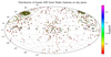Fig. 1.

Sky distribution of all the known GRGs from 1974 to 2020 together with our SAGAN GRG sample in an Aitoff projection. The total number of GRGs plotted here is 820 (LoTSS: 225 and SAGAN: 162, and all others from literature: 433). The large clustering of GRGs in the northern region of the plot (right ascension 10^h45^m to 15^h30^m and declination 45° 00′ to 57° 00′) is the result of finding the large sample of GRGs (225) in the LoTSS by us (Dabhade et al. 2020). The colour of the points on the plot corresponds to their redshift, which is indicated in the vertical colour bar at the right side of the plot. We do not use all the 820 GRGs for our analysis in this paper, but only those (762 GRGs) with a redshift lower than 1.

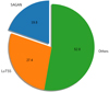Fig. 2.

Pie diagram representing the contribution of SGS (blue: ∼20%) and LoTSS-GRGs (orange: ∼27%) to the total GRG population. The GRGs reported in the literature until March 2020 are plotted in green. We show all the known (820) sources without any filters.

We point out our analysis here is restricted to 762 out of 820 GRGs (∼93% of the GRG catalogue), and 58 GRGs with z > 1 were not considered to avoid any kind of bias. Beyond a redshift of 1, we are limited because no optical data are available and because the radio source properties (luminosity and size) evolve fast in the early cosmic epoch of z > 1. SGS, which is now part of the GRG catalogue, has all sources with z < 1.

3. Analysis

3.1. Size

The projected linear size of the sources is taken as the end-to-end distance between the two hotspots (peak fluxes) in case of FR-II sources, and for FR-Is, it is the distance between the maximum extents defined by the outer lobes. For the measurement of angular sizes, only the NVSS maps are considered for uniformity. The projected linear sizes of sources are estimated using the following formula, and they are tabulated in Table A.1 (Col. 8):

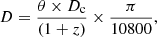
$\begin{matrix} D = \frac{θ \times D_{c}}{(1 + z)} \times \frac{π}{10800}, \end{matrix}$ $\begin{aligned} {D} = \frac{\theta \times D_{\rm c}}{(1+z)} \times \frac{\pi }{10800}, \end{aligned}$ (1)

where θ is the angular extent of the GRG in the sky in units of arcminutes, D_c is the comoving distance in Mpc, z is the redshift of the GRG host galaxy, and D is the projected linear size of the GRG in Mpc.

3.2. Flux density and radio power

The integrated flux density of GRGs was estimated using Common Astronomy Software Applications (CASA; McMullin et al. 2007) with the task CASA-VIEWER by manually selecting the regions of emission associated with each GRG in NVSS⁴ and TGSS⁵ maps. The TGSS maps were convolved to the resolution of NVSS. We used the scheme of Klein et al. (2003) for measuring flux density errors for each source, where we adopted 3% and 20% flux calibration errors, as mentioned in the literature for the NVSS and the TGSS, respectively.

The radio powers of GRGs were calculated using Eq. (2) and are given in Table A.1 (Cols. 10 and 12):

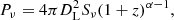
$\begin{matrix} P_{ν} = 4 π D_{L}^{2} S_{ν} {(1 + z)}^{α - 1}, \end{matrix}$ $\begin{aligned} {P}_{\nu } = 4\pi D_{\rm L}^{2}S_{\nu } (1+z)^{\alpha - 1} , \end{aligned}$ (2)

where D_L is the luminosity distance, S_ν is the measured radio flux density at frequency ν, (1 + z)^α − 1 is the standard k-correction term, and α is the radio spectral index (as described in Sect. 3.4).

3.3. Jet kinetic power

AGN jets, made of relativistic charged particles and magnetic fields, emanate from the central engine and pierce the interstellar medium. Low frequency radio observations enable us to estimate the jet kinetic power, which helps us to study other characteristics of the radio-loud SMBH system as discussed in later sections. High radio frequencies (∼1 GHz) are ideal for observing nuclear jet components owing to their flatter spectral nature. Because these components have high velocities, relativistic effects such as the Doppler enhancement effects are prominent. Therefore, lower radio frequencies are more suitable for probing the jet kinetic power because the contribution from Doppler enhancement is negligible. We used the following relation from the simulation-based analytical model of Hardcastle (2018a) to estimate the jet kinetic power:

$\begin{matrix} L_{150} = 3 \times 10^{27} \frac{Q_{Jet}}{10^{38} W} W {Hz}^{- 1}, \end{matrix}$ $\begin{aligned} {L}_{150} = 3 \times 10^{27}\frac{Q_{\rm Jet}}{10^{38}\,W} \mathrm{W\,Hz^{-1}} , \end{aligned}$ (3)

where L₁₅₀ is the radio luminosity at 150 MHz, at which Doppler boosting is negligible, and Q_Jet is the jet kinetic power. There is a scatter of 0.4 dex (rms) about the relation for the sources with z < 0.5. However, significant scatter is observed in the relationship at higher redshifts, with a major contributor being the increased inverse-Compton scattering. Other contributors include the environment and evolutionary state of the sources (Hardcastle 2018a). In the tracks of the P − D diagram for sources of different jet powers in the models presented by Hardcastle (2018a), the luminosity of the source appears to decrease with size during the giant phase for the different jet powers. Their modelling shows that it is possible to obtain more accurate results by taking environment and age into account. The relation is consistent with the regression line of Ineson et al. (2017) and earlier work by Willott et al. (1999).

Sources in the GRG catalogue taken from the Dabhade et al. (2020) GRG sample have flux density measurements at 144 MHz from the LoTSS, which is used to derive the 150 MHz radio luminosity. The TGSS was used for the remaining sources in the GRG catalogue to obtain the 150 MHz radio luminosity. This was mainly done for our newly found SGS, and only sources with full structure detection in TGSS were considered for the same. The results are presented in Col. 8 of Table A.2.

3.4. Spectral index (α)

For a radio source, its spectral index (α) represents the energy distribution of the relativistic electrons (Scheuer & Williams 1968), and its measurement should therefore ideally involve covering wide frequency range. Studies have shown that α correlates with radio power and redshift. For synchrotron radiation, unless it is affected by radiative losses and optical depth effects, it is well known that the radio flux density varies with frequency as S_ν ∝ ν^−α, resulting in a two-point spectral index measurement, given as follows:

$\begin{matrix} α = \frac{ln S_{ν_{1}} - ln S_{ν_{2}}}{ln ν_{2} - ln ν_{1}} \cdot \end{matrix}$ $\begin{aligned} \alpha = \frac{\ln S_{\nu _{1}} - \ln S_{\nu _{2}}}{\ln \nu _{2} - \ln \nu _{1} }\cdot \end{aligned}$ (4)

The integrated spectral index between 150 and 1400 MHz ( $α_{150}^{1400}$ $\alpha^{1400}_{150}$ ) for the GRGs was computed using the TGSS and the NVSS radio maps (Table A.1, Col. 13). We did not include GRGs with incomplete structure detection in the TGSS for the $α_{150}^{1400}$ $\alpha^{1400}_{150}$ studies. For these sources, the $α_{150}^{1400}$ $\alpha^{1400}_{150}$ is assumed to be 0.75 to determine the radio power at 1400 MHz (P₁₄₀₀). See Sects. 4.1 and 5.1.4 for a more detailed discussion.

For sources SAGANJ090111.78+294338.00 and SAGANJ091942.21+260923.97, TGSS data are lacking because they fall in a sky area that is not covered in TGSS-ADR-1. Therefore, no spectral index measurements were possible for them.

3.5. Absolute r-band magnitude

Using the SDSS, we obtained the apparent r-band magnitudes (m_r) of host galaxies of GRGs in the SGS as well as for all the other objects in the GRG catalogue. The absolute r-band magnitudes (M_r) of galaxies were computed after applying the k-correction on extinction-corrected r-band apparent magnitudes (m_r) of SDSS. The k-correction was computed using the K-CORRECT v4.3 software (Blanton & Roweis 2007) for a rest frame at z = 0. Column 5 of Table A.1 shows m_r of the sources from the SGS.

3.6. Black hole mass

We estimated the black hole masses associated with the AGNs in the host galaxies of GRGs using the M_BH–σ relation. The M_BH–σ relation is based on a strong correlation between the central galactic black hole mass (M_BH) and the effective stellar velocity dispersion (σ) in the galactic bulge (Ferrarese & Merritt 2000; Gebhardt et al. 2000) given by

$\begin{matrix} log (\frac{M_{BH}}{M_{⊙}}) = α + β log (\frac{σ}{200 {km s}^{- 1}}), \end{matrix}$ $\begin{aligned} \log \left(\frac{M_{\rm BH}}{M_{\odot }}\right) = \alpha + \beta \log \left(\frac{\sigma }{200\,\mathrm{km\,s}^{-1}}\right) , \end{aligned}$ (5)

where α = −0.510 ± 0.049 and β = 4.377 ± 0.290 (Kormendy & Ho 2013). Estimates for σ (Col. 4 of Table A.2) were available for only 46 host galaxies of GRGs from the SGS in the SDSS, and hence the M_BH of GRGs (Table A.2, Col. 5) could be computed with this method.

3.7. Eddington ratio

The dimensionless Eddington ratio (λ_Edd) is the ratio of the AGN bolometric luminosity to the maximum Eddington luminosity, which in turn is the estimate of the accretion rate of the SMBH in terms of the Eddington accretion rate. The Eddington ratio is expressed by the following relation:

$\begin{matrix} λ \equiv \frac{L_{bol}}{L_{Edd}}, \end{matrix}$ $\begin{aligned} \lambda \equiv \frac{L_{\rm bol}}{L_{\rm Edd}}, \end{aligned}$ (6)

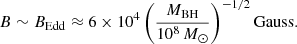
where L_bol represents the bolometric luminosity, and the Eddington luminosity is L_Edd. The L_bol is calculated from the luminosity of the [OIII] emission line using the relation L_bol = 3500 × L_[OIII] (Heckman et al. 2004). The values of λ_Edd are tabulated in Col. 7 of Table A.2. The Eddington luminosity (also known as the Eddington limit) is derived from the black hole mass, and it is the maximum luminosity that an object could have when the force of radiation acting outwards and the gravitational force acting inwards are balanced. The equation of the Eddington luminosity for pure ionised hydrogen plasma is L_Edd = 1.3 × 10³⁸ × ( $\frac{M_{BH}}{M_{⊙}}$ $\frac{M_{\mathrm{BH}}}{{M}_{\odot}}$ ) erg s⁻¹.

3.8. Black hole spin

Spin and angular momentum (a and J) are fundamental properties of black holes, together with the mass. This can help us reconstruct the history of mergers and accretion activity (Hughes & Blandford 2003; Volonteri et al. 2007; King et al. 2008; Daly 2011) that have occurred in the central engine in the past billion years and thus paves the way to understanding the energetic astrophysical jets. In the B − Z model, the relativistic jet is the outcome of the combined effect of rotation (frame dragging) and the accumulated magnetic field near the black hole (Blandford & Znajek 1977), which is fed matter by the rotating accretion disc that surrounds it. In the alternative model of Blandford & Payne (1982), the jet power can come from the rotation of the accretion disc with the help of magnetic threading, without invoking a spinning black hole. However, in both the processes, the intensity and geometry of the poloidal component of the magnetic field near the black hole horizon strongly affect the Poynting flux of the emergent jet (Beckwith et al. 2008).

According to the B − Z model (Blandford & Znajek 1977; Blandford 1990), the relationship between the jet power (Q_Jet), the black hole mass (M_BH), the black hole dimensionless spin (a = Jc/(GM²)), and the poloidal magnetic field (B) threading the accretion disc and ergosphere takes the following form:

$\begin{matrix} Q_{Jet} \propto B^{2} M_{BH}^{2} a^{2}, \end{matrix}$ $\begin{aligned} {Q}_{\rm Jet} \propto B^2 M_{\rm BH}^2 {a}^{2}, \end{aligned}$ (7)

where Q_Jet is in units of 10⁴⁴ erg s⁻¹, B is in units of 10⁴ G, M_BH is in units of 10⁸ M_⊙, and a is the dimensionless spin parameter (a = 0 refers to a non-rotating black hole, and a = 1 is a maximally spinning black hole). The spin (a) can be quantified using the above relation when the other contributing parameters are known or fixed. The constant of proportionality is taken to be $\sim \sqrt{0.5}$ ${\sim}\sqrt{0.5}$ , as in the B − Z model. Owing to the challenges of estimating the magnetic field in the vicinity of the black hole to compute the spin, we considered the Eddington magnetic field strength (B_Edd) (Beskin 2010; Daly 2011), which is

$\begin{matrix} B \sim B_{Edd} \approx 6 \times 10^{4} {(\frac{M_{BH}}{10^{8} M_{⊙}})}^{- 1 / 2} Gauss . \end{matrix}$ $\begin{aligned} {B} \sim B_{\rm Edd} \approx 6 \times 10^{4}\left(\frac{M_{\rm BH}}{10^{8}\,M_{\odot }} \right)^{-1/2} \mathrm{Gauss}. \end{aligned}$ (8)

This is the upper limit of the magnetic field strength close to the central engine, and it is based on the assumption that the magnetic field energy density balances the total energy density of the accreting plasma that has a radiation field of Eddington luminosity. These estimates are presented in Table A.3.

The X-ray reflection is the most robust and effective technique employed to date to estimate the spin of black holes (Reynolds 2019). However, owing to the weakness of the signal and because the data for the objects need to be rich, it has been convincingly performed for only ∼20 sources so far. For radio galaxies, which are jetted sources and mostly show weak X-ray reflection signatures, it is possible to estimate the spin assuming the B − Z mechanism (Daly 2011; Mikhailov & Gnedin 2018). In this radio-driven method, the spin (a) of the black hole can be estimated when we have estimates of M_BH and Q_Jet and adopt B_Edd as B. This method provides an indirect estimate of the spin of the black hole.

3.9. WISE mid-IR properties

We used the WISE survey to study the hosts of GRGs at mid-IR wavelengths. WISE, which is a space-based telescope, carried out an all-sky survey in four mid-IR bands [W1 (3.4 μm), W2 (4.6 μm), W3 (12 μm), and W4 (22 μm)] with an angular resolution of 6.1″, 6.4″, 6.5″, and 12″, respectively.

Using the mid-IR colours, we obtained the properties of possible dust-obscured AGN, and estimated its radiative efficiency. The mid-IR information of host galaxies of GRGs is very useful in gauging the radiative efficiency because the optical-UV radiation from the accretion disc of the AGN is absorbed by the surrounding dusty torus (if present) and is re-radiated at mid-IR wavelengths. Moreover, it has been shown in the literature that WISE mid-IR colours can effectively distinguish AGNs from star-forming and passive galaxies, and within the AGN subset itself, high-excitation radio galaxies (HERGs) and low-excitation radio galaxies (LERGs) stand out in the mid-IR colour-colour and mid-IR-radio plots (Stern et al. 2012; Gürkan et al. 2014). In the absence of any dedicated multi-wavelength survey of host galaxies of GRGs, WISE data are therefore ideal for exploring GRG properties.

The WISE All-Sky Source Catalogue was used to obtain magnitudes of host galaxies of GRGs in the four mid-IR bands. After applying photometric quality cuts of 3σ, we obtained reliable mid-IR magnitudes for sources in the GRG catalogue. Upper limits of the magnitudes in the relevant bands were estimated for sources that did not have a 3σ detection as derived with the method prescribed in the WISE documentation.

Gürkan et al. (2014) have demonstrated that data from WISE can be used to distinguish accretion modes in RLAGNs. To achieve this, Gürkan et al. (2014) used four complete radio samples with emission line-based classification of RGs into low-excitation radio galaxies (LERGs), high- excitation radio galaxies (HERGs), quasars, star-forming galaxies (SFGs), narrow line radio galaxies (NLRGs), and ultra-luminous infrared radio galaxies (ULIRGs). These were further placed in the WISE colour-colour plots, where these sub-classes occupied different regions and thereby enabled distinction. Furthermore, other works (O’Sullivan et al. 2015; Mingo et al. 2016; Whittam et al. 2018) have also confirmed this finding with other radio samples. Therefore we employed the scheme from Mingo et al. (2016), which is based on the earlier work of Wright et al. (2010), Lake et al. (2012), and Gürkan et al. (2014), to classify the host AGN and host galaxies of GRGs into LERGs, HERGs, quasars, SFGs, and ULIRGs.

Figure 3 is a colour–colour plot using four mid-IR bands [W1 (3.4 μm), W2 (4.6 μm), W3 (12 μm), and W4 (22 μm)] and shows not only the distinction between LERGs and HERGs, but also effectively distinguishes AGNs from star-forming and passive galaxies. Figure 3 includes 733 sources from the GRG catalogue based on the availability of data and detection in WISE database. It has been separated into four regions, which signify the following:

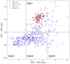Fig. 3.

Position of GRGs and giant radio quasars (GRQs) (733 sources from GRG catalogue) in the mid-IR colour–colour plot using WISE mid-IR magnitudes (W1, W2, W3, and W4 have 3.4, 4.6, 12, and 22 μm Vega magnitudes, respectively). Objects from the GRG catalogue are included. Region I: [W1] − [W2] ≥ 0.5 and [W2] − [W3] < 5.1 is mostly occupied by HERGs and quasars. Region II: objects that have [W1] − [W2] < 0.5 and 0 < [W2] − [W3] < 1.6 are basically LERGs. Region III: star-forming galaxies and LERGs lie mostly in this region ([W1] − [W2] < 0.5 and 1.6 ≤ [W2] − [W3] < 3.4). Region IV: ULIRGs lie in the region of [W1] − [W2] < 0.5 and [W2] − [W3] ≥ 3.4. All the sources have z < 1. The triangle in the plot and the U in the legend indicate the upper limits of the W3 magnitudes.

Region I: HERGs and quasars (W1 − W2 ≥ 0.5, W2 − W3 < 5.1). This region consists of 250 GRGs, 103 of which are hosted by quasars.
Region II: LERGs (W1 − W2 < 0.5, 0 < W2 − W3 < 1.6). This region hosts 153 sources.
Region III: LERGs and star-forming galaxies (W1 − W2 < 0.5, 1.6 ≤ W2 − W3 < 3.4) − 297 giants lie in this region.
Region IV: ULIRGs (W1 − W2 < 0.5, W2 − W3 ≥ 3.4). Only 33 sources lie in this region.

Figure 3 shows that host galaxies of GRGs reveal a variety of AGN excitation types similar to the RG types. This also indicates that the GRG host galaxy or AGN do not preferentially show any specific AGN excitation type. The quasars in this plot are not identified with this method, but were previously classified from the SDSS and other available literature data. Similar results were presented in Dabhade et al. (2017), but with a much smaller sample. We here placed almost the entire GRG catalogue on the WISE colour–colour plot for AGN diagnostic and classified the known GRG population into their excitation types. We focused on the low- and high-excitation part of the classification, and efforts were made to ensure a clean classification. For a sub-sample (based on the availability of data), we also compared our LERG and HERG classification of GRGs from WISE with the standard classification method based on emission line ratios and found them to be consistent with each other.

We refer to the GRGs with low- and high-excitation types as LEGRG and HEGRG, respectively. Because regions III and IV in Fig. 3 both have a mixed population of LERGs as well as star-forming galaxies and ULIRGs, respectively (thereby confusing the classification), we did not consider objects in these regions for our analysis, and considered only sources in region II to be LEGRGs to make a clean sample. Similarly, we excluded from region I known quasars and created a HEGRG sample for our analysis. These two criteria reduce the number of objects available for our further analysis.

4. SAGAN GRG sample: results

The classification of the sources in the SGS is shown in Table 2 below. Out of 162 GRGs, 23 sources are found to be hosted by galaxies with quasars as their AGN (we refer to them as GRQs). The quasar nature of these 23 GRQs is identified using the spectroscopic data from the SDSS, Pâris et al. (2018), and other available literature data. All the GRGs have been detected in the redshift range of ∼0.03−0.95, with projected linear sizes varying from ∼0.71−2.82 Mpc. Three GRGs in our sample have projected linear sizes ≥2 Mpc.

Table 2.

Summary of classified sources.

4.1. Spectral index distribution of the SGS

We were able to estimate $α_{150}^{1400}$ $\alpha^{1400}_{150}$ for a total of 123 from the SGS, 18 of which are GRQs (see Col. 13 of Table A.1). For the remaining 39 sources in the SGS, TGSS had only partial or no detection, and we therefore assumed the spectral index to be 0.75 to calculate P₁₄₀₀. Therefore the $α_{150}^{1400}$ $\alpha^{1400}_{150}$ data for the remaining 39 sources are not included for further studies in this paper. The median value of $α_{150}^{1400}$ $\alpha^{1400}_{150}$ for the GRGs in our sample (0.69 ± 0.02) is similar to that of GRQs (0.69 ± 0.04). Dabhade et al. (2020) also reported that $α_{150}^{1400}$ $\alpha^{1400}_{150}$ of GRGs and GRQs was similar, with almost similar sample size. However, because their sample was chosen from a low-frequency survey such as the LoTSS, they found it to be slighter steeper than our SGS.

4.2. PDzα parameters of GRGs

We investigated the correlation between various properties of sources in our sample, such as radio power (P), projected linear size (D), redshift (z), and spectral index (α) (Fig. 4). The inferences are presented below.

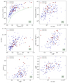Fig. 4.

Correlations of radio power [W Hz⁻¹] at 1400 MHz, size [kpc], redshift, and spectral index for GRGs and GRQs. Red circles indicate GRQs, and blue circles indicate GRGs. The dashed green line in panel a represents the minimum radio luminosity corresponding to a flux density ∼24 mJy of source SAGANJ090640.80+142522.97 at different redshifts, assuming a spectral index of 0.75.

Radio power (P) versus redshift (z): Fig. 4a represents the distribution of GRGs in the P − z plane, with the radio power spanning over three orders of magnitude up to a redshift range of ∼0.95. Most of the sources are within the redshift range of 0.1−0.5, and the number of radio sources decreases with increasing redshift beyond z = 0.5. The non-availability of sources in the lower right quadrant is most likely due to the non-detection of low powered sources at high redshift because of the sensitivity limit of the survey, known as the Malmquist bias. The GRQs occupy the high radio luminosity and high-redshift regime because more optical data are available than for GRGs. The weakest source in our sample is SAGANJ090640.80+142522.97, with a flux density of ∼24 mJy at 1400 MHz. The dashed line represents the minimum luminosity at different redshifts, corresponding to a minimum flux density of ∼24 mJy assuming a spectral index of 0.75. This is the NVSS limit for detecting objects with low surface brightness, and hence the absence of any source below this line. Recently, Dabhade et al. (2020) discovered a large sample of new GRGs, and significant fractions of them were of low luminosity. When we place them on Fig. 4a, they tend to lie below the sensitivity line of NVSS, implying higher sensitivity of LoTSS.
Radio power (P) versus projected linear size (D): The projected linear sizes of the radio sources are plotted against their radio power, measured at 1400 MHz, as shown in Fig. 4b. This plot is the radio astronomer’s equivalent of the traditional Hertzsprung-Russell diagram and is commonly known as the P − D diagram. We can draw the following conclusions from this diagram: – Despite the systematic search for giants, very few sources are found to be of extremely large size and very low radio power (≤10²⁴ W Hz⁻¹ at 1400 MHz). – The upper right region of PD diagram, that is, the region of sources with high radio power and large projected linear size, is devoid of any source. This is indicative of an increase in radiative losses as the sources grow, which decreases the surface brightness and renders them inaccessible to the surveying telescope because of its sensitivity limit. – There is a sudden drop in the number of giants with a projected linear size beyond 2 Mpc. The projected linear sizes of only three sources, SAGANJ064408.04+104341.40, SAGANJ225934.13+082040.78, and SAGANJ231622.32+224650.28 in our sample, exceed 2 Mpc. All of them have low redshifts; the highest is 0.405 for source SAGANJ225934.13+082040.78. The projected linear size of only 66 of ∼762 known GRGs from the GRG catalogue (z < 1) is greater than 2 Mpc. Among them, four sources have extraordinary large projected linear sizes between 3 and 4 Mpc, while another four sources have projected linear sizes ≥4 Mpc, and the largest GRG known to date spans up to 5.2 Mpc at a redshift of 0.3067 (Machalski et al. 2008). About 50% of the sources are at low redshifts (z ≤ 0.4), and the high-redshift objects are mostly dominated by quasars. This might be attributed to the sensitivity limit of radio surveys. Another possibility might be the limited lifetime of radio sources (Schoenmakers et al. 2001). A large fraction of sources may have switched off before they reach 2 Mpc and beyond.
Projected linear size (D) versus redshift (z): Fig. 4c shows the positive correlation between projected linear sizes of our sources with redshift (z < 1), which is expected because luminosity strongly correlates with these two parameters. This may be an outcome of the selection bias of the sources considered in this plot. A negative correlation between projected linear size and redshift is expected from the systematic increase in density of the environment at earlier epochs.
Radio power (P) versus spectral index (α): Fig. 4d shows that the spectral index increases with radio power. The correlation is significant for our sources, which are selected at high frequency (1400 MHz), similar to the results of Laing & Peacock (1980) for extended sources. It is also consistent with results of Blundell et al. (1999), who reported that the spectra of hotspots in powerful radio sources are steeper than those in weaker radio sources. Sources with high Q_Jet form powerful hotspots with enhanced magnetic fields (Blundell et al. 1999), which in turn leads to the rapid synchrotron cooling of relativistic electrons (cooling time τ ∝ 1/B²). This eventually results in an increase in synchrotron losses, and thus electrons with a steeper energy distribution are injected into the lobes.
Redshift (z) versus spectral index (α): Fig. 4e shows that at higher z, we obtain relatively steeper α, although there is a large scatter and sources with steep spectra are also seen at low redshifts. In a flux-density limited sample where luminosity and redshift are strongly correlated, it is difficult to determine whether the primary dependence is on luminosity or redshift (e.g. Blundell et al. 1999). In addition to the effects discussed above, other suggested explanations for the z–α correlation are as follows: – At higher redshifts, the circum-galactic medium is denser, which slows the hotspots down. The hotspots along with the lobes therefore remain in the high-pressure medium for a prolonged duration. A reduction in the velocity will result in the production of electrons with steeper energy distribution (Kirk & Schneider 1987; Mangalam & Gopal-Krishna 1995; Athreya & Kapahi 1998; Klamer et al. 2006; Gopal-Krishna et al. 2012). – In addition to higher synchrotron radiative losses due to a higher magnetic field in the more luminous sources, an important factor at high redshifts is inverse-Compton losses. As the redshift increases, there is a rapid increment in the energy density of the cosmic microwave background radiation (CMBR energy density ∝(1 + z)⁴). When the high-energy electrons of plasma interact with the CMBR photons, energy loss due to inverse Compton radiation increases, and thus the spectra steepen (Krolik & Chen 1991; Athreya & Kapahi 1998; Morabito & Harwood 2018).
Spectral index (α) versus projected linear size (D): The sampling of the sources in the D–α plane in Fig. 4f shows a weak correlation between the two parameters. The larger the sources, the steeper their spectral index. As the sources grow, they are subjected to radiative losses and thereby steepen the energy distribution. However, it is also reflected in the plot that sources with large projected linear size need not have steep spectra. This result is consistent with the findings of Blundell et al. (1999).

4.3. Morphology of GRGs

Using combined information from the VLASS, FIRST, NVSS, and TGSS, we classified the GRGs in our sample into the following types: FR-I, FR-II, HyMoRS, and DDRG. HyMoRS are RGs with a hybrid morphology (Gopal-Krishna & Wiita 2000, 2002) that exhibit an FR-I morphology on one side and an FR-II morphology on the other side of the radio core. The earliest example of this class of objects was presented in Saikia et al. (1996). This classification is listed in Col. 15 in Table A.1, where HM refers to GRGs that are candidates for HyMoRS. Higher resolution radio maps are needed to confirm the morphology of the four HyMoRS candidate GRGs. For HyMoRS candidates, the radio power range is P₁₄₀₀ ∼ 2.74 × 10²⁴ W Hz⁻¹–7.78 × 10²⁵ W Hz⁻¹. The most significant result is that about 92% of the GRGs in the SGS show an FR-II type (edge-brightened hotspots within radio lobes) radio morphology, whereas only 8 out of 162 the GRGs show an FR-I type radio morphology. The radio power (P₁₄₀₀) for FR-I type GRG ranges from ∼1.31 × 10²⁴ W Hz⁻¹ to 11.1 × 10²⁵ W Hz⁻¹, and for FR-II type GRGs. the range extends from ∼0.5 × 10²⁴ to 8.6 × 10²⁶. Recently, Dabhade et al. (2020) used the LoTSS and also found a similar result: most of the GRGs had an FR-II type morphology. Moreover, Mingo et al. (2019) used the LoTSS and reported a significant overlap in radio power of FR-I and FR-II type RGs, along with a new sample of low-luminosity FR-II type RGs.

4.4. Environmental analysis of the SGS

We cross-matched the SGS with one of the largest catalogues of galaxy clusters, the WHL catalogue (Wen et al. 2012). We found 18 GRGs from the SGS that were listed as brightest cluster galaxies (BCGs); they are listed in Table A.4. The mass (M₂₀₀) and virial radius (r₂₀₀) of the clusters were obtained from Wen et al. (2012) and are listed in Table A.4 for these 18 GRGs. The size is expressed as r₂₀₀, which is the radius within which the galaxy cluster mean density is about 200 times the critical density of the Universe, and the mass of the cluster within r₂₀₀ is denoted by M₂₀₀. We considered the sizes of these 18 GRGs along with 111 non-BCG-GRGs from our sample in the same redshift range (0.063−0.369) with median redshifts of 0.174 and 0.205, respectively. We find that the median values for sizes of BCG-GRGs and non-BCG-GRGs are 0.92 Mpc and 1.03 Mpc, respectively. Even though the median values do not vary largely, this indicates that BCG-GRGs have smaller sizes than non-BCGs, or in other words, the immediate environment plays an active role in curtailing their growth.

5. GRG catalogue: properties and correlations

We describe the derived properties of GRGs, consisting of 762 sources with z < 1 using the multi-wavelength data. Our multi-wavelength analysis is divided into the following three parts to understand the nature of GRGs, and we investigate the key astrophysical factors governing their growth to megaparsec scales.

We first studied the differences in AGN types of GRGs: Quasars powering giant radio structures (jets and/or lobes) are called GRQs, which constitute less than 20% of the total known GRG population. The aim is to understand the key differences between giants hosted by quasars and non-quasar AGN. Their properties, such as size, P₁₄₀₀, Q_Jet, and $α_{150}^{1400}$ $\alpha_{150}^{1400}$ , are compared and discussed in Sect. 5.1.

Next, we studied the accretion states (LEGRG or HEGRG) of the central nuclei of GRGs: These two sub-classes are investigated and discussed in Sect. 5.2 in the context of their properties, such as size, P₁₄₀₀, Q_Jet, M_r, M_BH, and λ_Edd. Finally, we studied the similarities and dissimilarities between RGs and GRGs: We compared their $α_{150}^{1400}$ $\alpha_{150}^{1400}$ , M_BH, and λ_Edd properties, and the findings are discussed in Sect. 5.3.

To test whether two samples that we compared come from the same distribution, we used the two-sample Kolmogorov–Smirnov (K-S) test (Kolmogorov 1933; Smirnov 1948; Peacock 1983) and the Wilcoxon-Mann-Whitney (WMW) test (Wilcoxon 1945; Mann & Whitney 1947). In these we tested the null hypothesis H₀: the two samples are drawn from the same distribution, against the alternative hypothesis H₁: the two samples are not drawn from the same distribution. A lower p-value provides stronger evidence that the null hypothesis is rejected, or in other words, that the two samples are not drawn from the same distribution.

In addition to these comparative studies, we explored the SMBH properties to understand how several aspects such as mass (M_BH), spin (a), Eddington ratio (λ_Edd), and jet kinetic power (Q_Jet) are related in Sect. 5.4. Lastly, we discuss in Sect. 5.5 the environmental properties of GRGs that are found in clusters of galaxies (BCGs), and explore their relationship with M₂₀₀ and other BCG-RGs.

5.1. Comparison of the properties of GRGs and GRQs

As mentioned earlier, we here only considered GRGs with z < 1 for analysis. The redshift distribution (Fig. 5 top panel) of GRGs and GRQs is not similar (the WMW test p-value is 3.4 × 10⁻¹³ and the K-S test p-value is 2.9 × 10⁻⁷), however, because GRQs extend to higher redshifts than GRGs. The mean and median redshifts of GRGs are 0.331 and 0.284, respectively, for the range of 0.016−0.910, and for GRQs, the values are 0.515 and 0.475, respectively, for the range of 0.085−0.999. In order to ensure that our results are not affected by redshift evolution, we considered a redshift-matched (0.2 < z < 0.8) (Fig. 5 lower panel) sub-sample of GRGs (mean z: 0.42 and median z: 0.40) and GRQs (mean z: 0.44 and median z: 0.43) to compare their properties (Fig. 7). Here, the redshift distributions of both samples are similar (WMW test p-value is 0.14 and K-S test p-value is 0.54), and our comparison analysis of all properties of GRGs and GRQs gives similar results for the not redshift-matched (Fig. 6) and the redshift-matched samples (Fig. 7). We therefore present our analysis for the samples of GRGs and GRQs below. The detailed statistics of all properties are presented in Table 3.

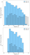Fig. 5.

Redshift (z) distributions of GRGs and GRQs for z < 1, represented in unhatched and hatched bins, respectively for redshift matched (lower plot) and unmatched (upper plot) samples.

Fig. 6.

Distributions of the unmatched sample of GRGs and GRQs with their different properties, represented in not-hatched and hatched bins, respectively, in the redshift range of 0.01 < z < 1.0. The mean and median values of the distributions are given in Table 3. Panel a: size distribution. Panel b: distribution of the radio power at 1400 MHz (P₁₄₀₀). Panel c: distribution of the jet kinetic power (Q_Jet). Panel d: spectral index ( $α_{150}^{1400}$ $\alpha_{150}^{1400}$ ) distribution.

Fig. 7.

Redshift-matched sample of GRG and GRQs in the redshift range of 0.2 < z < 0.8. The description is same as for Fig. 6.

Table 3.

Mean and median values of the properties of the sources in the GRG catalogue for comparison between their sub-types like GRG-GRQ, HEGRG-LEGRG, and GRG-RG.

5.1.1. Distribution of the projected linear size

The distributions of the projected linear size are shown in Figs. 6a and 7a, and the median values are presented in Table 3. Although the median value for quasars appears to be marginally higher when all objects with z < 1 in the GRG sample are considered, the difference is reduced and is within 1σ when the samples are matched in redshift. However, because the GRG sample has been compiled from multiple heterogeneous sources, we also considered the homogeneous samples of the LoTSS and SGS with matched redshifts of GRGs and GRQs. For these two samples, the median values of sizes for GRGs are 0.89 and 1.20 Mpc, and for GRQs, they are 1.00 and 1.06 Mpc, respectively. The WMW test (p-value for the SGS: 0.06, and for the LoTSS: 0.18) shows that the distributions of the projected linear size of GRQs are not significantly different from those of GRGs.

5.1.2. Distribution of the radio power (P₁₄₀₀)

Based on the availability of data from the NVSS, we were able to estimate P₁₄₀₀ for 604 GRGs and 118 GRQs from the GRG catalogue. The distributions of P₁₄₀₀ of GRGs and GRQs are shown in Figs. 6b and 7b for not matched and matched samples, respectively, where we observe that GRQs have a higher radio power than GRGs at 1400 MHz. This is well supported by the K-S test (the p-value for the matched sample is 1.20 × 10⁻⁷) and the WMW test (the p-value for the matched sample is 7.88 × 10⁻¹¹) of the matched redshift samples, as shown in Table 3, which strongly indicates that the two distributions are significantly different. Clearly, prevailing conditions in the central engines of GRQs are able to produce more powerful jets, which results in more radio-luminous sources than for GRGs. GRQs are found to have a higher jet kinetic power than GRGs (as shown below), and they might host more massive black holes that accrete at a higher Eddington rate. Because our sample is restricted to sources with redshift lower than 1, we do not observe even more powerful GRQs, which lie mostly at higher redshifts.

5.1.3. Distribution of the jet kinetic power (Q_Jet)

The Q_Jet of the GRGs and GRQs was estimated using TGSS and the LoTSS, as explained in Sect. 3.3. Figures 6c and 7c show the histograms of Q_Jet of GRGs and GRQs. It it is evident that the GRQs have higher values of Q_Jet, which is also supported by the statistics presented in Table 3. From the inverse correlation between jet power and dynamical age, that is, Q_Jet ∝ 1/ $t_{age}^{- 2}$ $t^{-2}_{\mathrm{age}}$ (Ito et al. 2008), it can be inferred that if their sizes are similar, more powerful radio jets of the GRQs would take less time in scaling Mpc distance than the GRGs (if they are placed in an environment of similar ambient density, which is not clear at this stage). Using a sample of 14 GRGs, Ursini et al. (2018) also reported that Q_Jet of GRGs lies in the range of ∼10⁴² erg s⁻¹ to 10⁴⁴ erg s⁻¹. It has been observed (Mingo et al. 2014) that some RGs have far higher Q_Jet than GRGs, which could be attributed to the severity of the radiative losses suffered by the GRGs over a period of their growth.

Ursini et al. (2018), based on their Fig. 3, hypothesised that GRGs like RGs at the start of their life have high nuclear luminosities as well as high Q_Jet, which eventually fades over a period of time. Because their sample of GRGs was hard X-ray selected, it also shows high nuclear luminosities, and other GRG samples (such as our GRG-catalogue sample), which are radio selected, will occupy the lower luminosity part of Fig. 3 in Ursini et al. (2018). Our findings based on the GRG catalogue support their hypothesis, as we mostly have radio-selected GRGs with L_bol in the range of ∼10⁴² erg s⁻¹ to 10⁴⁶ erg s⁻¹, which extends below the L_bol range of the Ursini et al. (2018) hard X-ray selected sample of 14 GRGs.

5.1.4. Distribution of the spectral index ( $α_{150}^{1400}$ $\alpha_{\mathsf{150}}^{\mathsf{1400}}$ )

Figures 6d and 7d shows the histograms of the spectral indices of GRGs and GRQs. A similar criterion (as mentioned in Sects. 3.4 and 4.1) of considering only those sources that are fully detected in TGSS (or LoTSS) and NVSS was followed for the sources in the GRG catalogue. The mean value, median value, and the p-values of the K-S and WMW tests (Table 3) confirm that the GRGs and GRQs have the same distribution of the spectral index. This result is also consistent with the recent findings of Dabhade et al. (2020).

5.2. Comparison of the properties of HEGRGs and LEGRGs

Based on the criteria mentioned in Sect. 3.9, we classified the GRGs into high- and low-excitation, or HEGRGs and LEGRGs, types. When we consider their respective RG counterparts, called LERGs and HERGs, the LERGs are the dominant population as compared to HERGs. About 12% of the sample of Kozieł-Wierzbowska & Stasińska (2011) are HERGs, and is similar for Best & Heckman (2012). As mentioned previously in Sect. 3.9, in order to have a clean sample, we did not consider LERGs or LEGRGs from region III as they are contaminated with possible star formation. Therefore, our LEGRG sample is drastically reduced to 153 because we only considered sources from region II to be LEGRGs. Region I includes 147 HERGs and therefore makes our comparison samples almost equal with each other. In the following subsections, we individually describe the distribution of HEGRGs and LEGRGs in terms of various properties.

The redshift distributions of the HEGRGs and LEGRGs are shown in Fig. 8 (upper panel). Their redshifts lie in the range 0.02 < z < 0.89. We note that the redshift distributions are not the same, and we therefore considered two sub-samples matched in redshifts, whose details are described below.

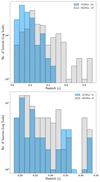Fig. 8.

Redshift (z) distributions of LEGRGs and HEGRGs for 0.02 < z < 0.89 (unmatched redshift), represented in not-hatched and hatched bins, respectively in the upper plot. Similarly, in lower plot distributions are shown for matched redshift high-z: 0.18 < z < 0.43 sample of LEGRGs and HEGRGs.

Low-z: The first sub-sample consists of 27 HEGRGs and 93 LEGRGs in the matched lower redshift range of ∼0.04 to 0.18. The HEGRGs and LEGRGs have similar mean (LEGRGs: 0.12, and HEGRGs: 0.11) and median (LEGRGs: 0.11, and HEGRGs: 0.10) redshift values as well as the same distribution (K-S test p-value: 0.52 and WMW test p-value: 0.19).

High-z: As shown in Fig. 8 (lower), the second sub-sample consists of 87 HEGRGs and 53 LEGRGs in the matched higher redshift range ∼0.18 to 0.43. They have similar mean (LEGRGs: 0.26, and HEGRGs: 0.27) and median (LEGRGs: 0.24, and HEGRGs: 0.25) redshift values as well as the same distribution (K-S test p-value: 0.47 and WMW test p-value: 0.23).

All three samples of HEGRGs and LEGRGs, that is, the total sample, high-z, and low-z, give similar results in the comparison of their different properties. Therefore, below, we present the results of the total sample and of the high-z sample of HEGRGs and LEGRGs. Figures 9 and 10 show that for each property, the number of sources vary because it is dependent on the availability of data from public archives such as the SDSS, NED, and Vizier.

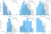Fig. 9.

Distributions of LEGRGs and HEGRGs according to their various physical properties. They are represented in not-hatched and hatched bins, respectively, in the redshift range of 0.01 < z < 1.0. The mean and median values of the distributions are given in Table 3. Panel a: distribution of the physical size (Mpc). Panel b: distribution of the radio power at 1400 MHz (P₁₄₀₀). Panel c: distribution of the jet kinetic power (Q_Jet). Panel d: distribution of the absolute r-band magnitude (M_r). Panel e: distribution of the black hole mass (M_BH). Panel f: distribution of the Eddington ratio (λ_Edd).

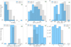Fig. 10.

Redshift-matched samples of LEGRGs and HEGRGs in the range 0.18 < z < 0.43. The description is same as for Fig. 9.

5.2.1. Distribution of the projected linear size

The projected linear size distributions of LEGRGs and HEGRGs from the GRG catalogue for unmatched and matched redshift samples are shown in Figs. 9a and 10a, respectively. Both classes seem to follow different distributions, as indicated by the p-values of the K-S and WMW tests, as shown in Table 3. Our data suggest that HEGRGs tend to grow to larger sizes than the LEGRGs, as seen from their mean and median sizes presented in Table 3 for both samples. In other words, the radiatively efficient nature of HEGRGs helps GRGs to grow to larger sizes.

Similarly, when we take a sample of RGs (∼400 RGs; Kozieł-Wierzbowska & Stasińska 2011) for which we have size estimates along with a high- and low-excitation classification (from WISE), we find a similar result: the sizes of high-excitation sources (HERGs) are larger than those of low-excitation sources (LERGs). This particular property is clearly similar for RGs and GRGs and is independent of the overall size of the source.

5.2.2. Distribution of the radio power (P₁₄₀₀)

Figures 9b and 10b show P₁₄₀₀ distributions of LEGRGs and HEGRGs for unmatched and matched redshift samples, respectively. Based on these, we infer that the HEGRGs spread over a larger range of P₁₄₀₀ than LEGRGs. The distributions are different, as is strongly indicated by the p-values of the K-S and WMW tests. Their distributions also overlap significantly, with HEGRGs having higher P₁₄₀₀ than LEGRGs, as shown in Table 3. This result complements the fact that HEGRGs are in a high-accretion state, resulting in the high radio power of GRGs. Kozieł-Wierzbowska & Stasińska (2011) also found that HERGs, like HEGRGs, which are radiatively efficient, have a higher radio power at 1400 MHz.

5.2.3. Distribution of the jet kinetic power (Q_Jet)

The Q_Jet of both the populations varies over a wide range, with HEGRGs occupying the higher end of the distributions, as shown in Figs. 9c and 10c. The difference in Q_Jet is statistically significant; the median Q_Jet ∼ 10⁴⁴ erg s⁻¹ of HEGRGs is about ten times higher than that of LEGRGs (Table 3). The high mean and median values of HEGRGs (as shown in Table 3) compared to LEGRGs strongly indicate that the AGNs of GRGs with high-excitation type are responsible for launching higher powered jets, resulting in more radio-luminous sources (higher P₁₄₀₀ as above).

5.2.4. Distribution of the absolute r-band magnitude (M_r)

The distributions of M_r in unmatched and matched redshift bins of LEGRGs and HEGRGs are presented in Figs. 9d and 10d. These figures show two distinct populations, and this is also supported by the low p-value of the K-S and WMW tests (Table 3). The LEGRGs are found to be optically brighter by ∼1 mag than HEGRGs, indicating that LEGRGs are mostly hosted by bright giant elliptical galaxies comprising an old stellar population, which is quite prominently visible from their absolute r-band magnitudes. This is consistent with the findings of Hardcastle et al. (2007), who have shown this for LERGs.

Overall, Figs. 9d and 10d show the M_r distribution of GRGs, which ranges from ∼−19 to −25 in brightness. A similar distribution has been observed for host galaxies of normal-sized RGs (Govoni et al. 2000; Sadler et al. 2007; Capetti et al. 2017).

5.2.5. Distribution of the black hole mass (M_BH)

A study of the M_BH distribution in LEGRGs and HEGRGs is very crucial for understanding one of the key factors driving the two different accretion modes. For this study, our sample was restricted to 94 sources (unmatched redshift sample) based on the availability of the spectroscopic data from the SDSS. Figure 9e (unmatched redshift sample) and Fig. 10e (matched-redshift sample) show the distributions of M_BH in these two classes, in which the mean and median (see Table 3) of LEGRGs are found to be greater than HEGRGs. The higher values of mean and median of the M_BH of LEGRGS compared to HEGRGs as well as the low p-value of the K-S and WMW tests implies that HEGRGs have lower M_BH than LEGRGs.

5.2.6. Distribution of the Eddington ratio (λ_Edd)

In this study, the sample was restricted to just 55 (unmatched redshift sample) because of the availability of reliable [OIII] line flux data from the SDSS, which is essential for estimating the L_bol. Out of this, a total of 48 GRGs are classified as LEGRG, and 7 are classified as HEGRG in the GRG catalogue based on their mid-IR properties. Nearly 87% of the sample are LEGRGs, which is consistent with earlier studies (Hardcastle 2018b), which showed that LERGs are the dominant population of radio galaxies. LERGs or LEGRGs are dominated by the radiatively inefficient accretion flow, or RIAF (Yuan & Narayan 2014). In Figs. 9f and 10f we observe the distribution of the λ_Edd, which ranges from ∼10⁻⁴ to 10⁻² for LEGRGs and from 10⁻² to 10⁻¹ for HEGRGs, with a little overlap. The lower λ_Edd values of (Table 3) of LEGRGs implies a radiatively inefficient state governed by a low accretion rate. HEGRGs, in contrast to LEGRGs, are rarer and have a comparatively higher λ_Edd (Table 3), indicating their radiatively efficient mode and higher accretion rate. Our results for GRGs are similar to previous findings for RGs by Kozieł-Wierzbowska & Stasińska (2011), Smolčić (2009), and Best & Heckman (2012), who have shown that λ_Edd is higher for HERGs than for LERGs. The λ_Edd of LEGRGs peaks around 10⁻⁴, which is consistent with the findings presented in Ho (2008).

5.2.7. HEGRG-LEGRG comparison overview

In the six subsections above we compared HEGRGs to LEGRGs by comparing several properties of LEGRGs and HEGRGs in the total sample as well as redshift-matched ones. The results are similar: (a) The HEGRGs tend to be larger, more luminous, and have a higher jet power than LEGRGs, (b) LEGRGs are optically brighter by ∼1 mag than HEGRGs, (c) LEGRGs have lower Eddington ratios, harbour higher mass black holes, and launch lower power jets (by a factor of 10) than HEGRGs. This implies that higher mass black holes grow in the nucleus of optically brighter and more massive galaxies, whose central engines are presently found in low-excitation, radiatively inefficient, low mass accretion state but are capable of producing sufficiently powerful FR-II jets that result in Mpc-scale GRGs, which clearly constitute the vast majority (> 80%) of all GRGs selected in our study. Although it is beyond the scope of this work, it will be useful in future when the detailed properties of LERGs are compared with LEGRGs and HERGs with HEGRGs in order to gain much deeper insight into the inner workings of the GRG central engine.

5.3. How similar are GRGs and RGs?

The following studies were carried out to understand the factors that cause a very small population of RGs to transform into GRGs. We carried out this investigation by studying three of their properties: α, M_BH, and λ_Edd, in this section. Possible differences in black hole spin and their implications are discussed in Sect. 5.4.1.

5.3.1. Spectral index (α)

Several radio spectral index studies of RGs (Kellermann et al. 1969; Oort et al. 1988; Gruppioni et al. 1997; Kapahi et al. 1998; Sirothia et al. 2009; Ishwara-Chandra et al. 2010; Mahony et al. 2016) have established the mean spectral index value to be ∼0.75. Until recently, it was believed that GRGs have steeper spectral index values. However, Dabhade et al. (2020), using their large sample of GRGs, found that the spectral index of RGs and GRGs is very similar. Now, with our GRG catalogue (which comprises of LoTSS and SGS), we establish this result strongly with a larger (> 250) sample size, as shown in Table 3: the mean α for GRGs and GRQs is ∼0.75 and ∼0.72, respectively, for the unmatched redshift sample. For the matched-redshift sample, the mean α for GRGs and GRQs is 0.77 and 0.70, respectively. These values are similar to those of the RGs and RQs.

5.3.2. Black hole mass (M_BH)

Here, in the first point we describe how we derived the redshift matched RG sample for comparison along with its properties. In the second point we describe our sub-sample of GRGs derived from the GRG catalogue. Lastly, in the third point we present the result of our comparative study.

1. RG sample. In order to compare the M_BH of GRGs and RGs, we used the RG sample from Best & Heckman (2012). This RG sample was created using the SDSS DR7 (Abazajian et al. 2009) optical spectroscopic data along with the FIRST and NVSS radio data. This sample has been filtered from star-forming galaxies (SFGs) and only consists of radio-loud AGNs (RLAGNs) or RGs. Furthermore, we used their stellar velocity dispersion (σ) information to compute M_BH from the SDSS DR14 database (Abolfathi et al. 2018) through CasJobs⁶, and retained only galaxies with reliable spectra, that is, a redshift warning flag, ZWarning = 0, from the SDSS DR14 database. Next, only sources with σ in the range of 80 < σ < 420 km s⁻¹ were selected based on the criterion provided by Bolton et al. (2012). Lastly, in order to have a more clean and robust sample, we also imposed an additional filter to the sources in the sample to have a σ error smaller than 30%. The redshift range of the RG sample was restricted to the range of 0.034 to 0.534 to match the redshift range of the GRG sample (from the GRG catalogue) used for this study (see below), and radio-loud quasars were not considered for this study. This reduced the original RG sample of Best & Heckman (2012) to 14543. We call this sample as BH12 in the remainder of the paper.

2. The GRG sample. In our SGS, only 46 GRGs have spectroscopic data from the SDSS, and only these therefore have M_BH estimates derived from the M_BH–σ relation. In order to carry out a comparative study of M_BH that is statistically significant, we make use of the GRG catalogue. Out of 820 GRGs in the GRG catalogue (including the SGS), 164 have clean, reliable σ information from the SDSS. For the purpose of the M_BH RG-GRG comparison study, our sample of GRGs was therefore restricted to 164.

3. Distribution of the black hole mass. Figure 11a shows that the distributions of RGs and GRGs are largely similar. The spread of RGs is wider at the lower end of the plot than for GRGs, but both distributions peak at a similar value and have similar mean and median values (GRG: mean = 1.04 × 10⁹ M_⊙, and median = 0.84 × 10⁹ M_⊙; RG: mean = 1.10 × 10⁹ M_⊙, and median = 0.84 × 10⁹ M_⊙). This establishes that both RGs and GRGs have the same M_BH distribution, and it is also supported by the K-S and WMW tests, where the p-values are 0.86 and 0.46, respectively.

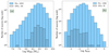Fig. 11.

Distribution of black hole mass (M_BH) in panel a and Eddington ratio (λ_Edd) in panel b of RGs (not-hatched bins) and GRGs (hatched bins). The RG sample has been derived from Best & Heckman (2012) and the GRG sample is from the GRG catalogue created by us.

5.3.3. Eddington ratio (λ_Edd)

Based on the availability of the [OIII] line flux information from the SDSS, we have the estimates of λ_Edd for 99 GRGs from the GRG catalogue and 12998 RGs from BH12, whose distribution is shown in Fig. 11b. Based on our analysis of the available data, it appears that the RGs and GRGs have different mean and median values (Table 3). The plot shows that the distributions are different, which is statistically evident from the p-value of 2.78 × 10⁻¹⁴ from K-S test and from the p-value of 1.38 × 10⁻¹⁴ from the WMW test. Thus, our data indicate that λ_Edd of RGs is higher than that of GRGs. We can further extrapolate and conjecture that GRGs mostly have RIAF as compared to RGs, as almost all the GRGs have λ_Edd < 0.01 (which is the RIAF regime).

5.4. Astrophysical processes near accreting black holes in GRGs

In this section we discuss the black hole properties of GRGs based on our estimates of spin, Eddington ratio and jet kinetic power. We also present the possible astrophysical scenarios leading to the observed properties of GRGs.

5.4.1. Black hole spin (a)

The spin of the accreting black hole has been identified as one of the key ingredients for powering the relativistic jets in AGN for a timescale of millions of years or more. Spin is coupled with the strength and geometry of the magnetic field, and by rearranging Eq. (7), we obtain

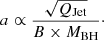
$\begin{matrix} a \propto \frac{\sqrt{Q_{Jet}}}{B \times M_{BH}} \cdot \end{matrix}$ $\begin{aligned} {a} \propto \frac{\sqrt{Q_{\rm Jet}}}{{B} \times M_{\rm BH}}\cdot \end{aligned}$ (9)

The spin (a) of the black hole of GRGs was estimated using our M_BH and Q_jet estimates, as explained in Sect. 3.8 and given in Table A.3. We emphasise here that these are crude estimates based on certain assumptions. We rejected sources with an error of 60% and higher in their M_BH estimates, and our sample (GRG catalogue) was therefore restricted to 95 sources for this particular study, as listed in Table A.3. Figure 12 shows the distribution of black hole spin with respect to M_BH varying over two orders of magnitude, that is, 10⁷ to 10⁹ M_⊙. The spin range spans from 0.007 to 0.518, resulting in mean and median values of 0.079 and 0.055, respectively, for GRGs in our sample. We also plot iso-tracks with their respective colours, which indicate the constant jet kinetic powers obtained for various ranges of spin, M_BH, and magnetic field strength.

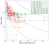Fig. 12.

Simulation of black hole spin (using Eq. (9)) as a function black hole mass over various ranges of jet kinetic power. Coloured points represent estimated values from GRG observations. The solid curved lines with their respective colours indicate the different values of spin attainable by a black hole for a mass range of 10⁷ M_⊙ to 10⁹ M_⊙ at that particular jet kinetic power. The solid circles with different colours indicate the GRGs in our sample with their estimated spin values lying in the range of jet kinetic power specified. The total number of GRGs is 95. Figures mentioned in the square brackets in the legend of the plot indicate number of GRGs in respective kinetic jet power bins. The magnetic field used to compute the black hole spin (a) was assumed to be B_Edd, which is derived from the M_BH.

Figure 12 shows distribution of spin as a function of black hole mass in various bins of Q_Jet from 10⁴¹ erg s⁻¹ to 10⁴⁵ erg s⁻¹, which we simulated using Eqs. (7) and (8). With the plausible values of black hole mass, magnetic field, and spin, clearly no GRG is observed to acquire a Q_Jet ≥ 10⁴⁵ erg s⁻¹. For the objects with a low value of Q_Jet (∼10⁴¹ erg s⁻¹), even a drastic change in the magnetic field or M_BH would lead to only a minute change in spin, whereas for the objects with higher Q_Jet (∼10⁴⁴ erg s⁻¹) values, a small change in the magnetic field or M_BH would result in a significant change in spin values. Based on our sample, we observe that the spin values of 99% of GRGs are constrained within 0.3. For the source with the highest spin value of 0.518, a correct combination of lower mass and high jet power as compared to the rest of the sources served as a favourable condition. AGNs of both types, that is, with and without powerful jets, have SMBHs that spin rapidly, which in turn implies that spin alone is not the driving factor for the production of powerful relativistic jets. Our spin estimates are based on assuming the maximum possible magnetic field, that is, B_Edd, which indicates that these are the lowest possible values. Below we discuss the implications of this result, which is a possible scenario for GRGs.

King & Pringle (2006) reported that if a black hole has a series of accretion episodes whose principal angular momentum vectors are randomly orientated (a chaotic random-walk process), in which the black hole angular momentum dominates, then it leads to lower black hole spin values. However, the successive accretion flows accumulate the poloidal magnetic flux in the vicinity of the black hole, and this strong magnetic flux threading the black hole accretion disc might lead to the state of a magnetically arrested disc (MAD), which affects the dynamical accretion process onto the black hole itself (Narayan et al. 2003; Tchekhovskoy et al. 2011). This state disrupts the accretion flow by breaking the flow into small streams. The velocity of the stream decreases with respect to free-fall velocity as the material in the stream has to find its way to the black hole through magnetic interchange and reconnection, which results in lower spin values of the black hole. Similarly, the low spin value of GRGs can be explained when we invoke the state of MAD, or equivalently, a dynamically important magnetic field B_dyn, which indicates that their accretion history was chaotic rather than a smooth, progressive process. The dynamically important magnetic field field near the black hole has been observationally shown to exist (Eatough et al. 2013).

Another possible scenario might be self-gravity, which fragments the material in the disc into small clouds with randomly oriented angular momentum (Fanidakis et al. 2011). This leads to randomly oriented numerous accretion episodes that collectively lower the spin of the black hole. The lower spin correlating with higher mass black holes (Fig. 9) suggests that SMBHs powering the GRGs were perhaps formed in episodes of quasi-isotropic chaotic accretion events.

Alternatively, when we assume a maximally spinning (Thorne limit: a = 0.998) black hole (Thorne 1974) for our GRGs, then using our M_BH and Q_Jet estimates of a sample 95 GRGs, we can set a lower limit on their magnetic field strength (B or B_dyn). Thus we obtain the values of B_dyn in the range of 1.1 × 10² < B_dyn < 1.8 × 10⁴ G for our GRGs with the mean value of 2.2 × 10³ G. These limits on B match the limits given using very long baseline interferometry (VLBI) observations of RLAGN, which can probe the parsec to sub-parsec scale region around the black hole (Zamaninasab et al. 2014; Martí-Vidal et al. 2015; Baczko et al. 2016; Hodgson et al. 2017; Boccardi et al. 2017).

5.4.2. Disc-jet coupling: Interplay between Eddington ratio (λ_Edd), spin (a), and jet kinetic power (Q_Jet)

The role of the black hole spin and accretion rate in launching the observed radio jets is still highly contentious and an unsolved issue (Reynolds 2019). Most often, the jet radio luminosity is taken as a good indicator of the jet kinetic power, but in reality, it is only a small fraction of the latter. The question then is what the source of the radio jet power is that we observe in black hole systems that fuels the extremely large GRGs. How its luminosity scales with the black hole spin and accretion rate is another open question.

The growth and evolution of an AGN is coupled with the accretion phenomenon and the spin of the central black hole. In order to understand the possible co-dependence of various parameters of the black holes for the purpose of jet launching and propagation, we studied how λ_Edd affects the Q_Jet. We created a sub-sample of 57 GRGs (based on their data availability) from the GRG catalogue and find a linear correlation between the Eddington ratio (λ_Edd) and Q_Jet/L_Edd (dimensionless jet kinetic power), which is strongly supported by the Spearman correlation coefficient of 0.8, as shown in Fig. 13a. The relation between the two parameters takes the following form: log λ_Edd = 0.81 × log(Q_Jet/L_Edd) − 0.005 based on our data. This implies that L_bol has a significant effect on the collimated kinetic jet output (Q_Jet) of the AGN because $λ_{Edd} = \frac{L_{bol}}{L_{Edd}}$ $\lambda_{\mathrm{Edd}} = \frac{{L}_{\mathrm{bol}}}{{L}_{\mathrm{Edd}}}$ , and the corresponding equation takes the form log L_bol = 0.66 × log(Q_Jet) + 15.38, as evident from Fig. 13b. The Spearman correlation coefficient for this correlation is 0.7.

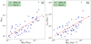Fig. 13.

Panel a: linear correlation for 57 objects between the Eddington ratio (λ_Edd) and the ratio of the jet kinetic power (Q_Jet) to the Eddington luminosity (L_Edd), which can be represented as log λ_Edd = 0.81 × log(Q_Jet/L_Edd) − 0.005, as discussed in Sect. 5.4.2. Panel b: bolometric luminosity (L_bol) as a function of jet kinetic power (Q_Jet), which takes the equation form log L_bol = 0.66 × log(Q_Jet) + 15.38. The Spearman correlation coefficient is 0.8 and 0.7 for panels a and b, respectively. The red line indicates the best linear fit of the correlations in the log–log plots.

The formation and propagation of highly relativistic magnetised jets is dependent (disc-jet coupling) on the magnetic field strength coupled to magnetic field geometry of the accretion disc (McKinney & Narayan 2007). Zamaninasab et al. (2014) have shown that a strong correlation exists between the jet magnetic field ϕ_Jet and the accretion disc luminosity (L_acc or L_bol). Furthermore, they also concluded that the launching regions of jets are threaded by dynamically important magnetic fields with the possible effect of the black hole spin. They strongly favoured the MAD model of the accretion disc. Similarly, Sikora & Begelman (2013) also argued in favour of magnetic flux threading of black hole over spin and Eddington ratio as the governing factor for the launch of collimated powerful radio jets. Zamaninasab et al. (2014) reported that the magnetic flux of the black hole ϕ_BH ∝ $\sqrt{L_{bol}}$ $\sqrt{{L}_{\mathrm{bol}}}$ M_BH, and in absence of direct measurements of ϕ_BH, we can therefore use L_bol as a proxy. Therefore, our L_bol–Q_Jet correlation (discussed above) is also indicative of a strong effect of ϕ_BH on Q_Jet. This strongly indicates a disc-jet coupling phenomenon where the magnetic field in the magnetically arrested disc surrounding the black hole controls the dynamics of accretion flow responsible for the jet launching. A lower magnetic field might therefore also be responsible for the lower Q_Jet, as evident from Fig. 13b, where L_bol acts as a proxy for the magnetic field (ϕ_BH).

In an advection-dominated accretion flow (ADAF, Narayan & Yi 1994), Q_Jet is related to L_Edd (Fanidakis et al. 2011) by

$\begin{matrix} Q_{Jet} \sim 0.01 a^{2} L_{Edd}, \end{matrix}$ $\begin{aligned} {Q}_{\rm Jet} \sim 0.01 {a}^{2}L_{\rm Edd}, \end{aligned}$ (10)

where Q_Jet and L_Edd are in erg s⁻¹. This shows that 1% of L_Edd at most can be converted into Q_Jet when we consider a maximum spin value of 0.998. Based on our analysis, we infer that ∼0.06% of L_Edd on an average is converted into Q_Jet for GRGs. Therefore it is evident from this result and the discussion that for GRGs the fraction of L_Edd that is converted into Q_Jet is quite low. It is therefore expected that the spin values are lower as well. This matches the estimated spin values we presented in Sect. 5.4.1, where the mean spin value is ∼0.079. The spin values for our GRGs were estimated using independently computed Q_Jet and M_BH values. Here, Q_Jet is the lower limit as the Q_Jet relation (Eq. (3)) from Hardcastle (2018a) is expected to underestimate the Q_Jet for GRGs, and the spin values are therefore also expected to be the lower limits. From the correlations shown in Fig. 13a, we expect a significant correlation between the spin and λ_Edd as well, represented in the relation log λ_Edd = 1.62 × log(a) − 1.02 based on the same data. The Spearman correlation coefficient for the above is 0.8.

Based on our results, we observe strong evidence of a tight correlation between the spin and λ_Edd at least for the lower regime of spin and λ_Edd values. Figure 12 clearly shows that the spin value decreases with increasing black hole mass, which is quite consistent with the findings of Daly (2011) and Griffin et al. (2019), but the magnitude of the spin for GRGs is lower than in their sample studies.

Observations (Reynolds 2019) from the X-ray reflection of nearly two dozen SMBHs (prone to bias) have shown that the higher mass black holes (≥10⁸ M_⊙) tend to have low spin (a ≤ 0.7) values, which is quite similar to our results for the GRGs, although our average spins are much lower. It is not ideal to compare properties of an X-ray selected AGN sample (as mentioned in Reynolds 2019) and radio-selected AGN (like our GRGs).

The two correlations as shown in Figs. 13a and b together may explain the effect of magnetic field and spin on the kinetic output of relativistic jets. An increment in spin leads to an increment in λ_Edd, and this eventually enhances the conversion of L_Edd into Q_Jet. In other words, the higher the Eddington ratio, the higher the accumulation of magnetic flux near the black hole. leading to saturation of the magnetic field (MAD). It drives the magneto-rotational instabilities, which carry away the angular momentum of the in-falling material, and thus control the accretion flow. The magnetic flux in the jetted output scales with the magnetic flux threading the black hole. Furthermore, the spin twists the magnetic field lines around the black hole to transfer energy in the form of Poynting flux through jets. The magneto-hydrodynamics and spin of black holes thus play a crucial role in the formation of the powerful jets which could extend to large distances.

5.5. Environment analysis

We used the GRG catalogue to determine how many GRGs might be hosted by BCGs in galaxy clusters. To do this, we used the WHL galaxy cluster catalogue, as done for SGS in Sect. 4.4. We find that a total of 60 GRGs from the GRG catalogue are BCGs, residing in a dense cluster environment. These 60 BCG-GRGs clearly provide strong evidence that sparse environment alone is not responsible for the large size of all GRGs, and powerful AGNs like these can pierce the dense cluster environment to grow to Mpc scales.

In Fig. 14a, we explore the relation between the sizes of the GRGs and the M₂₀₀ of the respective galaxy clusters. We observe that GRGs with sizes ≥1 Mpc are not found in clusters with M₂₀₀ greater than 2.5 × 10¹⁴ M_⊙. Figure 14b shows the distribution of M₂₀₀ of clusters with radio-loud BCGs and BCG-GRGs, where we observe that radio-loud BCGs occur in clusters with a wide range of M₂₀₀. About 95% of the BCG-GRGs in our sample are located in clusters with M₂₀₀ lower than 2 × 10¹⁴ M_⊙. Below we test whether this result is statistically significant. Interestingly, no GRG found to be residing in the cluster environment is observed to grow beyond the virial radius (R₂₀₀) of the host cluster. Also, we do not find a correlation between the total P₁₄₀₀ of the GRGs and the mass of the cluster.

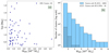Fig. 14.

Panel a: mass of the galaxy cluster hosting the BCG-GRG (x-axis) and size of the GRG (y-axis). Panel b: distribution of M₂₀₀ of clusters with radio-loud BCGs and clusters with GRG as BCGs from the GRG catalogue.

The K-S test on the distributions of M₂₀₀ of BCG-GRGs and radio-loud BCGs gives a p-value of 0.83, which indicates that the two distributions are identical. When we take the ratio of the number of BCG-GRGs to the radio-loud BCGs in the first four mass (M₂₀₀) bins, we obtain 0.0055, 0.0061, 0.0033, and 0.0099, respectively, with an average value of 0.0062. If we assume this ratio to be true for all mass bins, then this indicates that we should expect that only 0.62% of the radio-loud BCGs in clusters are GRGs. The cosmological halo mass function of evolving structures shows that the abundance of low-mass clusters is much higher than the abundance of high-mass clusters in the local Universe (Sheth et al. 2001). Moreover, as the number of high-mass clusters is interestingly very low, we obtain an even lower number of radio-loud BCGs hosting GRGs in the cluster environment. For example, when we take the mass bin around 7 × 10¹⁴ M_⊙ (6th bin), then there are 14 radio-loud BCGs in this bin. The average value of the ratio, 0.0062, suggests that we needed about 160 clusters of such high masses with a radio-loud BCG to detect at least one GRG. Therefore the probability of finding a radio-loud BCG as a GRG in clusters is indeed very low, and it is very difficult to find them in massive clusters.

We also observe that the radio morphology of BCG-GRGs is not linear and symmetric, but is rather deformed to a certain degree. This clearly illustrates the effect of the environment on the GRGs, which, despite the resistance of the intra-cluster medium and cluster weather, are able to grow to megaparsec scales.

In order to study the environment of the GRGs more thoroughly, we need to determine precisely the fraction of the GRG population that resides in clusters (BCG or a cluster member), which can only be achieved with a controlled and complete sample. We will be focusing on this aspect in our future work within project SAGAN.

6. Discussion

Based on our study, we further discuss the overall results in the context of GRGs in this section. Nearly 20-year-old surveys such as the NVSS, when combined with other radio and optical surveys, still have a high discovery potential. This is evident from the large sample (SGS) of 162 GRGs discovered by us, which increases the overall known GRG population by nearly 25%.

Our GRG compilation work within project SAGAN, which led to the construction of the GRG catalogue, has revealed that GRGs are not as rare as thought before. Nevertheless, the GRG catalogue consists of only 820 sources, which still is quite small compared to the overall RG population. This large compilation of GRGs has enabled us to reveal new properties of these rare sources, leading to a better understanding.

The central engine powering the GRGs is hosted both by galaxies (GRGs) and quasars (GRQs). We studied the key similarities and dissimilarities in their properties to understand the effect of the central powering engine on their respective properties. Our analysis (Sect. 5.1) showed that the projected linear size of the GRQs and GRGs is nearly similar (from the homogeneous sample of LoTSS and SAGAN). The GRQs are also more powerful in terms of their central engine, P₁₄₀₀, and Q_Jet. This implies that the GRQs might scale megaparsec distances in a shorter time than the GRGs. However, the study of their spectral indices reveals that they have similar distributions and a similar value of the spectral index. It has been shown (Dennett-Thorpe et al. 1999; Ishwara-Chandra & Saikia 2000) previously that the hotspots of RQs are steeper than those of RGs, and the same argument can be applicable to GRQs as well. Thus, the flatter core and steeper hotspots of GRQs counterbalance each other, resulting in a similar spectral index to that of GRGs.

AGNs are broadly classified into two categories: the radiatively efficient (RE) mode, and the radiatively inefficient (RI) mode. In the context of radio galaxies, these modes are referred to as HERGs (RE) and LERGs (RI), and similarly for GRGs, as HEGRGs-LEGRGs. In the literature, these modes are also referred to as the radiative mode (RE) and the jet mode (RI). The quasars lie in the RE mode; and in this discussion we primarily focus on non-quasar AGNs below, which does not include the GRQs.

The GRG-AGN activity (HEGRG and LEGRG) can regulate different characteristics of AGN in terms of radiative efficiency and the formation and powering of relativistic jets. Best & Heckman (2012) concluded that HERGs are associated with lower mass black holes with higher accretion rates than LERGs. A similar picture is reflected in the properties of HEGRGs and LEGRGs using the GRG catalogue, where our results (Sect. 5.2) also show that the λ_Edd is higher for HEGRGs than LEGRGs. There is a significant overlap in the distribution of λ_Edd of HEGRGs and LEGRGs without a sharp boundary that separates the two populations. This is similar to RGs (Best & Heckman 2012; Mingo et al. 2014), but the observed overlap might also partly be due to the uncertainties in estimating L_Bol and M_BH. The high λ_Edd implies a high accretion rate in HEGRGs, which might be responsible for producing powerful relativistic jets, which in turn might account for the larger sizes of HEGRGs compared to LEGRGs.

One of the most fundamental properties of the black hole is its mass (M_BH). SMBHs residing in AGNs have masses in the range of ∼10⁷ to 10¹⁰ M_⊙. The aim of carrying out a comparative study (Sect. 5.3) of the AGN properties of RGs and GRGs is to find factors that allow a tiny subset of RGs to grow to GRGs. Although their M_BH distribution is very similar, the λ_Edd distribution varies: GRGs have predominantly lower values than RGs. Our study clearly rules out the possibility that M_BH alone is the crucial factor for driving RGs to GRG scales. AGNs with low values (λ_Edd < 0.01) of the Eddington ratio follow the RIAF model, and our study therefore shows that almost all the GRGs (except for GRQs and a few HEGRGs) seem to be fuelled by radiatively inefficient flows at low accretion rates. Objects with RIAFs have a very low Eddington ratio, and quite often, this cause the absence of the so-called big blue bump. This causes the accretion disc to be under-luminous, and accordingly weak in the X-ray regime (Ho 2008; Hardcastle 2018b). The formation of powerful jets is quite favourable in RIAFs because of the thick-disc structure, which boosts the large-scale poloidal component of the magnetic field, resulting in the launch of collimated jets (Rees et al. 1982; Meier 1999). Interestingly, Bagchi et al. (2014) reached the same conclusion for an extremely unusual GRG hosted by the spiral galaxy 2MASX J23453268−0449256 in an under-dense environment: the launch of powerful FR-II jets in it is facilitated by an advection-dominated, magnetised accretion flow at low Eddington rate onto a supermassive and moderately spinning a ∼ 0.7 central black hole. Our previous and present results therefore provide fundamental insight into the accretion disc-relativistic jet coupling process in GRGs.

The RGs, as evident from their distribution of λ_Edd, have a higher mass accretion rate as well as a high accretion efficiency, which leads to the formation of powerful relativistic jets that reach hundreds of kiloparsecs. We can further conjecture that GRGs at the start of their lives are RGs with higher λ_Edd, which diminishes over the period of their growth to GRGs. The SMBHs that grow over a period of time through mergers and coherent disc accretion are most likely responsible for fast-spinning black holes (such as quasars, Seyferts, and HERGs). On the other hand, the slowly spinning black holes (such as GRGs) with high-mass black holes may have been formed by more isotropic chaotic accretion (Volonteri et al. 2005, 2013; Reynolds 2019).

One of the most striking results obtained from the large sample of GRGs available to us is about their radio morphologies, where we find that FR-II population is dominant. The LoTSS and SGS have > 90% FR-II type GRGs. The FR-I type GRGs prefer low-excitation type AGN and FR-IIs high-excitation type AGN.

After evaluating all the properties derived by us and their distributions, along with the comparisons with RG samples, it is clear that no one sole factor or parameter, but the correct combination of multiple parameters leads to the growth of GRGs. A possibility to be explored in future studies is estimating and assessing the fueling process of the SMBHs in GRGs in conjunction with their environments.

7. Summary

We presented a sample of 162 new GRGs (also called the SAGAN GRG sample, or SGS for short) with a projected linear size above ∼0.7 Mpc, based on our searches in the NVSS. This investigation used the Proctor (2016) catalogue of probable GRG candidates and employed a visual search for extended sources. The ancillary data from radio surveys such as the FIRST, TGSS, WENSS, and VLASS were very crucial in confirming the morphology of these sources. The identification and classification of the hosts were made using spectroscopic data from the SDSS, Pan-STARRS, and mid-IR data from the WISE survey. As a result, 23 out of 162 radio giants are confirmed to be GRQs, and the remainder are GRGs. The mean and median values of several properties of the GRGs are presented in Table 3. A brief summary of our results is given below.

GRGs are known to be relatively rare. Considering that only ∼658 have been known so far, the addition of another 162 new sources increases the known population by ∼25%. This helps to better study these objects statistically in multiple wavelengths to decipher the reasons for their gigantic nature and rarity.
SGS: The projected linear sizes of all sources in SGS lie in the range of ∼0.71 Mpc to ∼2.82 Mpc, with P₁₄₀₀ as low as 10²³ W Hz⁻¹ at 1400 MHz.
SGS: About 92% of the GRGs in SGS have an FR-II morphology. The remaining sample consists of eight FR-I, four HyMoRS, and one DDRG. It is clear that giants are dominated by the FR-II population.
The study of GRGs of two AGN types (galaxy or quasar) revealed that the radio power and jet kinetic power are higher in GRQs than in GRGs. This clearly shows that GRQs have more powerful central engines than GRGs. However, the projected linear size and spectral index of the two populations are similar.
The study of high- and low-excitation GRGs revealed that those with lower black hole mass, higher accretion efficiency, radio power, and jet kinetic power, that is, the HEGRGs, grow to the maximum extent.
We established using our large database of GRGs, the GRG catalogue, that the radio spectral index (between 150 MHz and 1400 MHz) of RGs and GRGs is similar.
Assuming a maximum magnetic field, we showed that the black holes hosted by GRGs might be spinning slowly, with a maximum spin up to ∼0.3, which indicates a chaotic accretion history of the GRG host galaxies.
There is a strong correlation between λ_Edd and the amount of Eddington luminosity that is converted into jet kinetic power. It significantly implies that efficient accretion is responsible for the formation of powerful jets, and disc-jet coupling is at play.
GRGs tend to avoid a rich cluster environment, and it is rare to find a GRG in a very massive galaxy cluster of M₂₀₀ > 2 × 10¹⁴ M_⊙. We find 60 GRGs hosted by BCGs in dense cluster environments. The analysis of their projected linear sizes indicated that the size of BCG-GRGs is limited with respect to other GRGs in the same redshift range by the dense ambient medium. Our study and the previous results from the literature clearly show that the local environment indeed plays a role in the growth of GRGs, but is not the sole factor⁷ that affects their size.

¹

https://3crr.extragalactic.info/

²

https://sites.google.com/site/anantasakyatta/sagan

³

https://archive-new.nrao.edu/vlass/HiPS/VLASS_Epoch1/Quicklook/

⁴

https://www.cv.nrao.edu/nvss/postage.shtml

⁵

https://vo.astron.nl/tgssadr/q_fits/cutout/form

⁶

http://skyserver.sdss.org/CasJobs/

⁷

http://www.iucaa.in/~rpl/

Acknowledgments

We thank the anonymous referee for her/his comments which have helped improve the paper significantly. LCH was supported by the National Key R&D Program of China (2016YFA0400702) and the National Science Foundation of China (11721303, 11991052). PD, JB, FC, and BG gratefully acknowledge generous support from the Indo-French Centre for the Promotion of Advanced Research (Centre Franco-Indien pour la Promotion de la Recherche Avanćee) under programme no. 5204-2. We thank IUCAA (especially Radio Physics Lab), Pune for providing all the facilities during the period the work was carried out. We gratefully acknowledge the use of Edward (Ned) Wright’s online Cosmology Calculator. This research has made use of the VizieR catalogue tool, CDS, Strasbourg, France (Ochsenbein et al. 2000) We acknowledge that this work has made use of IPYTHON (Perez & Granger 2007), ASTROPY (Astropy Collaboration 2013), APLPY (Robitaille & Bressert 2012), MATPLOTLIB (Hunter 2007) and TOPCAT (Taylor 2005).

References

Abazajian, K. N., Adelman-McCarthy, J. K., Agüeros, M. A., et al. 2009, ApJS, 182, 543 [NASA ADS] [CrossRef] [Google Scholar]
Abolfathi, B., Aguado, D. S., Aguilar, G., et al. 2018, ApJS, 235, 42 [NASA ADS] [CrossRef] [Google Scholar]
Amirkhanyan, V. R. 2016, Astrophys. Bull., 71, 384 [NASA ADS] [CrossRef] [Google Scholar]
Amirkhanyan, V. R., Afanasiev, V. L., & Moiseev, A. V. 2015, Astrophys. Bull., 70, 45 [NASA ADS] [CrossRef] [Google Scholar]
Arshakian, T. G., & Longair, M. S. 2000, MNRAS, 311, 846 [NASA ADS] [CrossRef] [Google Scholar]
Astropy Collaboration (Robitaille, T. P., et al.) 2013, A&A, 558, A33 [NASA ADS] [CrossRef] [EDP Sciences] [Google Scholar]
Athreya, R. M., & Kapahi, V. K. 1998, JApA, 19, 63 [Google Scholar]
Baade, W., & Minkowski, R. 1954, ApJ, 119, 206 [NASA ADS] [CrossRef] [Google Scholar]
Baczko, A. K., Schulz, R., Kadler, M., et al. 2016, A&A, 593, A47 [NASA ADS] [CrossRef] [EDP Sciences] [Google Scholar]
Bagchi, J., Vivek, M., Vikram, V., et al. 2014, ApJ, 788, 174 [NASA ADS] [CrossRef] [Google Scholar]
Bardeen, J. M. 1970, Nature, 226, 64 [NASA ADS] [CrossRef] [PubMed] [Google Scholar]
Becker, R. H., White, R. L., & Helfand, D. J. 1995, ApJ, 450, 559 [NASA ADS] [CrossRef] [Google Scholar]
Beckwith, K., Hawley, J. F., & Krolik, J. H. 2008, ApJ, 678, 1180 [NASA ADS] [CrossRef] [Google Scholar]
Begelman, M. C., Blandford, R. D., & Rees, M. J. 1984, Rev. Mod. Phys., 56, 255 [NASA ADS] [CrossRef] [Google Scholar]
Bennett, A. S. 1962, Mem. R. Astron. Soc., 68, 163 [NASA ADS] [Google Scholar]
Beskin, V. S. 2010, Phys. Usp., 53, 1199 [NASA ADS] [CrossRef] [Google Scholar]
Best, P. N., & Heckman, T. M. 2012, MNRAS, 421, 1569 [NASA ADS] [CrossRef] [Google Scholar]
Best, P. N., Bailer, D. M., Longair, M. S., & Riley, J. M. 1995, MNRAS, 275, 1171 [NASA ADS] [Google Scholar]
Best, P. N., Röttgering, H. J. A., & Lehnert, M. D. 1999, MNRAS, 310, 223 [NASA ADS] [CrossRef] [Google Scholar]
Blandford, R. D. 1990, in Active Galactic Nuclei, eds. R. D. Blandford, H. Netzer, L. Woltjer, T. J. L. Courvoisier, & M. Mayor, 161 [Google Scholar]
Blandford, R. D., & Payne, D. G. 1982, MNRAS, 199, 883 [NASA ADS] [CrossRef] [Google Scholar]
Blandford, R. D., & Rees, M. J. 1974, MNRAS, 169, 395 [NASA ADS] [CrossRef] [Google Scholar]
Blandford, R. D., & Znajek, R. L. 1977, MNRAS, 179, 433 [NASA ADS] [CrossRef] [Google Scholar]
Blanton, M. R., & Roweis, S. 2007, AJ, 133, 734 [NASA ADS] [CrossRef] [Google Scholar]
Blundell, K. M., Rawlings, S., & Willott, C. J. 1999, AJ, 117, 677 [Google Scholar]
Boccardi, B., Krichbaum, T. P., Ros, E., & Zensus, J. A. 2017, A&ARv, 25, 4 [NASA ADS] [CrossRef] [Google Scholar]
Bock, D. C.-J., Large, M. I., & Sadler, E. M. 1999, AJ, 117, 1578 [NASA ADS] [CrossRef] [Google Scholar]
Bolton, A. S., Schlegel, D. J., Aubourg, É., et al. 2012, AJ, 144, 144 [NASA ADS] [CrossRef] [Google Scholar]
Bridle, A. H., Davis, M. M., Meloy, D. A., et al. 1976, Nature, 262, 179 [NASA ADS] [CrossRef] [Google Scholar]
Bruni, G., Panessa, F., Bassani, L., et al. 2019, ApJ, 875, 88 [NASA ADS] [CrossRef] [Google Scholar]
Bruni, G., Panessa, F., Bassani, L., et al. 2020, MNRAS, 494, 902 [CrossRef] [Google Scholar]
Burbidge, G. R. 1956, ApJ, 124, 416 [NASA ADS] [CrossRef] [Google Scholar]
Capetti, A., Massaro, F., & Baldi, R. D. 2017, A&A, 601, A81 [NASA ADS] [CrossRef] [EDP Sciences] [Google Scholar]
Caretta, C. A., Maia, M. A. G., & Willmer, C. N. A. 2004, AJ, 128, 2642 [CrossRef] [Google Scholar]
Chambers, K. C., Magnier, E. A., Metcalfe, N., et al. 2016, ArXiv e-prints [arXiv:1612.05560] [Google Scholar]
Clarke, A. O., Heald, G., Jarrett, T., et al. 2017, A&A, 601, A25 [NASA ADS] [CrossRef] [EDP Sciences] [Google Scholar]
Colla, G., Fanti, C., Ficarra, A., et al. 1970, A&AS, 1, 281 [Google Scholar]
Colless, M., Dalton, G., Maddox, S., et al. 2001, MNRAS, 328, 1039 [NASA ADS] [CrossRef] [Google Scholar]
Condon, J. J., Cotton, W. D., Greisen, E. W., et al. 1998, AJ, 115, 1693 [NASA ADS] [CrossRef] [Google Scholar]
Cotter, G., Rawlings, S., & Saunders, R. 1996, MNRAS, 281, 1081 [NASA ADS] [CrossRef] [Google Scholar]
Dabhade, P., Gaikwad, M., Bagchi, J., et al. 2017, MNRAS, 469, 2886 [NASA ADS] [CrossRef] [Google Scholar]
Dabhade, P., Röttgering, H. J. A., Bagchi, J., et al. 2020, A&A, 635, A5 [NASA ADS] [CrossRef] [EDP Sciences] [Google Scholar]
Daly, R. A. 2011, MNRAS, 414, 1253 [CrossRef] [Google Scholar]
Danziger, I. J., & Goss, W. M. 1983, MNRAS, 202, 703 [NASA ADS] [CrossRef] [Google Scholar]
de Bruyn, A. G. 1989, A&A, 226, L13 [NASA ADS] [Google Scholar]
Delli Veneri, M., Cavuoti, S., Brescia, M., Longo, G., & Riccio, G. 2019, MNRAS, 486, 1377 [CrossRef] [Google Scholar]
Dennett-Thorpe, J., Bridle, A. H., Laing, R. A., & Scheuer, P. A. G. 1999, MNRAS, 304, 271 [NASA ADS] [CrossRef] [Google Scholar]
Drake, C. L., McGregor, P. J., & Dopita, M. A. 2004, AJ, 128, 955 [NASA ADS] [CrossRef] [Google Scholar]
Dressler, A., & Shectman, S. A. 1988, AJ, 95, 284 [NASA ADS] [CrossRef] [Google Scholar]
Eatough, R. P., Falcke, H., Karuppusamy, R., et al. 2013, Nature, 501, 391 [NASA ADS] [CrossRef] [PubMed] [Google Scholar]
Ekers, R. D., Wall, J. V., Shaver, P. A., et al. 1989, MNRAS, 236, 737 [NASA ADS] [Google Scholar]
Fanaroff, B. L., & Riley, J. M. 1974, MNRAS, 167, 31P [Google Scholar]
Fanidakis, N., Baugh, C. M., Benson, A. J., et al. 2011, MNRAS, 410, 53 [NASA ADS] [CrossRef] [Google Scholar]
Ferrarese, L., & Merritt, D. 2000, ApJ, 539, L9 [NASA ADS] [CrossRef] [Google Scholar]
Gao, J., Zou, H., Zhou, X., & Kong, X. 2018, ApJ, 862, 12 [CrossRef] [Google Scholar]
Gebhardt, K., Bender, R., Bower, G., et al. 2000, ApJ, 539, L13 [NASA ADS] [CrossRef] [Google Scholar]
Gopal-Krishna, & Wiita, P. J. 2000, A&A, 363, 507 [Google Scholar]
Gopal-Krishna, & Wiita, P. J. 2002, New Astron. Rev., 46, 357 [NASA ADS] [CrossRef] [Google Scholar]
Gopal-Krishna, Wiita, P. J., & Saripalli, L. 1989, MNRAS, 239, 173 [NASA ADS] [CrossRef] [Google Scholar]
Gopal-Krishna, Mhaskey, M., & Mangalam, A. 2012, ApJ, 744, 31 [CrossRef] [Google Scholar]
Govoni, F., Falomo, R., Fasano, G., & Scarpa, R. 2000, A&A, 353, 507 [NASA ADS] [Google Scholar]
Griffin, A. J., Lacey, C. G., Gonzalez-Perez, V., et al. 2019, MNRAS, 487, 198 [CrossRef] [Google Scholar]
Grupe, D., Beuermann, K., Thomas, H.-C., Mannheim, K., & Fink, H. H. 1998, A&A, 330, 25 [NASA ADS] [Google Scholar]
Gruppioni, C., Zamorani, G., de Ruiter, H. R., et al. 1997, MNRAS, 286, 470 [NASA ADS] [CrossRef] [Google Scholar]
Gürkan, G., Hardcastle, M. J., & Jarvis, M. J. 2014, MNRAS, 438, 1149 [NASA ADS] [CrossRef] [Google Scholar]
Hardcastle, M. J. 2018a, MNRAS, 475, 2768 [NASA ADS] [CrossRef] [Google Scholar]
Hardcastle, M. 2018b, Nat. Astron., 2, 273 [NASA ADS] [CrossRef] [Google Scholar]
Hardcastle, M. J., Evans, D. A., & Croston, J. H. 2007, MNRAS, 376, 1849 [NASA ADS] [CrossRef] [Google Scholar]
Heckman, T. M., Kauffmann, G., Brinchmann, J., et al. 2004, ApJ, 613, 109 [NASA ADS] [CrossRef] [Google Scholar]
Hinshaw, G., Larson, D., Komatsu, E., et al. 2013, ApJS, 208, 19 [NASA ADS] [CrossRef] [Google Scholar]
Ho, L. C. 2008, ARA&A, 46, 475 [Google Scholar]
Ho, L. C., & Kim, M. 2009, ApJS, 184, 398 [NASA ADS] [CrossRef] [Google Scholar]
Hodgson, J. A., Krichbaum, T. P., Marscher, A. P., et al. 2017, A&A, 597, A80 [NASA ADS] [CrossRef] [EDP Sciences] [Google Scholar]
Hota, A., Sirothia, S. K., Ohyama, Y., et al. 2011, MNRAS, 417, L36 [NASA ADS] [CrossRef] [Google Scholar]
Huchra, J. P., Macri, L. M., Masters, K. L., et al. 2012, ApJS, 199, 26 [NASA ADS] [CrossRef] [Google Scholar]
Hughes, S. A., & Blandford, R. D. 2003, ApJ, 585, L101 [NASA ADS] [CrossRef] [Google Scholar]
Hunter, J. D. 2007, Comput. Sci. Eng., 9, 90 [NASA ADS] [CrossRef] [Google Scholar]
Huynh, M. T., Jackson, C. A., & Norris, R. P. 2007, AJ, 133, 1331 [NASA ADS] [CrossRef] [Google Scholar]
Ineson, J., Croston, J. H., Hardcastle, M. J., & Mingo, B. 2017, MNRAS, 467, 1586 [NASA ADS] [Google Scholar]
Intema, H. T., Jagannathan, P., Mooley, K. P., & Frail, D. A. 2017, A&A, 598, A78 [NASA ADS] [CrossRef] [EDP Sciences] [Google Scholar]
Ishwara-Chandra, C. H., & Saikia, D. J. 1999, MNRAS, 309, 100 [NASA ADS] [CrossRef] [Google Scholar]
Ishwara-Chandra, C. H., & Saikia, D. J. 2000, MNRAS, 317, 658 [NASA ADS] [CrossRef] [Google Scholar]
Ishwara-Chandra, C. H., Sirothia, S. K., Wadadekar, Y., Pal, S., & Windhorst, R. 2010, MNRAS, 405, 436 [Google Scholar]
Ito, H., Kino, M., Kawakatu, N., Isobe, N., & Yamada, A. 2008, ApJ, 685, 828 [NASA ADS] [CrossRef] [Google Scholar]
Jennison, R. C., & Das Gupta, M. K. 1953, Nature, 172, 996 [NASA ADS] [CrossRef] [Google Scholar]
Jones, P. A. 1989, PASA, 8, 81 [CrossRef] [Google Scholar]
Jones, D. H., Read, M. A., Saunders, W., et al. 2009, MNRAS, 399, 683 [NASA ADS] [CrossRef] [Google Scholar]
Kaiser, N., Aussel, H., Burke, B. E., et al. 2002, in Society of Photo-Optical Instrumentation Engineers (SPIE) Conference Series, eds. J. A. Tyson, & S. Wolff, Proc. SPIE, 4836, 154 [Google Scholar]
Kaiser, N., Burgett, W., Chambers, K., et al. 2010, in Society of Photo-Optical Instrumentation Engineers (SPIE) Conference Series, Proc. SPIE, 7733, 77330E [Google Scholar]
Kaldare, R., Colless, M., Raychaudhury, S., & Peterson, B. A. 2003, MNRAS, 339, 652 [NASA ADS] [CrossRef] [Google Scholar]
Kapahi, V. K., Athreya, R. M., van Breugel, W., McCarthy, P. J., & Subrahmanya, C. R. 1998, ApJS, 118, 275 [NASA ADS] [CrossRef] [Google Scholar]
Kapińska, A. D., Terentev, I., Wong, O. I., et al. 2017, AJ, 154, 253 [NASA ADS] [CrossRef] [Google Scholar]
Kellermann, K. I., Pauliny-Toth, I. I. K., & Williams, P. J. S. 1969, ApJ, 157, 1 [NASA ADS] [CrossRef] [Google Scholar]
King, A. R., & Pringle, J. E. 2006, MNRAS, 373, L90 [NASA ADS] [CrossRef] [Google Scholar]
King, A. R., Pringle, J. E., & Hofmann, J. A. 2008, MNRAS, 385, 1621 [NASA ADS] [CrossRef] [Google Scholar]
Kirk, J. G., & Schneider, P. 1987, ApJ, 315, 425 [NASA ADS] [CrossRef] [Google Scholar]
Klamer, I. J., Ekers, R. D., Bryant, J. J., et al. 2006, MNRAS, 371, 852 [NASA ADS] [CrossRef] [Google Scholar]
Klein, U., Mack, K.-H., Gregorini, L., & Vigotti, M. 2003, A&A, 406, 579 [NASA ADS] [CrossRef] [EDP Sciences] [Google Scholar]
Kolmogorov, A. 1933, Inst. It. Attuari Giorn., 4, 83 [Google Scholar]
Komberg, B. V., & Pashchenko, I. N. 2009, Astron. Rep., 53, 1086 [NASA ADS] [CrossRef] [Google Scholar]
Kormendy, J., & Ho, L. C. 2013, ARA&A, 51, 511 [Google Scholar]
Kozieł-Wierzbowska, D., & Stasińska, G. 2011, MNRAS, 415, 1013 [NASA ADS] [CrossRef] [Google Scholar]
Kozieł-Wierzbowska, D., Goyal, A., & Żywucka, N. 2020, ApJS, 247, 53 [CrossRef] [Google Scholar]
Krolik, J. H., & Chen, W. 1991, AJ, 102, 1659 [NASA ADS] [CrossRef] [Google Scholar]
Kronberg, P. P., Wielebinski, R., & Graham, D. A. 1986, A&A, 169, 63 [NASA ADS] [Google Scholar]
Kuźmicz, A., Jamrozy, M., Bronarska, K., Janda-Boczar, K., & Saikia, D. J. 2018, ApJS, 238, 9 [NASA ADS] [CrossRef] [Google Scholar]
Lacy, M., Rawlings, S., Saunders, R., & Warner, P. J. 1993, MNRAS, 264, 721 [NASA ADS] [CrossRef] [Google Scholar]
Lacy, M., Baum, S. A., Chandler, C. J., et al. 2020, PASP, 132, 035001 [CrossRef] [Google Scholar]
Laing, R. A., & Peacock, J. A. 1980, MNRAS, 190, 903 [NASA ADS] [CrossRef] [Google Scholar]
Laing, R. A., Riley, J. M., & Longair, M. S. 1983, MNRAS, 204, 151 [Google Scholar]
Lake, S. E., Wright, E. L., Petty, S., et al. 2012, AJ, 143, 7 [NASA ADS] [CrossRef] [Google Scholar]
Lara, L., Cotton, W. D., Feretti, L., et al. 2001, A&A, 370, 409 [NASA ADS] [CrossRef] [EDP Sciences] [Google Scholar]
Law-Green, J. D. B., Eales, S. A., Leahy, J. P., Rawlings, S., & Lacy, M. 1995, MNRAS, 277, 995 [NASA ADS] [Google Scholar]
Letawe, G., Courbin, F., Magain, P., et al. 2004, A&A, 424, 455 [NASA ADS] [CrossRef] [EDP Sciences] [Google Scholar]
Lynden-Bell, D. 1969, Nature, 223, 690 [NASA ADS] [CrossRef] [Google Scholar]
Machalski, J. 1998, A&AS, 128, 153 [NASA ADS] [CrossRef] [EDP Sciences] [Google Scholar]
Machalski, J., Jamrozy, M., & Zola, S. 2001, A&A, 371, 445 [NASA ADS] [CrossRef] [EDP Sciences] [Google Scholar]
Machalski, J., Koziel-Wierzbowska, D., & Jamrozy, M. 2007, Acta Astron., 57, 227 [NASA ADS] [Google Scholar]
Machalski, J., Kozieł-Wierzbowska, D., Jamrozy, M., & Saikia, D. J. 2008, ApJ, 679, 149 [NASA ADS] [CrossRef] [Google Scholar]
Mack, K. H., Klein, U., O’Dea, C. P., Willis, A. G., & Saripalli, L. 1998, A&A, 329, 431 [NASA ADS] [Google Scholar]
Magorrian, J., Tremaine, S., Richstone, D., et al. 1998, AJ, 115, 2285 [NASA ADS] [CrossRef] [Google Scholar]
Mahatma, V. H., Hardcastle, M. J., Williams, W. L., et al. 2018, MNRAS, 475, 4557 [NASA ADS] [CrossRef] [Google Scholar]
Mahony, E. K., Morganti, R., Prandoni, I., et al. 2016, MNRAS, 463, 2997 [NASA ADS] [CrossRef] [Google Scholar]
Malarecki, J. M., Jones, D. H., Saripalli, L., Staveley-Smith, L., & Subrahmanyan, R. 2015, MNRAS, 449, 955 [NASA ADS] [CrossRef] [Google Scholar]
Mangalam, A. V., & Gopal-Krishna 1995, MNRAS, 275, 976 [NASA ADS] [CrossRef] [Google Scholar]
Mann, H. B., & Whitney, D. R. 1947, Ann. Math. Statist., 18, 50 [Google Scholar]
Martí-Vidal, I., Muller, S., Vlemmings, W., Horellou, C., & Aalto, S. 2015, Science, 348, 311 [NASA ADS] [CrossRef] [Google Scholar]
McCarthy, P. J., Kapahi, V. K., van Breugel, W., et al. 1996, ApJS, 107, 19 [NASA ADS] [CrossRef] [Google Scholar]
McGreer, I. D., Helfand, D. J., & White, R. L. 2009, AJ, 138, 1925 [NASA ADS] [CrossRef] [Google Scholar]
McKinney, J. C., & Narayan, R. 2007, MNRAS, 375, 513 [NASA ADS] [CrossRef] [Google Scholar]
McMullin, J. P., Waters, B., Schiebel, D., Young, W., & Golap, K. 2007, in Astronomical Data Analysis Software and Systems XVI, eds. R. A. Shaw, F. Hill, & D. J. Bell, ASP Conf. Ser., 376, 127 [Google Scholar]
Meier, D. L. 1999, ApJ, 522, 753 [NASA ADS] [CrossRef] [Google Scholar]
Meier, D. L., Koide, S., & Uchida, Y. 2001, Science, 291, 84 [NASA ADS] [CrossRef] [PubMed] [Google Scholar]
Mikhailov, A. G., & Gnedin, Y. N. 2018, Astron. Rep., 62, 1 [CrossRef] [Google Scholar]
Mingo, B., Hardcastle, M. J., Croston, J. H., et al. 2014, MNRAS, 440, 269 [NASA ADS] [CrossRef] [Google Scholar]
Mingo, B., Watson, M. G., Rosen, S. R., et al. 2016, MNRAS, 462, 2631 [NASA ADS] [CrossRef] [Google Scholar]
Mingo, B., Croston, J. H., Hardcastle, M. J., et al. 2019, MNRAS, 488, 2701 [NASA ADS] [CrossRef] [Google Scholar]
Molina, M., Bassani, L., Malizia, A., et al. 2014, A&A, 565, A2 [CrossRef] [EDP Sciences] [Google Scholar]
Morabito, L. K., & Harwood, J. J. 2018, MNRAS, 480, 2726 [CrossRef] [Google Scholar]
Narayan, R., & Yi, I. 1994, ApJ, 428, L13 [NASA ADS] [CrossRef] [Google Scholar]
Narayan, R., Igumenshchev, I. V., & Abramowicz, M. A. 2003, PASJ, 55, L69 [NASA ADS] [Google Scholar]
Ochsenbein, F., Bauer, P., & Marcout, J. 2000, A&AS, 143, 23 [NASA ADS] [CrossRef] [EDP Sciences] [Google Scholar]
Oort, M. J. A., Steemers, W. J. G., & Windhorst, R. A. 1988, A&AS, 73, 103 [NASA ADS] [Google Scholar]
O’Sullivan, S. P., Gaensler, B. M., Lara-López, M. A., et al. 2015, ApJ, 806, 83 [NASA ADS] [CrossRef] [Google Scholar]
Pâris, I., Petitjean, P., Aubourg, É., et al. 2018, A&A, 613, A51 [NASA ADS] [CrossRef] [EDP Sciences] [Google Scholar]
Parma, P., Murgia, M., de Ruiter, H. R., et al. 2007, A&A, 470, 875 [NASA ADS] [CrossRef] [EDP Sciences] [Google Scholar]
Peacock, J. A. 1983, MNRAS, 202, 615 [NASA ADS] [Google Scholar]
Perez, F., & Granger, B. E. 2007, Comput. Sci. Eng., 9, 21 [Google Scholar]
Pirya, A., Saikia, D. J., Singh, M., & Chandola, H. C. 2012, MNRAS, 426, 758 [NASA ADS] [CrossRef] [Google Scholar]
Planck Collaboration XIII. 2016, A&A, 594, A13 [NASA ADS] [CrossRef] [EDP Sciences] [Google Scholar]
Prescott, M., Whittam, I. H., Jarvis, M. J., et al. 2018, MNRAS, 480, 707 [NASA ADS] [CrossRef] [Google Scholar]
Proctor, D. D. 2016, ApJS, 224, 18 [NASA ADS] [CrossRef] [Google Scholar]
Ratcliffe, A., Shanks, T., Parker, Q. A., et al. 1998, MNRAS, 300, 417 [NASA ADS] [CrossRef] [Google Scholar]
Rees, M. J. 1971, Nature, 229, 312 [NASA ADS] [CrossRef] [PubMed] [Google Scholar]
Rees, M. J. 1984, ARA&A, 22, 471 [NASA ADS] [CrossRef] [Google Scholar]
Rees, M. J., Begelman, M. C., Blandford, R. D., & Phinney, E. S. 1982, Nature, 295, 17 [NASA ADS] [CrossRef] [Google Scholar]
Rengelink, R. B., Tang, Y., de Bruyn, A. G., et al. 1997, A&AS, 124, 259 [NASA ADS] [CrossRef] [EDP Sciences] [Google Scholar]
Reynolds, C. S. 2019, Nat. Astron., 3, 41 [NASA ADS] [CrossRef] [Google Scholar]
Robitaille, T., & Bressert, E. 2012, Astrophysics Source Code Library [record ascl:1208.017] [Google Scholar]
Sadler, E. M., Jackson, C. A., Cannon, R. D., et al. 2002, MNRAS, 329, 227 [NASA ADS] [CrossRef] [Google Scholar]
Sadler, E. M., Cannon, R. D., Mauch, T., et al. 2007, MNRAS, 381, 211 [NASA ADS] [CrossRef] [Google Scholar]
Saikia, D. J., Junor, W., Cornwell, T. J., Muxlow, T. W. B., & Shastri, P. 1990, MNRAS, 245, 408 [Google Scholar]
Saikia, D. J., Thomasson, P., Jackson, N., Salter, C. J., & Junor, W. 1996, MNRAS, 282, 837 [NASA ADS] [CrossRef] [Google Scholar]
Saikia, D. J., Konar, C., & Kulkarni, V. K. 2006, MNRAS, 366, 1391 [NASA ADS] [CrossRef] [Google Scholar]
Salpeter, E. E. 1964, ApJ, 140, 796 [CrossRef] [Google Scholar]
Saripalli, L., & Malarecki, J. M. 2015, Proceedings of “The Many Facets of Extragalactic Radio Surveys: Towards New Scientific Challenges” (EXTRA-RADSUR2015), 20–23 October 2015, Bologna, 44 [Google Scholar]
Saripalli, L., Hunstead, R. W., Subrahmanyan, R., & Boyce, E. 2005, AJ, 130, 896 [NASA ADS] [CrossRef] [Google Scholar]
Scheuer, P. A. G. 1974, MNRAS, 166, 513 [NASA ADS] [CrossRef] [Google Scholar]
Scheuer, P. A. G. 1995, MNRAS, 277, 331 [NASA ADS] [Google Scholar]
Scheuer, P. A. G., & Williams, P. J. S. 1968, ARA&A, 6, 321 [NASA ADS] [CrossRef] [Google Scholar]
Schoenmakers, A. P., de Bruyn, A. G., Röttgering, H. J. A., & van der Laan, H. 2001, A&A, 374, 861 [NASA ADS] [CrossRef] [EDP Sciences] [Google Scholar]
Sebastian, B., Ishwara-Chandra, C. H., Joshi, R., & Wadadekar, Y. 2018, MNRAS, 473, 4926 [NASA ADS] [CrossRef] [Google Scholar]
Sheth, R. K., Mo, H. J., & Tormen, G. 2001, MNRAS, 323, 1 [NASA ADS] [CrossRef] [Google Scholar]
Shimwell, T. W., Tasse, C., Hardcastle, M. J., et al. 2019, A&A, 622, A1 [NASA ADS] [CrossRef] [EDP Sciences] [Google Scholar]
Shklovskii, I. S. 1955, AZh, 32, 215 [Google Scholar]
Sikora, M., & Begelman, M. C. 2013, ApJ, 764, L24 [NASA ADS] [CrossRef] [Google Scholar]
Sirothia, S. K., Saikia, D. J., Ishwara-Chandra, C. H., & Kantharia, N. G. 2009, MNRAS, 392, 1403 [NASA ADS] [CrossRef] [Google Scholar]
Smirnov, N. 1948, Annal. Math. Stat., 19, 279 [Google Scholar]
Smolčić, V. 2009, ApJ, 699, L43 [NASA ADS] [CrossRef] [Google Scholar]
Solovyov, D. I., & Verkhodanov, O. V. 2011, Astrophys. Bull., 66, 416 [NASA ADS] [CrossRef] [Google Scholar]
Solovyov, D. I., & Verkhodanov, O. V. 2014, Astrophys. Bull., 69, 141 [NASA ADS] [CrossRef] [Google Scholar]
Soltan, A. 1982, MNRAS, 200, 115 [NASA ADS] [CrossRef] [Google Scholar]
Stern, D., Assef, R. J., Benford, D. J., et al. 2012, ApJ, 753, 30 [NASA ADS] [CrossRef] [Google Scholar]
Subrahmanyan, R., Saripalli, L., & Hunstead, R. W. 1996, MNRAS, 279, 257 [NASA ADS] [CrossRef] [Google Scholar]
Tamhane, P., Wadadekar, Y., Basu, A., et al. 2015, MNRAS, 453, 2438 [NASA ADS] [CrossRef] [Google Scholar]
Taylor, M. B. 2005, in Astronomical Data Analysis Software and Systems XIV, eds. P. Shopbell, M. Britton, & R. Ebert, ASP Conf. Ser., 347, 29 [Google Scholar]
Tchekhovskoy, A., Narayan, R., & McKinney, J. C. 2011, MNRAS, 418, L79 [NASA ADS] [CrossRef] [Google Scholar]
Thorne, K. S. 1974, ApJ, 191, 507 [Google Scholar]
Ursini, F., Bassani, L., Panessa, F., et al. 2018, MNRAS, 481, 4250 [CrossRef] [Google Scholar]
Véron-Cetty, M. P., & Véron, P. 2006, A&A, 455, 773 [NASA ADS] [CrossRef] [EDP Sciences] [Google Scholar]
Volonteri, M., Madau, P., Quataert, E., & Rees, M. J. 2005, ApJ, 620, 69 [NASA ADS] [CrossRef] [Google Scholar]
Volonteri, M., Sikora, M., & Lasota, J. 2007, ApJ, 667, 704 [NASA ADS] [CrossRef] [Google Scholar]
Volonteri, M., Sikora, M., Lasota, J. P., & Merloni, A. 2013, ApJ, 775, 94 [NASA ADS] [CrossRef] [Google Scholar]
Waggett, P. C., Warner, P. J., & Baldwin, J. E. 1977, MNRAS, 181, 465 [NASA ADS] [CrossRef] [Google Scholar]
Wei, J.-Y., Xu, D.-W., Cao, L., et al. 1998, A&A, 329, 511 [Google Scholar]
Wen, Z. L., Han, J. L., & Liu, F. S. 2012, ApJS, 199, 34 [NASA ADS] [CrossRef] [Google Scholar]
Whittam, I. H., Prescott, M., McAlpine, K., Jarvis, M. J., & Heywood, I. 2018, MNRAS, 480, 358 [CrossRef] [Google Scholar]
Wilcoxon, F. 1945, Biom. Bull., 1, 80 [CrossRef] [Google Scholar]
Willis, A. G., Strom, R. G., & Wilson, A. S. 1974, Nature, 250, 625 [NASA ADS] [CrossRef] [Google Scholar]
Willott, C. J., Rawlings, S., Blundell, K. M., & Lacy, M. 1999, MNRAS, 309, 1017 [NASA ADS] [CrossRef] [Google Scholar]
Wright, E. L., Eisenhardt, P. R. M., Mainzer, A. K., et al. 2010, AJ, 140, 1868 [Google Scholar]
York, D. G., Adelman, J., Anderson, J. E., Jr., et al. 2000, AJ, 120, 1579 [CrossRef] [Google Scholar]
Yuan, F., & Narayan, R. 2014, ARA&A, 52, 529 [NASA ADS] [CrossRef] [Google Scholar]
Zamaninasab, M., Clausen-Brown, E., Savolainen, T., & Tchekhovskoy, A. 2014, Nature, 510, 126 [NASA ADS] [CrossRef] [PubMed] [Google Scholar]

Appendix A: Additional tables

The tables are available at the CDS.

Appendix B: Notes on individual sources from SGS

Here we present our findings and important notes related to some interesting GRGs from our sample.

SAGANJ000450.25+124840.10 and SAGANJ011341.11+010608.52. These two sources show two symmetric winged back-flows that emanate from the two hotspots. They can therefore be referred to as X-shaped radio galaxies. For X-shaped radio galaxies, three models exist: (i) the twin AGN model, (ii) the rapid-jet reorientation models, and (iii) the back-flow diversion model. They have been proposed to explain this phenomenon in RGs. After inspecting high-resolution maps of FIRST and VLASS, we found no evidence of the presence of twin AGN at the core. However, our observations support the model that the pair of wings arises from the diversion of synchrotron plasma from the hotspots due to ambient pressure gradient.

SAGANJ075931.84+082534.59. The radio core of the source is only detected at 3000 MHz in the high-resolution survey VLASS (2″). It coincides with a galaxy at a redshift of 0.124 with an r-band magnitude of 17.31. The diffuse plasma, spread along the jet axis on either side of the core, is seen properly in the NVSS, but only partially well in the TGSS, as shown in Fig. C.3. Thus, the overall intricacies of this object make it a good candidate for a remnant radio-loud AGN (Parma et al. 2007; Mahatma et al. 2018) with a projected linear size of ∼0.72 Mpc. This is likely to be a young active source with a fading plasma from the earlier activity of the source. The integrated two-point spectral index of ∼0.68 also supports this argument. This source is important in order to understand the last phase of the duty cycle of AGN activity after the jets have switched off.

SAGANJ105309.33+260142.13. Contamination is observed near the western side of the core, which is quite clear in the contours of FIRST in the montage in Fig. C.4. The measured flux density at 1400 MHz (NVSS) is 336.2 mJy, which includes the flux density of the contaminating source (henceforth source A). For source A, using FIRST, where it is sufficiently resolved, we estimate a flux density of 21.6 mJy, and when this value is subtracted from the total measured flux density, we obtain the corrected flux density value of 314.6 mJy. A similar method is followed for the flux density correction at 150 MHz (TGSS). Because source A is not sufficiently well resolved in TGSS map, the 3σ contours of the source from the FIRST map are overlaid on the TGSS map, and the flux density of the corresponding region (3σ) is considered to be the flux density of source A in TGSS. The respective value (77.9 mJy) is then subtracted from the measured flux density (1688.3 mJy) of the source, and therefore the corrected flux density is 1610.4 mJy, as given in Table A.1. The two corrected flux densities at the respective frequencies are used for further calculations of radio power.

SAGANJ112422.77+150957.90. This is the only double-double radio galaxy (DDRG) identified in our sample of 162 GRGs based on the available radio maps. The DDRG clearly displays aligned radio components, consisting of radio core and two inner and two outer lobes. The double-double morphology is prominently seen in the montage Fig. C.4, where images from the NVSS (45″), TGSS (25″), and FIRST (5″) are overlaid. The outer lobes are well detected in the NVSS (1400 MHz), but the inner structure is unresolved there. In the TGSS (150 MHz), there is a hint of detection of the outer and inner components of the source, but they are not bright enough to confirm the DDRG nature. However, the high-resolution FIRST map confirms the inner structure, showing that the two inner lobes have an edge-brightened FR-II morphology, and VLASS (3000 MHz) with its higher resolution of 2″ clearly reveals the radio core. Because of the relatively low surface brightness sensitivity, the FIRST (1400 MHz) and VLASS (3000 MHz) surveys have resolved out the outer components of the source. The inner doubles are very compact compared to the outer ones. The two outer hotspots are quite prominent in the NVSS map, and a winged flow is observed to be emitted from the northern hotspot. The angular size of the inner double is 0.82′, projecting a linear size of ∼0.15 Mpc, whereas the outer double spans up to ∼0.92 Mpc. The radio core of the DDRG coincides with an optical galaxy with an r-band magnitude of 16.36. This source has been classified as a DDRG by Kozieł-Wierzbowska et al. (2020).

SAGANJ114427.19+370831.87. A winged back-flow is observed to emanate from the northern hotspot, but no such feature is seen near the southern hotspot. However, this source has been classified as an X-shaped radio galaxy by Kozieł-Wierzbowska et al. (2020).

SAGANJ225321.28+162016.77. The source was mentioned in Solovyov & Verkhodanov (2014) as a candidate GRG.

Appendix C: Radio maps of all GRGs from the SGS

Below we present the maps of GRGs from the SGS. Blue represents the radio emission detected in the NVSS, and black and yellow contours are from the TGSS and the FIRST, respectively. Absence of contours from any survey means either that the survey did not cover the part of the sky or that the survey did not detect the source. The red crosses represent the location of the host galaxy, which is also given in the name of the source at the top of each image. The lower right corner of each image shows the angular scale for reference. Numbers in the lower left corner represent the serial numbers from Table A.1.

Fig. C.1.

Radio maps of 1 to 24 GRGs from the SGS as described in Appendix C.

Fig. C.2.

Radio maps of 24 to 48 GRGs from the SGS as described in Appendix C.

Fig. C.3.

Radio maps of 49 to 72 GRGs from the SGS as described in Appendix C.

Fig. C.4.

Radio maps of 73 to 96 GRGs from the SGS as described in Appendix C.

Fig. C.5.

Radio maps of 97 to 120 GRGs from the SGS as described in Appendix C.

Fig. C.6.

Radio maps of 121 to 144 GRGs from the SGS as described in Appendix C.

Fig. C.7.

Radio maps of 145 to 162 GRGs from the SGS as described in Appendix C.

All Tables

Table 1.

Short summary of the classification of sources from Proctor (2016).

In the text

Table 2.

Summary of classified sources.

In the text

Table 3.

Mean and median values of the properties of the sources in the GRG catalogue for comparison between their sub-types like GRG-GRQ, HEGRG-LEGRG, and GRG-RG.

In the text

All Figures

Fig. 1.

Sky distribution of all the known GRGs from 1974 to 2020 together with our SAGAN GRG sample in an Aitoff projection. The total number of GRGs plotted here is 820 (LoTSS: 225 and SAGAN: 162, and all others from literature: 433). The large clustering of GRGs in the northern region of the plot (right ascension 10^h45^m to 15^h30^m and declination 45° 00′ to 57° 00′) is the result of finding the large sample of GRGs (225) in the LoTSS by us (Dabhade et al. 2020). The colour of the points on the plot corresponds to their redshift, which is indicated in the vertical colour bar at the right side of the plot. We do not use all the 820 GRGs for our analysis in this paper, but only those (762 GRGs) with a redshift lower than 1.

In the text

	Fig. 2. Pie diagram representing the contribution of SGS (blue: ∼20%) and LoTSS-GRGs (orange: ∼27%) to the total GRG population. The GRGs reported in the literature until March 2020 are plotted in green. We show all the known (820) sources without any filters.
In the text

Fig. 3.

Position of GRGs and giant radio quasars (GRQs) (733 sources from GRG catalogue) in the mid-IR colour–colour plot using WISE mid-IR magnitudes (W1, W2, W3, and W4 have 3.4, 4.6, 12, and 22 μm Vega magnitudes, respectively). Objects from the GRG catalogue are included. Region I: [W1] − [W2] ≥ 0.5 and [W2] − [W3] < 5.1 is mostly occupied by HERGs and quasars. Region II: objects that have [W1] − [W2] < 0.5 and 0 < [W2] − [W3] < 1.6 are basically LERGs. Region III: star-forming galaxies and LERGs lie mostly in this region ([W1] − [W2] < 0.5 and 1.6 ≤ [W2] − [W3] < 3.4). Region IV: ULIRGs lie in the region of [W1] − [W2] < 0.5 and [W2] − [W3] ≥ 3.4. All the sources have z < 1. The triangle in the plot and the U in the legend indicate the upper limits of the W3 magnitudes.

In the text

	Fig. 4. Correlations of radio power [W Hz⁻¹] at 1400 MHz, size [kpc], redshift, and spectral index for GRGs and GRQs. Red circles indicate GRQs, and blue circles indicate GRGs. The dashed green line in panel a represents the minimum radio luminosity corresponding to a flux density ∼24 mJy of source SAGANJ090640.80+142522.97 at different redshifts, assuming a spectral index of 0.75.
In the text

	Fig. 5. Redshift (z) distributions of GRGs and GRQs for z < 1, represented in unhatched and hatched bins, respectively for redshift matched (lower plot) and unmatched (upper plot) samples.
In the text

Fig. 6.

Distributions of the unmatched sample of GRGs and GRQs with their different properties, represented in not-hatched and hatched bins, respectively, in the redshift range of 0.01 < z < 1.0. The mean and median values of the distributions are given in Table 3. Panel a: size distribution. Panel b: distribution of the radio power at 1400 MHz (P₁₄₀₀). Panel c: distribution of the jet kinetic power (Q_Jet). Panel d: spectral index ( $α_{150}^{1400}$ $\alpha_{150}^{1400}$ ) distribution.

In the text

	Fig. 7. Redshift-matched sample of GRG and GRQs in the redshift range of 0.2 < z < 0.8. The description is same as for Fig. 6.
In the text

	Fig. 8. Redshift (z) distributions of LEGRGs and HEGRGs for 0.02 < z < 0.89 (unmatched redshift), represented in not-hatched and hatched bins, respectively in the upper plot. Similarly, in lower plot distributions are shown for matched redshift high-z: 0.18 < z < 0.43 sample of LEGRGs and HEGRGs.
In the text

Fig. 9.

Distributions of LEGRGs and HEGRGs according to their various physical properties. They are represented in not-hatched and hatched bins, respectively, in the redshift range of 0.01 < z < 1.0. The mean and median values of the distributions are given in Table 3. Panel a: distribution of the physical size (Mpc). Panel b: distribution of the radio power at 1400 MHz (P₁₄₀₀). Panel c: distribution of the jet kinetic power (Q_Jet). Panel d: distribution of the absolute r-band magnitude (M_r). Panel e: distribution of the black hole mass (M_BH). Panel f: distribution of the Eddington ratio (λ_Edd).

In the text

	Fig. 10. Redshift-matched samples of LEGRGs and HEGRGs in the range 0.18 < z < 0.43. The description is same as for Fig. 9.
In the text

	Fig. 11. Distribution of black hole mass (M_BH) in panel a and Eddington ratio (λ_Edd) in panel b of RGs (not-hatched bins) and GRGs (hatched bins). The RG sample has been derived from Best & Heckman (2012) and the GRG sample is from the `GRG catalogue` created by us.
In the text

Fig. 12.

Simulation of black hole spin (using Eq. (9)) as a function black hole mass over various ranges of jet kinetic power. Coloured points represent estimated values from GRG observations. The solid curved lines with their respective colours indicate the different values of spin attainable by a black hole for a mass range of 10⁷ M_⊙ to 10⁹ M_⊙ at that particular jet kinetic power. The solid circles with different colours indicate the GRGs in our sample with their estimated spin values lying in the range of jet kinetic power specified. The total number of GRGs is 95. Figures mentioned in the square brackets in the legend of the plot indicate number of GRGs in respective kinetic jet power bins. The magnetic field used to compute the black hole spin (a) was assumed to be B_Edd, which is derived from the M_BH.

In the text

Fig. 13.

Panel a: linear correlation for 57 objects between the Eddington ratio (λ_Edd) and the ratio of the jet kinetic power (Q_Jet) to the Eddington luminosity (L_Edd), which can be represented as log λ_Edd = 0.81 × log(Q_Jet/L_Edd) − 0.005, as discussed in Sect. 5.4.2. Panel b: bolometric luminosity (L_bol) as a function of jet kinetic power (Q_Jet), which takes the equation form log L_bol = 0.66 × log(Q_Jet) + 15.38. The Spearman correlation coefficient is 0.8 and 0.7 for panels a and b, respectively. The red line indicates the best linear fit of the correlations in the log–log plots.

In the text

	Fig. 14. Panel a: mass of the galaxy cluster hosting the BCG-GRG (x-axis) and size of the GRG (y-axis). Panel b: distribution of M₂₀₀ of clusters with radio-loud BCGs and clusters with GRG as BCGs from the `GRG catalogue`.
In the text

	Fig. C.1. Radio maps of 1 to 24 GRGs from the SGS as described in Appendix C.
In the text

	Fig. C.2. Radio maps of 24 to 48 GRGs from the SGS as described in Appendix C.
In the text

	Fig. C.3. Radio maps of 49 to 72 GRGs from the SGS as described in Appendix C.
In the text

	Fig. C.4. Radio maps of 73 to 96 GRGs from the SGS as described in Appendix C.
In the text

	Fig. C.5. Radio maps of 97 to 120 GRGs from the SGS as described in Appendix C.
In the text

	Fig. C.6. Radio maps of 121 to 144 GRGs from the SGS as described in Appendix C.
In the text

	Fig. C.7. Radio maps of 145 to 162 GRGs from the SGS as described in Appendix C.
In the text

Current usage metrics show cumulative count of Article Views (full-text article views including HTML views, PDF and ePub downloads, according to the available data) and Abstracts Views on Vision4Press platform.

Data correspond to usage on the plateform after 2015. The current usage metrics is available 48-96 hours after online publication and is updated daily on week days.

Initial download of the metrics may take a while.

[1] Abazajian, K. N., Adelman-McCarthy, J. K., Agüeros, M. A., et al. 2009, ApJS, 182, 543 [NASA ADS] [CrossRef] [Google Scholar]

[2] Abolfathi, B., Aguado, D. S., Aguilar, G., et al. 2018, ApJS, 235, 42 [NASA ADS] [CrossRef] [Google Scholar]

[3] Amirkhanyan, V. R. 2016, Astrophys. Bull., 71, 384 [NASA ADS] [CrossRef] [Google Scholar]

[4] Amirkhanyan, V. R., Afanasiev, V. L., & Moiseev, A. V. 2015, Astrophys. Bull., 70, 45 [NASA ADS] [CrossRef] [Google Scholar]

[5] Arshakian, T. G., & Longair, M. S. 2000, MNRAS, 311, 846 [NASA ADS] [CrossRef] [Google Scholar]

[6] Astropy Collaboration (Robitaille, T. P., et al.) 2013, A&A, 558, A33 [NASA ADS] [CrossRef] [EDP Sciences] [Google Scholar]

[7] Athreya, R. M., & Kapahi, V. K. 1998, JApA, 19, 63 [Google Scholar]

[8] Baade, W., & Minkowski, R. 1954, ApJ, 119, 206 [NASA ADS] [CrossRef] [Google Scholar]

[9] Baczko, A. K., Schulz, R., Kadler, M., et al. 2016, A&A, 593, A47 [NASA ADS] [CrossRef] [EDP Sciences] [Google Scholar]

[10] Bagchi, J., Vivek, M., Vikram, V., et al. 2014, ApJ, 788, 174 [NASA ADS] [CrossRef] [Google Scholar]

[11] Bardeen, J. M. 1970, Nature, 226, 64 [NASA ADS] [CrossRef] [PubMed] [Google Scholar]

[12] Becker, R. H., White, R. L., & Helfand, D. J. 1995, ApJ, 450, 559 [NASA ADS] [CrossRef] [Google Scholar]

[13] Beckwith, K., Hawley, J. F., & Krolik, J. H. 2008, ApJ, 678, 1180 [NASA ADS] [CrossRef] [Google Scholar]

[14] Begelman, M. C., Blandford, R. D., & Rees, M. J. 1984, Rev. Mod. Phys., 56, 255 [NASA ADS] [CrossRef] [Google Scholar]

[15] Bennett, A. S. 1962, Mem. R. Astron. Soc., 68, 163 [NASA ADS] [Google Scholar]

[16] Beskin, V. S. 2010, Phys. Usp., 53, 1199 [NASA ADS] [CrossRef] [Google Scholar]

[17] Best, P. N., & Heckman, T. M. 2012, MNRAS, 421, 1569 [NASA ADS] [CrossRef] [Google Scholar]

[18] Best, P. N., Bailer, D. M., Longair, M. S., & Riley, J. M. 1995, MNRAS, 275, 1171 [NASA ADS] [Google Scholar]

[19] Best, P. N., Röttgering, H. J. A., & Lehnert, M. D. 1999, MNRAS, 310, 223 [NASA ADS] [CrossRef] [Google Scholar]

[20] Blandford, R. D. 1990, in Active Galactic Nuclei, eds. R. D. Blandford, H. Netzer, L. Woltjer, T. J. L. Courvoisier, & M. Mayor, 161 [Google Scholar]

[21] Blandford, R. D., & Payne, D. G. 1982, MNRAS, 199, 883 [NASA ADS] [CrossRef] [Google Scholar]

[22] Blandford, R. D., & Rees, M. J. 1974, MNRAS, 169, 395 [NASA ADS] [CrossRef] [Google Scholar]

[23] Blandford, R. D., & Znajek, R. L. 1977, MNRAS, 179, 433 [NASA ADS] [CrossRef] [Google Scholar]

[24] Blanton, M. R., & Roweis, S. 2007, AJ, 133, 734 [NASA ADS] [CrossRef] [Google Scholar]

[25] Blundell, K. M., Rawlings, S., & Willott, C. J. 1999, AJ, 117, 677 [Google Scholar]

[26] Boccardi, B., Krichbaum, T. P., Ros, E., & Zensus, J. A. 2017, A&ARv, 25, 4 [NASA ADS] [CrossRef] [Google Scholar]

[27] Bock, D. C.-J., Large, M. I., & Sadler, E. M. 1999, AJ, 117, 1578 [NASA ADS] [CrossRef] [Google Scholar]

[28] Bolton, A. S., Schlegel, D. J., Aubourg, É., et al. 2012, AJ, 144, 144 [NASA ADS] [CrossRef] [Google Scholar]

[29] Bridle, A. H., Davis, M. M., Meloy, D. A., et al. 1976, Nature, 262, 179 [NASA ADS] [CrossRef] [Google Scholar]

[30] Bruni, G., Panessa, F., Bassani, L., et al. 2019, ApJ, 875, 88 [NASA ADS] [CrossRef] [Google Scholar]

[31] Bruni, G., Panessa, F., Bassani, L., et al. 2020, MNRAS, 494, 902 [CrossRef] [Google Scholar]

[32] Burbidge, G. R. 1956, ApJ, 124, 416 [NASA ADS] [CrossRef] [Google Scholar]

[33] Capetti, A., Massaro, F., & Baldi, R. D. 2017, A&A, 601, A81 [NASA ADS] [CrossRef] [EDP Sciences] [Google Scholar]

[34] Caretta, C. A., Maia, M. A. G., & Willmer, C. N. A. 2004, AJ, 128, 2642 [CrossRef] [Google Scholar]

[35] Chambers, K. C., Magnier, E. A., Metcalfe, N., et al. 2016, ArXiv e-prints [arXiv:1612.05560] [Google Scholar]

[36] Clarke, A. O., Heald, G., Jarrett, T., et al. 2017, A&A, 601, A25 [NASA ADS] [CrossRef] [EDP Sciences] [Google Scholar]

[37] Colla, G., Fanti, C., Ficarra, A., et al. 1970, A&AS, 1, 281 [Google Scholar]

[38] Colless, M., Dalton, G., Maddox, S., et al. 2001, MNRAS, 328, 1039 [NASA ADS] [CrossRef] [Google Scholar]

[39] Condon, J. J., Cotton, W. D., Greisen, E. W., et al. 1998, AJ, 115, 1693 [NASA ADS] [CrossRef] [Google Scholar]

[40] Cotter, G., Rawlings, S., & Saunders, R. 1996, MNRAS, 281, 1081 [NASA ADS] [CrossRef] [Google Scholar]

[41] Dabhade, P., Gaikwad, M., Bagchi, J., et al. 2017, MNRAS, 469, 2886 [NASA ADS] [CrossRef] [Google Scholar]

[42] Dabhade, P., Röttgering, H. J. A., Bagchi, J., et al. 2020, A&A, 635, A5 [NASA ADS] [CrossRef] [EDP Sciences] [Google Scholar]

[43] Daly, R. A. 2011, MNRAS, 414, 1253 [CrossRef] [Google Scholar]

[44] Danziger, I. J., & Goss, W. M. 1983, MNRAS, 202, 703 [NASA ADS] [CrossRef] [Google Scholar]

[45] de Bruyn, A. G. 1989, A&A, 226, L13 [NASA ADS] [Google Scholar]

[46] Delli Veneri, M., Cavuoti, S., Brescia, M., Longo, G., & Riccio, G. 2019, MNRAS, 486, 1377 [CrossRef] [Google Scholar]

[47] Dennett-Thorpe, J., Bridle, A. H., Laing, R. A., & Scheuer, P. A. G. 1999, MNRAS, 304, 271 [NASA ADS] [CrossRef] [Google Scholar]

[48] Drake, C. L., McGregor, P. J., & Dopita, M. A. 2004, AJ, 128, 955 [NASA ADS] [CrossRef] [Google Scholar]

[49] Dressler, A., & Shectman, S. A. 1988, AJ, 95, 284 [NASA ADS] [CrossRef] [Google Scholar]

[50] Eatough, R. P., Falcke, H., Karuppusamy, R., et al. 2013, Nature, 501, 391 [NASA ADS] [CrossRef] [PubMed] [Google Scholar]

[51] Ekers, R. D., Wall, J. V., Shaver, P. A., et al. 1989, MNRAS, 236, 737 [NASA ADS] [Google Scholar]

[52] Fanaroff, B. L., & Riley, J. M. 1974, MNRAS, 167, 31P [Google Scholar]

[53] Fanidakis, N., Baugh, C. M., Benson, A. J., et al. 2011, MNRAS, 410, 53 [NASA ADS] [CrossRef] [Google Scholar]

[54] Ferrarese, L., & Merritt, D. 2000, ApJ, 539, L9 [NASA ADS] [CrossRef] [Google Scholar]

[55] Gao, J., Zou, H., Zhou, X., & Kong, X. 2018, ApJ, 862, 12 [CrossRef] [Google Scholar]

[56] Gebhardt, K., Bender, R., Bower, G., et al. 2000, ApJ, 539, L13 [NASA ADS] [CrossRef] [Google Scholar]

[57] Gopal-Krishna, & Wiita, P. J. 2000, A&A, 363, 507 [Google Scholar]

[58] Gopal-Krishna, & Wiita, P. J. 2002, New Astron. Rev., 46, 357 [NASA ADS] [CrossRef] [Google Scholar]

[59] Gopal-Krishna, Wiita, P. J., & Saripalli, L. 1989, MNRAS, 239, 173 [NASA ADS] [CrossRef] [Google Scholar]

[60] Gopal-Krishna, Mhaskey, M., & Mangalam, A. 2012, ApJ, 744, 31 [CrossRef] [Google Scholar]

[61] Govoni, F., Falomo, R., Fasano, G., & Scarpa, R. 2000, A&A, 353, 507 [NASA ADS] [Google Scholar]

[62] Griffin, A. J., Lacey, C. G., Gonzalez-Perez, V., et al. 2019, MNRAS, 487, 198 [CrossRef] [Google Scholar]

[63] Grupe, D., Beuermann, K., Thomas, H.-C., Mannheim, K., & Fink, H. H. 1998, A&A, 330, 25 [NASA ADS] [Google Scholar]

[64] Gruppioni, C., Zamorani, G., de Ruiter, H. R., et al. 1997, MNRAS, 286, 470 [NASA ADS] [CrossRef] [Google Scholar]

[65] Gürkan, G., Hardcastle, M. J., & Jarvis, M. J. 2014, MNRAS, 438, 1149 [NASA ADS] [CrossRef] [Google Scholar]

[66] Hardcastle, M. J. 2018a, MNRAS, 475, 2768 [NASA ADS] [CrossRef] [Google Scholar]

[67] Hardcastle, M. 2018b, Nat. Astron., 2, 273 [NASA ADS] [CrossRef] [Google Scholar]

[68] Hardcastle, M. J., Evans, D. A., & Croston, J. H. 2007, MNRAS, 376, 1849 [NASA ADS] [CrossRef] [Google Scholar]

[69] Heckman, T. M., Kauffmann, G., Brinchmann, J., et al. 2004, ApJ, 613, 109 [NASA ADS] [CrossRef] [Google Scholar]

[70] Hinshaw, G., Larson, D., Komatsu, E., et al. 2013, ApJS, 208, 19 [NASA ADS] [CrossRef] [Google Scholar]

[71] Ho, L. C. 2008, ARA&A, 46, 475 [Google Scholar]

[72] Ho, L. C., & Kim, M. 2009, ApJS, 184, 398 [NASA ADS] [CrossRef] [Google Scholar]

[73] Hodgson, J. A., Krichbaum, T. P., Marscher, A. P., et al. 2017, A&A, 597, A80 [NASA ADS] [CrossRef] [EDP Sciences] [Google Scholar]

[74] Hota, A., Sirothia, S. K., Ohyama, Y., et al. 2011, MNRAS, 417, L36 [NASA ADS] [CrossRef] [Google Scholar]

[75] Huchra, J. P., Macri, L. M., Masters, K. L., et al. 2012, ApJS, 199, 26 [NASA ADS] [CrossRef] [Google Scholar]

[76] Hughes, S. A., & Blandford, R. D. 2003, ApJ, 585, L101 [NASA ADS] [CrossRef] [Google Scholar]

[77] Hunter, J. D. 2007, Comput. Sci. Eng., 9, 90 [NASA ADS] [CrossRef] [Google Scholar]

[78] Huynh, M. T., Jackson, C. A., & Norris, R. P. 2007, AJ, 133, 1331 [NASA ADS] [CrossRef] [Google Scholar]

[79] Ineson, J., Croston, J. H., Hardcastle, M. J., & Mingo, B. 2017, MNRAS, 467, 1586 [NASA ADS] [Google Scholar]

[80] Intema, H. T., Jagannathan, P., Mooley, K. P., & Frail, D. A. 2017, A&A, 598, A78 [NASA ADS] [CrossRef] [EDP Sciences] [Google Scholar]

[81] Ishwara-Chandra, C. H., & Saikia, D. J. 1999, MNRAS, 309, 100 [NASA ADS] [CrossRef] [Google Scholar]

[82] Ishwara-Chandra, C. H., & Saikia, D. J. 2000, MNRAS, 317, 658 [NASA ADS] [CrossRef] [Google Scholar]

[83] Ishwara-Chandra, C. H., Sirothia, S. K., Wadadekar, Y., Pal, S., & Windhorst, R. 2010, MNRAS, 405, 436 [Google Scholar]

[84] Ito, H., Kino, M., Kawakatu, N., Isobe, N., & Yamada, A. 2008, ApJ, 685, 828 [NASA ADS] [CrossRef] [Google Scholar]

[85] Jennison, R. C., & Das Gupta, M. K. 1953, Nature, 172, 996 [NASA ADS] [CrossRef] [Google Scholar]

[86] Jones, P. A. 1989, PASA, 8, 81 [CrossRef] [Google Scholar]

[87] Jones, D. H., Read, M. A., Saunders, W., et al. 2009, MNRAS, 399, 683 [NASA ADS] [CrossRef] [Google Scholar]

[88] Kaiser, N., Aussel, H., Burke, B. E., et al. 2002, in Society of Photo-Optical Instrumentation Engineers (SPIE) Conference Series, eds. J. A. Tyson, & S. Wolff, Proc. SPIE, 4836, 154 [Google Scholar]

[89] Kaiser, N., Burgett, W., Chambers, K., et al. 2010, in Society of Photo-Optical Instrumentation Engineers (SPIE) Conference Series, Proc. SPIE, 7733, 77330E [Google Scholar]

[90] Kaldare, R., Colless, M., Raychaudhury, S., & Peterson, B. A. 2003, MNRAS, 339, 652 [NASA ADS] [CrossRef] [Google Scholar]

[91] Kapahi, V. K., Athreya, R. M., van Breugel, W., McCarthy, P. J., & Subrahmanya, C. R. 1998, ApJS, 118, 275 [NASA ADS] [CrossRef] [Google Scholar]

[92] Kapińska, A. D., Terentev, I., Wong, O. I., et al. 2017, AJ, 154, 253 [NASA ADS] [CrossRef] [Google Scholar]

[93] Kellermann, K. I., Pauliny-Toth, I. I. K., & Williams, P. J. S. 1969, ApJ, 157, 1 [NASA ADS] [CrossRef] [Google Scholar]

[94] King, A. R., & Pringle, J. E. 2006, MNRAS, 373, L90 [NASA ADS] [CrossRef] [Google Scholar]

[95] King, A. R., Pringle, J. E., & Hofmann, J. A. 2008, MNRAS, 385, 1621 [NASA ADS] [CrossRef] [Google Scholar]

[96] Kirk, J. G., & Schneider, P. 1987, ApJ, 315, 425 [NASA ADS] [CrossRef] [Google Scholar]

[97] Klamer, I. J., Ekers, R. D., Bryant, J. J., et al. 2006, MNRAS, 371, 852 [NASA ADS] [CrossRef] [Google Scholar]

[98] Klein, U., Mack, K.-H., Gregorini, L., & Vigotti, M. 2003, A&A, 406, 579 [NASA ADS] [CrossRef] [EDP Sciences] [Google Scholar]

[99] Kolmogorov, A. 1933, Inst. It. Attuari Giorn., 4, 83 [Google Scholar]

[100] Komberg, B. V., & Pashchenko, I. N. 2009, Astron. Rep., 53, 1086 [NASA ADS] [CrossRef] [Google Scholar]

[101] Kormendy, J., & Ho, L. C. 2013, ARA&A, 51, 511 [Google Scholar]

[102] Kozieł-Wierzbowska, D., & Stasińska, G. 2011, MNRAS, 415, 1013 [NASA ADS] [CrossRef] [Google Scholar]

[103] Kozieł-Wierzbowska, D., Goyal, A., & Żywucka, N. 2020, ApJS, 247, 53 [CrossRef] [Google Scholar]

[104] Krolik, J. H., & Chen, W. 1991, AJ, 102, 1659 [NASA ADS] [CrossRef] [Google Scholar]

[105] Kronberg, P. P., Wielebinski, R., & Graham, D. A. 1986, A&A, 169, 63 [NASA ADS] [Google Scholar]

[106] Kuźmicz, A., Jamrozy, M., Bronarska, K., Janda-Boczar, K., & Saikia, D. J. 2018, ApJS, 238, 9 [NASA ADS] [CrossRef] [Google Scholar]

[107] Lacy, M., Rawlings, S., Saunders, R., & Warner, P. J. 1993, MNRAS, 264, 721 [NASA ADS] [CrossRef] [Google Scholar]

[108] Lacy, M., Baum, S. A., Chandler, C. J., et al. 2020, PASP, 132, 035001 [CrossRef] [Google Scholar]

[109] Laing, R. A., & Peacock, J. A. 1980, MNRAS, 190, 903 [NASA ADS] [CrossRef] [Google Scholar]

[110] Laing, R. A., Riley, J. M., & Longair, M. S. 1983, MNRAS, 204, 151 [Google Scholar]

[111] Lake, S. E., Wright, E. L., Petty, S., et al. 2012, AJ, 143, 7 [NASA ADS] [CrossRef] [Google Scholar]

[112] Lara, L., Cotton, W. D., Feretti, L., et al. 2001, A&A, 370, 409 [NASA ADS] [CrossRef] [EDP Sciences] [Google Scholar]

[113] Law-Green, J. D. B., Eales, S. A., Leahy, J. P., Rawlings, S., & Lacy, M. 1995, MNRAS, 277, 995 [NASA ADS] [Google Scholar]

[114] Letawe, G., Courbin, F., Magain, P., et al. 2004, A&A, 424, 455 [NASA ADS] [CrossRef] [EDP Sciences] [Google Scholar]

[115] Lynden-Bell, D. 1969, Nature, 223, 690 [NASA ADS] [CrossRef] [Google Scholar]

[116] Machalski, J. 1998, A&AS, 128, 153 [NASA ADS] [CrossRef] [EDP Sciences] [Google Scholar]

[117] Machalski, J., Jamrozy, M., & Zola, S. 2001, A&A, 371, 445 [NASA ADS] [CrossRef] [EDP Sciences] [Google Scholar]

[118] Machalski, J., Koziel-Wierzbowska, D., & Jamrozy, M. 2007, Acta Astron., 57, 227 [NASA ADS] [Google Scholar]

[119] Machalski, J., Kozieł-Wierzbowska, D., Jamrozy, M., & Saikia, D. J. 2008, ApJ, 679, 149 [NASA ADS] [CrossRef] [Google Scholar]

[120] Mack, K. H., Klein, U., O’Dea, C. P., Willis, A. G., & Saripalli, L. 1998, A&A, 329, 431 [NASA ADS] [Google Scholar]

[121] Magorrian, J., Tremaine, S., Richstone, D., et al. 1998, AJ, 115, 2285 [NASA ADS] [CrossRef] [Google Scholar]

[122] Mahatma, V. H., Hardcastle, M. J., Williams, W. L., et al. 2018, MNRAS, 475, 4557 [NASA ADS] [CrossRef] [Google Scholar]

[123] Mahony, E. K., Morganti, R., Prandoni, I., et al. 2016, MNRAS, 463, 2997 [NASA ADS] [CrossRef] [Google Scholar]

[124] Malarecki, J. M., Jones, D. H., Saripalli, L., Staveley-Smith, L., & Subrahmanyan, R. 2015, MNRAS, 449, 955 [NASA ADS] [CrossRef] [Google Scholar]

[125] Mangalam, A. V., & Gopal-Krishna 1995, MNRAS, 275, 976 [NASA ADS] [CrossRef] [Google Scholar]

[126] Mann, H. B., & Whitney, D. R. 1947, Ann. Math. Statist., 18, 50 [Google Scholar]

[127] Martí-Vidal, I., Muller, S., Vlemmings, W., Horellou, C., & Aalto, S. 2015, Science, 348, 311 [NASA ADS] [CrossRef] [Google Scholar]

[128] McCarthy, P. J., Kapahi, V. K., van Breugel, W., et al. 1996, ApJS, 107, 19 [NASA ADS] [CrossRef] [Google Scholar]

[129] McGreer, I. D., Helfand, D. J., & White, R. L. 2009, AJ, 138, 1925 [NASA ADS] [CrossRef] [Google Scholar]

[130] McKinney, J. C., & Narayan, R. 2007, MNRAS, 375, 513 [NASA ADS] [CrossRef] [Google Scholar]

[131] McMullin, J. P., Waters, B., Schiebel, D., Young, W., & Golap, K. 2007, in Astronomical Data Analysis Software and Systems XVI, eds. R. A. Shaw, F. Hill, & D. J. Bell, ASP Conf. Ser., 376, 127 [Google Scholar]

[132] Meier, D. L. 1999, ApJ, 522, 753 [NASA ADS] [CrossRef] [Google Scholar]

[133] Meier, D. L., Koide, S., & Uchida, Y. 2001, Science, 291, 84 [NASA ADS] [CrossRef] [PubMed] [Google Scholar]

[134] Mikhailov, A. G., & Gnedin, Y. N. 2018, Astron. Rep., 62, 1 [CrossRef] [Google Scholar]

[135] Mingo, B., Hardcastle, M. J., Croston, J. H., et al. 2014, MNRAS, 440, 269 [NASA ADS] [CrossRef] [Google Scholar]

[136] Mingo, B., Watson, M. G., Rosen, S. R., et al. 2016, MNRAS, 462, 2631 [NASA ADS] [CrossRef] [Google Scholar]

[137] Mingo, B., Croston, J. H., Hardcastle, M. J., et al. 2019, MNRAS, 488, 2701 [NASA ADS] [CrossRef] [Google Scholar]

[138] Molina, M., Bassani, L., Malizia, A., et al. 2014, A&A, 565, A2 [CrossRef] [EDP Sciences] [Google Scholar]

[139] Morabito, L. K., & Harwood, J. J. 2018, MNRAS, 480, 2726 [CrossRef] [Google Scholar]

[140] Narayan, R., & Yi, I. 1994, ApJ, 428, L13 [NASA ADS] [CrossRef] [Google Scholar]

[141] Narayan, R., Igumenshchev, I. V., & Abramowicz, M. A. 2003, PASJ, 55, L69 [NASA ADS] [Google Scholar]

[142] Ochsenbein, F., Bauer, P., & Marcout, J. 2000, A&AS, 143, 23 [NASA ADS] [CrossRef] [EDP Sciences] [Google Scholar]

[143] Oort, M. J. A., Steemers, W. J. G., & Windhorst, R. A. 1988, A&AS, 73, 103 [NASA ADS] [Google Scholar]

[144] O’Sullivan, S. P., Gaensler, B. M., Lara-López, M. A., et al. 2015, ApJ, 806, 83 [NASA ADS] [CrossRef] [Google Scholar]

[145] Pâris, I., Petitjean, P., Aubourg, É., et al. 2018, A&A, 613, A51 [NASA ADS] [CrossRef] [EDP Sciences] [Google Scholar]

[146] Parma, P., Murgia, M., de Ruiter, H. R., et al. 2007, A&A, 470, 875 [NASA ADS] [CrossRef] [EDP Sciences] [Google Scholar]

[147] Peacock, J. A. 1983, MNRAS, 202, 615 [NASA ADS] [Google Scholar]

[148] Perez, F., & Granger, B. E. 2007, Comput. Sci. Eng., 9, 21 [Google Scholar]

[149] Pirya, A., Saikia, D. J., Singh, M., & Chandola, H. C. 2012, MNRAS, 426, 758 [NASA ADS] [CrossRef] [Google Scholar]

[150] Planck Collaboration XIII. 2016, A&A, 594, A13 [NASA ADS] [CrossRef] [EDP Sciences] [Google Scholar]

[151] Prescott, M., Whittam, I. H., Jarvis, M. J., et al. 2018, MNRAS, 480, 707 [NASA ADS] [CrossRef] [Google Scholar]

[152] Proctor, D. D. 2016, ApJS, 224, 18 [NASA ADS] [CrossRef] [Google Scholar]

[153] Ratcliffe, A., Shanks, T., Parker, Q. A., et al. 1998, MNRAS, 300, 417 [NASA ADS] [CrossRef] [Google Scholar]

[154] Rees, M. J. 1971, Nature, 229, 312 [NASA ADS] [CrossRef] [PubMed] [Google Scholar]

[155] Rees, M. J. 1984, ARA&A, 22, 471 [NASA ADS] [CrossRef] [Google Scholar]

[156] Rees, M. J., Begelman, M. C., Blandford, R. D., & Phinney, E. S. 1982, Nature, 295, 17 [NASA ADS] [CrossRef] [Google Scholar]

[157] Rengelink, R. B., Tang, Y., de Bruyn, A. G., et al. 1997, A&AS, 124, 259 [NASA ADS] [CrossRef] [EDP Sciences] [Google Scholar]

[158] Reynolds, C. S. 2019, Nat. Astron., 3, 41 [NASA ADS] [CrossRef] [Google Scholar]

[159] Robitaille, T., & Bressert, E. 2012, Astrophysics Source Code Library [record ascl:1208.017] [Google Scholar]

[160] Sadler, E. M., Jackson, C. A., Cannon, R. D., et al. 2002, MNRAS, 329, 227 [NASA ADS] [CrossRef] [Google Scholar]

[161] Sadler, E. M., Cannon, R. D., Mauch, T., et al. 2007, MNRAS, 381, 211 [NASA ADS] [CrossRef] [Google Scholar]

[162] Saikia, D. J., Junor, W., Cornwell, T. J., Muxlow, T. W. B., & Shastri, P. 1990, MNRAS, 245, 408 [Google Scholar]

[163] Saikia, D. J., Thomasson, P., Jackson, N., Salter, C. J., & Junor, W. 1996, MNRAS, 282, 837 [NASA ADS] [CrossRef] [Google Scholar]

[164] Saikia, D. J., Konar, C., & Kulkarni, V. K. 2006, MNRAS, 366, 1391 [NASA ADS] [CrossRef] [Google Scholar]

[165] Salpeter, E. E. 1964, ApJ, 140, 796 [CrossRef] [Google Scholar]

[166] Saripalli, L., & Malarecki, J. M. 2015, Proceedings of “The Many Facets of Extragalactic Radio Surveys: Towards New Scientific Challenges” (EXTRA-RADSUR2015), 20–23 October 2015, Bologna, 44 [Google Scholar]

[167] Saripalli, L., Hunstead, R. W., Subrahmanyan, R., & Boyce, E. 2005, AJ, 130, 896 [NASA ADS] [CrossRef] [Google Scholar]

[168] Scheuer, P. A. G. 1974, MNRAS, 166, 513 [NASA ADS] [CrossRef] [Google Scholar]

[169] Scheuer, P. A. G. 1995, MNRAS, 277, 331 [NASA ADS] [Google Scholar]

[170] Scheuer, P. A. G., & Williams, P. J. S. 1968, ARA&A, 6, 321 [NASA ADS] [CrossRef] [Google Scholar]

[171] Schoenmakers, A. P., de Bruyn, A. G., Röttgering, H. J. A., & van der Laan, H. 2001, A&A, 374, 861 [NASA ADS] [CrossRef] [EDP Sciences] [Google Scholar]

[172] Sebastian, B., Ishwara-Chandra, C. H., Joshi, R., & Wadadekar, Y. 2018, MNRAS, 473, 4926 [NASA ADS] [CrossRef] [Google Scholar]

[173] Sheth, R. K., Mo, H. J., & Tormen, G. 2001, MNRAS, 323, 1 [NASA ADS] [CrossRef] [Google Scholar]

[174] Shimwell, T. W., Tasse, C., Hardcastle, M. J., et al. 2019, A&A, 622, A1 [NASA ADS] [CrossRef] [EDP Sciences] [Google Scholar]

[175] Shklovskii, I. S. 1955, AZh, 32, 215 [Google Scholar]

[176] Sikora, M., & Begelman, M. C. 2013, ApJ, 764, L24 [NASA ADS] [CrossRef] [Google Scholar]

[177] Sirothia, S. K., Saikia, D. J., Ishwara-Chandra, C. H., & Kantharia, N. G. 2009, MNRAS, 392, 1403 [NASA ADS] [CrossRef] [Google Scholar]

[178] Smirnov, N. 1948, Annal. Math. Stat., 19, 279 [Google Scholar]

[179] Smolčić, V. 2009, ApJ, 699, L43 [NASA ADS] [CrossRef] [Google Scholar]

[180] Solovyov, D. I., & Verkhodanov, O. V. 2011, Astrophys. Bull., 66, 416 [NASA ADS] [CrossRef] [Google Scholar]

[181] Solovyov, D. I., & Verkhodanov, O. V. 2014, Astrophys. Bull., 69, 141 [NASA ADS] [CrossRef] [Google Scholar]

[182] Soltan, A. 1982, MNRAS, 200, 115 [NASA ADS] [CrossRef] [Google Scholar]

[183] Stern, D., Assef, R. J., Benford, D. J., et al. 2012, ApJ, 753, 30 [NASA ADS] [CrossRef] [Google Scholar]

[184] Subrahmanyan, R., Saripalli, L., & Hunstead, R. W. 1996, MNRAS, 279, 257 [NASA ADS] [CrossRef] [Google Scholar]

[185] Tamhane, P., Wadadekar, Y., Basu, A., et al. 2015, MNRAS, 453, 2438 [NASA ADS] [CrossRef] [Google Scholar]

[186] Taylor, M. B. 2005, in Astronomical Data Analysis Software and Systems XIV, eds. P. Shopbell, M. Britton, & R. Ebert, ASP Conf. Ser., 347, 29 [Google Scholar]

[187] Tchekhovskoy, A., Narayan, R., & McKinney, J. C. 2011, MNRAS, 418, L79 [NASA ADS] [CrossRef] [Google Scholar]

[188] Thorne, K. S. 1974, ApJ, 191, 507 [Google Scholar]

[189] Ursini, F., Bassani, L., Panessa, F., et al. 2018, MNRAS, 481, 4250 [CrossRef] [Google Scholar]

[190] Véron-Cetty, M. P., & Véron, P. 2006, A&A, 455, 773 [NASA ADS] [CrossRef] [EDP Sciences] [Google Scholar]

[191] Volonteri, M., Madau, P., Quataert, E., & Rees, M. J. 2005, ApJ, 620, 69 [NASA ADS] [CrossRef] [Google Scholar]

[192] Volonteri, M., Sikora, M., & Lasota, J. 2007, ApJ, 667, 704 [NASA ADS] [CrossRef] [Google Scholar]

[193] Volonteri, M., Sikora, M., Lasota, J. P., & Merloni, A. 2013, ApJ, 775, 94 [NASA ADS] [CrossRef] [Google Scholar]

[194] Waggett, P. C., Warner, P. J., & Baldwin, J. E. 1977, MNRAS, 181, 465 [NASA ADS] [CrossRef] [Google Scholar]

[195] Wei, J.-Y., Xu, D.-W., Cao, L., et al. 1998, A&A, 329, 511 [Google Scholar]

[196] Wen, Z. L., Han, J. L., & Liu, F. S. 2012, ApJS, 199, 34 [NASA ADS] [CrossRef] [Google Scholar]

[197] Whittam, I. H., Prescott, M., McAlpine, K., Jarvis, M. J., & Heywood, I. 2018, MNRAS, 480, 358 [CrossRef] [Google Scholar]

[198] Wilcoxon, F. 1945, Biom. Bull., 1, 80 [CrossRef] [Google Scholar]

[199] Willis, A. G., Strom, R. G., & Wilson, A. S. 1974, Nature, 250, 625 [NASA ADS] [CrossRef] [Google Scholar]

[200] Willott, C. J., Rawlings, S., Blundell, K. M., & Lacy, M. 1999, MNRAS, 309, 1017 [NASA ADS] [CrossRef] [Google Scholar]