| Issue |
A&A
Volume 642, October 2020
|
|
|---|---|---|
| Article Number | A36 | |
| Number of page(s) | 14 | |
| Section | The Sun and the Heliosphere | |
| DOI | https://doi.org/10.1051/0004-6361/202037980 | |
| Published online | 02 October 2020 | |
Seismic solar models from Ledoux discriminant inversions
1
Observatoire de Genève, Université de Genève, 51 Ch. Des Maillettes, 1290 Sauverny, Switzerland
e-mail: This email address is being protected from spambots. You need JavaScript enabled to view it.
2
Sternberg Astronomical Institute, Lomonosov Moscow State University, 119234 Moscow, Russia
3
Université Côte d’Azur, Observatoire de la Côte d’Azur, CNRS, Laboratoire Lagrange, France
4
Stellar Astrophysics Centre and Department of Physics and Astronomy, Aarhus University, 8000 Aarhus C, Denmark
5
STAR Institute, Université de Liège, Allée du Six Août 19C, 4000 Liège, Belgium
Received:
19
March
2020
Accepted:
18
July
2020
Abstract
Context. The Sun constitutes an excellent laboratory of fundamental physics. With the advent of helioseismology, we were able to probe its internal layers with unprecendented precision and thoroughness. However, the current state of solar modelling is still stained by tedious issues. One of these central problems is related to the disagreement between models computed with recent photospheric abundances and helioseismic constraints. The observed discrepancies raise questions on some fundamental ingredients entering the computation of solar and stellar evolution models.
Aims. We used solar evolutionary models as initial conditions for reintegrating their structure using Ledoux discriminant inversions. The resulting models are defined as seismic solar models, satisfying the equations of hydrostatic equilibrium. These seismic models will allow us to better constrain the internal structure of the Sun and provide complementary information to that of calibrated standard and non-standard models.
Methods. We used inversions of the Ledoux discriminant to reintegrate seismic solar models satisfying the equations of hydrostatic equilibrium. These seismic models were computed using various reference models with different equations of state, abundances, and opacity tables. We checked the robustness of our approach by confirming the good agreement of our seismic models in terms of sound speed, density, and entropy proxy inversions, as well as frequency-separation ratios of low-degree pressure modes.
Results. Our method allows us to determine the Ledoux discriminant profile of the Sun with an excellent accuracy and compute full profiles of this quantity. Our seismic models show an agreement with seismic data of ≈0.1% in sound speed, density, and entropy proxy after seven iterations in addition to an excellent agreement with the observed frequency-separation ratios. They surpass all standard and non-standard evolutionary models including ad hoc modifications of their physical ingredients that aim to reproduce helioseismic constraints.
Conclusions. The obtained seismic Ledoux discriminant profile, as well as the full consistent structure obtained from our reconstruction procedure paves the way for renewed attempts at constraining the solar modelling problem and the missing physical processes acting in the solar interior by breaking free from the hypotheses of evolutionary models.
Key words: Sun: helioseismology / Sun: oscillations / Sun: fundamental parameters / Sun: interior
© ESO 2020
1. Introduction
Over the course of the 20th century, the field of helioseismology has enjoyed major successes and has provided us with highly precise measurements of the internal properties of the Sun. Thanks to the exquisite observational data taken over decades, seismology of the Sun has allowed us to precisely determine the position of the base of the solar convective zone (Christensen-Dalsgaard et al. 1991; Kosovichev & Fedorova 1991; Basu & Antia 1997) and to measure the current helium abundance in the convective zone (Vorontsov et al. 1991; Dziembowski et al. 1991; Antia & Basu 1994a; Basu & Antia 1995; Richard et al. 1998), as well as to measure the 2D profile of the rotational velocity (Brown et al. 1987; Thompson et al. 1996; Howe 2009) and the radial profile of structural quantities inside the Sun, such as sound speed and density (e.g. Christensen-Dalsgaard et al. 1985; Antia & Basu 1994b; Marchenkov et al. 2000, for some illustrations including non-linear techniques and the first direct inversion of sound-speed from the asymptotic expression of pressure modes). These results, of unprecedented quality, are at the origin of key questions for solar and stellar physics, showing the crucial role of the Sun and stars as laboratories for fundamental physics.
Amongst these results, the revision of the solar abundances, which started almost two decades ago and culminated in Asplund et al. (2009), caused a crisis in the solar modelling community that is still awaiting a definitive solution (see e.g. Antia & Basu 2005; Guzik et al. 2006; Montalban et al. 2006; Zaatri et al. 2007; Serenelli et al. 2009; Guzik & Mussack 2010; Bergemann & Serenelli 2014; Zhang 2014, and references therein for additional discussions). The recent experimental measurement of opacity by Bailey et al. (2015) and Nagayama et al. (2019) confirms the suspicions of the community that the source of the observed discrepancies with revised abundances could stem from the theoretical opacity tables used for solar models. However, while this is certainly the main suspect, other contributors may well have a non-negligible impact on the total quantitative analysis of the mismatch between seismic data and evolutionary models of the Sun.
Recently, Buldgen et al. (2019) analysed the different contributors to the solar modelling problem in depth using a combination of inversion techniques. They also show that none of the current combinations of physical ingredients could restore the agreement between low-metallicity standard evolutionary solar models and helioseismic constraints to the level of high-metallicity standard evolutionary solar models. Similarly to earlier studies (Basu & Antia 2008; Christensen-Dalsgaard & Houdek 2010; Ayukov & Baturin 2011, 2017; Christensen-Dalsgaard et al. 2018), they conclude that a local increase in opacity is also insufficient to restore the agreement of low-metallicity evolutionary models with helioseismic data. They also provide an in-depth analysis of the interplay between different physical ingredients, such as the hypotheses made when computing microscopic diffusion, the equation of state, and the formalism used for convection, and they show that these different ingredients could lead to small but significant differences at the level of precision expected from helioseismic inferences.
Consequently, further constraining the changes required to solve the solar modelling problem might require us to step out of the framework of evolutionary models and attempt to provide direct seismic constraints on the possible inaccuracies of microphysical ingredients, as well as macroscopic processes not included in the current standard solar models. To do so, a promising approach is to try to rebuild the solar structure as seen from helioseismic data, as done in for example Shibahashi et al. (1995), Shibahashi & Takata (1996), Basu & Thompson (1996), Gough et al. (2001), Gough (1976), and Turck-Chièze et al. (2004), and use this static structure to provide insights on a potential revision of the key ingredients of solar and stellar models. In this paper, we present a new approach to rebuilding the solar structure based on inversions of the Ledoux discriminant, defined as
 (1)
(1)
We demonstrate that the procedure converges on a unique solution for the Ledoux discriminant profile after only a few iterations. We also demonstrate that the final structure for this new “seismic Sun” also agrees very well with all other structural inversions, such as those of density, sound speed and entropy proxy defined in Buldgen et al. (2017a) as
 (2)
(2)
A main advantage of the reconstruction procedure is that it provides a full profile of the Ledoux discriminant without the need for numerical differentiation. However, this does not mean that the method is devoid of interpolations when constructing the seismic models.
The goal of our reconstruction procedure is to provide a clearer insight into the requirements for revising the opacity tables in solar conditions, which are the subject of discussion in the opacity community (see e.g. Iglesias 2015; Nahar & Pradhan 2016; Blancard et al. 2016; Iglesias & Hansen 2017; Pain et al. 2018; Pradhan & Nahar 2018; Zhao et al. 2018; Pain & Gilleron 2019, 2020, and references therein), following the experimental measurements in Bailey et al. (2015) and Nagayama et al. (2019). Consequently, we mainly focus on the reproduction of the profile of structural quantities in the radiative region of the Sun, where uncertainties in the solar Γ1 profile may be considered negligible in the A profile determined from the inversion.
In addition, it can be shown that the behaviour of the A profile in the deep radiative layers is mostly determined by the temperature gradient, the mean molecular weight gradient only contributing to the expression of A near the base of the convective zone (BCZ) and in regions affected by nuclear reactions. Consequently, we can obtain a direct measurement of the temperature gradient in these regions and directly quantify the required changes of opacity for various chemical compositions and underlying equations of state, once the internal structure has been reliably determined. Such a determination is complementary to the approaches used, for example, in Christensen-Dalsgaard & Houdek (2010), Ayukov & Baturin (2017), and Buldgen et al. (2019), where ad hoc modifications were applied in calibrated solar models. These measurements are to be compared to the expected revisions of theoretical opacity computations and the current experimental measurements available, to help guide a revision of standard ingredients of solar models by providing additional “experimental” opacity estimations directly from helioseismic observations1.
Near the base of the solar convective zone, our approach will provide a complementary method to that of Christensen-Dalsgaard et al. (2018) in studying the hydrostatic structure of the solar tachocline2 (Spiegel & Zahn 1992). Indeed, the properties of the mean molecular weight gradients in this region play a key role in understanding the angular momentum transport mechanisms acting in the solar interior (Gough & McIntyre 1998; Spruit 1999; Charbonnel & Talon 2005; Eggenberger et al. 2005; Spada et al. 2010; Eggenberger et al. 2019), which also currently hinder our understanding of the rotational properties of main-sequence and evolved low-mass stars observed by Kepler (Deheuvels et al. 2012, 2014; Mosser et al. 2012; Lund et al. 2014; Benomar et al. 2015; Nielsen et al. 2017). However, as we mention below, the finite resolution of the inversion technique leads to higher uncertainties that may require further adaptations.
We start in Sect. 2 by presenting the reconstruction procedures, including the choice of reference models. In Sect. 3, we discuss the agreement with other structural inversions and the origins of the remaining discrepancies. The limitations and further dependencies on initial conditions are discussed in Sects. 4 and 5, while perspectives for future applications are presented in Sect. 6.
2. Methodology
In this section, we present our approach to constructing a static structure of the Sun in agreement with seismic inversions of the Ledoux discriminant. We start by presenting the sample of reference evolutionary models we used for the reconstruction procedure as well as their various physical properties. Using different reference models allows us to determine the amount of “model dependency” remaining in the final computed structure, which has to be taken into account in the total uncertainty budget when discussing solar properties. We then present the inversion procedure and how it can be used iteratively to reconstruct a full “seismic model” of the Sun.
2.1. Sample of reference models
The use of the linear variational relations that form the basis to carry out structural inversions of the Sun requires that a suitable reference model be computed beforehand. This is ensured in our study by following the usual approach to calibrate solar models. In other words, we use stellar models of 1 M⊙ evolved to the solar age and reproduce the solar radius and luminosity, taken here from Prša et al. (2016), at this age.
All our models include the transport of chemical elements by microscopic diffusion and are constrained to reproduce a given value of (Z/X)⊙ at the solar age. However, they are not “standard” in the usual sense of the word, as the (Z/X)⊙ used as a constraint in the calibration is not necessarily consistent with the reference abundance tables. In this study, we used the GN93 and AGSS09 chemical abundances (Grevesse et al. 1993; Asplund et al. 2009) and included, for some models, the recent revision of neon abundance determined by Landi & Testa (2015) and Young (2018), denoted AGSS09Ne. The (Z/X)⊙ value used for the calibrations spans the range allowed by the AGSS09 and the GN93 tables. In other words, some models reproduce the (Z/X)⊙ value from the GN93 abundance tables while including the AGSS09 abundance ratios of the individual elements. This allowed us to test a wider ranges of initial structures for our procedure while still remaining within the applicability range of the linear variational equations.
We considered variations of the following ingredients in the calibration procedure: equation of state, formalism of convection, opacity tables, and T(τ) relations for the atmosphere models. Namely, we considered the FreeEOS (Irwin 2012) and the SAHA-S equations of state (Gryaznov et al. 2004, 2006, 2013; Baturin et al. 2013); the OPAL (Iglesias & Rogers 1996), OPLIB (Colgan et al. 2016), and OPAS (Mondet et al. 2015) opacity tables; the MLT (Cox & Giuli 1968) and FST (Canuto & Mazzitelli 1991, 1992; Canuto et al. 1996) formalisms for convection; and the Vernazza (Vernazza et al. 1981), Krishna-Swamy (Krishna Swamy 1966), and Eddington T(τ) relations, denoted “VAL-C”, “K-S” and “Edd” in Table 1. We considered the nuclear reaction rates in Adelberger et al. (2011), the low temperature opacities in Ferguson et al. (2005), and the formalism of diffusion in Thoul et al. (1994), while using the diffusion coefficients in Paquette et al. (1986) and taking into account the effects of partial ionization.
Parameters of the reference models for the reconstruction.
The models were computed with the Liège Stellar Evolution Code (CLES, Scuflaire et al. 2008a), and their global properties are summarised in Table 1. A key parameter to the reconstruction procedure is the position of the BCZ, because, as shown in Sect. 2.2, it is not altered during the iterations. All other parameters are informative of the properties of the calibrated model but do not enter the reconstruction procedure. We can see that there is a clear connection between the m0.75 and the position of the BCZ. The dichotomy in two families of models depending on their metallicity is also seen in the values of the m0.75 parameter. Indeed, low-Z models (namely Models 4, 5, and 6) will show a higher value of m0.75, also associated with a low density in the envelope, while high-Z models (Models 1 to 3 and 7 to 10) will show a much denser enveloper and thus a lower value of m0.75, in better agreement with the solar value determined by Vorontsov et al. (2013). We denoted the reference models as Model i while the final model will be denoted Sismo i, such that the Sismo 10 denotes the reconstructed model from the starting point denoted Model 10.
2.2. The reconstruction procedure
The starting point of the reconstruction procedure is a calibrated solar model, to which the linear variational relations can be applied. This implies that, following Dziembowski et al. (1990), the relative frequency differences between the observed solar frequencies and those of the theoretical model can be related to corrections of structural variables as follows:
 (3)
(3)
with δ denoting here the relative differences between given quantities following
 (4)
(4)
where x can be in our case a frequency, νn, ℓ or the local value of a structural variable taken at a fixed radius such as A, ρ,  or
or ![Mathematical equation: $ \Gamma_{1}=\left[\frac{\partial \ln P}{\partial \ln \rho}\right]_{S} $](/articles/aa/full_html/2020/10/aa37980-20/aa37980-20-eq6.gif) , denoted si. The subscripts “Ref” and “Obs” denote the theoretical values of the reference model and the observed solar values, respectively.
, denoted si. The subscripts “Ref” and “Obs” denote the theoretical values of the reference model and the observed solar values, respectively.
In Eq. (3), the  are the so-called structural kernel functions which serve as ‘basis functions’ to evaluate the structural corrections to a given model in an inversion procedure. The ℱSurf function denotes the surface correction term, which we model as a sum of inertia-weighted Legendre polynomials in frequency (up to the sixth degree), with the weights determined during the inversion procedure, considering a dependency on frequency alone.
From Gough & Kosovichev (1993), Kosovichev (1993, 1999), Elliott (1996) and Buldgen et al. (2017b), we know that Eq. (3) can be written for a wide range of variables appearing in the adiabatic pulsation equations. In what follows, we will focus on using the (A,Γ1) structural pair.
In this study, the adiabatic oscillation frequencies were computed using the Liège adiabatic Oscillation Code (LOSC, Scuflaire et al. 2008b); the structural kernels and the inversions were computed using an adapted version of the InversionKit software and the substractive optimally localized averages (SOLA) inversion technique (Pijpers & Thompson 1994). The frequency dataset that we considered is a combination of MDI and BiSON data from Basu et al. (2009) and Davies et al. (2014). The trade-off parameters of the inversions were adjusted following the guidelines from Rabello-Soares et al. (1999).
The reconstruction procedure of a seismic solar model is done as follows (more details are given in Appendix A). First, the corrections to the Ledoux discriminant for the reference model δA were determined using the SOLA method. Second, the A profile of the model was corrected such that A′=A + δA in the radiative mantle of the model, namely between 0.08 R⊙ and the BCZ of the model. Third, the structure of the model was then reintegrated, assuming hydrostatic equilibrium and assuming no changes in mass and radius, using the corrected Ledoux discriminant A′ and leaving Γ1 untouched. Fourth, the corrected model then became the reference model for a new inversion in the first step.
The procedure was stopped once no significant corrections could be made to the A profile. This was typically reached after a few iterations (≈7). This limit was determined by the dataset used for the structural inversion as well as the inversion technique itself. Indeed, the dataset will determine the capabilities of the inversion technique to detect mismatches between the reference model and the solar structure from a physical point of view, while the inversion technique itself will be limited by its intrinsic numerical capabilities.
For example, a limitation of the dataset is the impossibility of p-modes to probe the deepest region of the solar core. In our case, we considered, following a conservative approach, that the Ledoux discriminant inversion did not provide reliable information below 0.08 R⊙, because of the poor localisation of the averaging kernels in that region. Another example of a limitation of the SOLA method is illustrated in the tachocline region, and this could already be seen in Fig. 28 from Kosovichev et al. (2011) and Fig. 2 from Buldgen et al. (2017c). Due to the approach chosen to solve the integral equations by determining a localised average, the SOLA method is not well-suited for determining corrections in regions of sharp transitions (see e.g. Christensen-Dalsgaard et al. 1985, 1989, 1991, for a discussion on the finite resolution of inversions near the base of the convective zone). Similarly, the regularised least square (RLS) technique using the classical Tikhonov regularisation (Tikhonov 1963) will suffer from similar limitations. One potential solution to the issue would be to use a non-linear RLS technique, allowing for sharp variations of the inversion results, as done in Corbard et al. (1999) for the solar rotation profile in the tachocline.
The procedure is thus quite straightforward from a numerical point of view, but there are a few details that require some additional discussion. The fact that we stop correcting the Ledoux discriminant profile around 0.08 R⊙ can lead to spurious behaviour if no proper reconnection with the reference profile is performed. To avoid this, we carried out a cubic interpolation between the corrected A′ and the A on a small number of points, starting at the point of lowest correction in A around 0.08 R⊙.
In the convective zone, no correction to the A profile was applied as the inversion results were not trustworthy. Indeed, the inversion has a tendency to overestimate the amplitude of the corrections in a region where A is very small, as a consequence of the low amplitude of both chemical gradients and departures from the adiabatic temperature gradient in the lower parts of the convective zone. Consequently, the corrections in the convective zone are actually implicitly applied when the structure is reintegrated to satisfy hydrostatic equilibrium with the boundary conditions on M and R. Thus, despite not directly correcting the structural variables in the convective zone with the inversion, we were still able to significantly improve the agreement of sound-speed, density, Ledoux discriminant and entropy proxy inversions for the reconstructed models, as illustrated in the left- and right-hand panels of Figs. 1 and 2 for Model 10 after seven iterations.
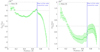 |
Fig. 1. Left panel: relative differences in squared adiabatic sound speed between the Sun and Seismic model 10 (Sismo 10). Right panel: relative differences in density between the Sun and Seismic Model 10 (Sismo 10). |
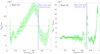 |
Fig. 2. Left panel: relative differences in entropy proxy, S5/3, between the Sun and Seismic Model 10 (Sismo 10). Right panel: differences in Ledoux discriminant between the Sun and Seismic Model 10 (Sismo 10). |
As we mentioned above, the reconstruction procedure does not explicitly apply corrections in A in the convective layers. This means that the corrections in these regions are solely a consequence of the modifications required to satisfy mass conservation in the reconstructed models. As we will see in Sect. 3.1 when looking at the changes in squared adiabatic sound speed at each iteration, the agreement in the convective envelope for this specific quantity is actually not improved over the reconstruction procedure. Consequently, it is clear that our seismic models do not provide as good an agreement in adiabatic sound speed in those regions as those determined in previous studies that explicitly corrected the profiles in the convective envelope (see e.g. Antia & Basu 1994b; Turck-Chièze et al. 2004; Vorontsov et al. 2014). This is a direct consequence of our reconstruction method, for which we chose to focus on the deeper radiative layers where the uncertainties on Γ1 are much smaller. Thus, in comparison to previous studies, our models perform very well in the deeper layers, especially for the density profile. This improvement of the density and entropy proxy profiles over the course of the iterations is a direct consequence of the mass conservation. Indeed, even if the convective layers are left untouched, the variations of density resulting from the A corrections applied in the radiative interior will be compensated by larger variations in the upper, less-dense, convective layers, leading to an improvement of the agreement with the Sun for both density and entropy proxy.
The corrections to the Ledoux discriminant were still applied at the exact location of the BCZ, using the δA amplitude given by the inversion point with the closest central value of the averaging kernels. In the cases considered here, this only implies a minimal shift, well within both the vertical and resolution error bars of the inversion.
We thus define a unique set of thermodynamical variables, ρ, P, and Γ1 at this location; these variables will define the properties of the lower convective envelope in hydrostatic equilibrium. However, since the radial position of the transition between convective and radiative regions determined from the Schwarzschild criterion was not modified in the reconstruction, the determined seismic model will not exactly follow the same density profiles in the convective envelope, as we will see later. In the deep convective layers, the behaviour of the seismic model will essentially be determined by the original A and Γ1 profiles as well as by the satisfaction of hydrostatic equilibrium through the determination of m(r) at a given radius.
Another region left untouched in the reconstruction procedure is the surface layers of the model, namely the substantially super-adiabatic convective layers as well as the atmosphere. This choice is justified by the fact that inversions based on the variational principle of adiabatic stellar oscillations are unable to provide reliable constraints in these regions; thus, the inferred corrections would not be appropriate. This also justifies the use of different atmosphere models and formalisms of convection, as we can then directly measure their impact on the final reconstructed structure of the Sun (see Sect. 4).
In the right-hand panel of Fig. 3, we illustrate the convergence of the reconstruction procedure for Model 10. The final agreement in Ledoux discriminant inversions for all models in our sample is illustrated in the left-hand panel of Fig. 3, and a selection of the corresponding Ledoux discriminant profiles are illustrated in Fig. 8. As can be seen, the agreement is excellent in the deep radiative layer, whatever the initial conditions. Small discrepancies can be seen just below the BCZ at the resolution limit of the SOLA inversion. The central regions (below 0.08 R⊙) are also slightly different, since they were not modified during the reconstruction procedure.
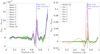 |
Fig. 3. Left panel: illustration of the agreement in Ledoux discriminant for the reconstructed models using the reference models of Table 1 as initial conditions. Right panel: illustration of the convergence of the A corrections for successive iterations of the reconstruction procedure in the case of Model 10. |
From the analysis of the Ledoux discriminant inversions, we can conclude that the reconstruction procedure was able to provide a precise, model-independent profile of this quantity in the Sun, which can be used to analyse the limitations of the current models. As mentioned previously, another key aspect for future advances in helioseismology is the potential observation of gravity modes. Below ≈200 μHz, the gravity modes follow a regular pattern and are described to the first order by an asymptotic expression as a function of their period, Pn, ℓ
 (5)
(5)
where n is the radial order, ℓ is the degree, υ is a phase shift depending on the properties near the BCZ and P0 is defined by
 (6)
(6)
where N the Brunt-Väisälä is frequency and rBCZ is the radial position of the BCZ. This implies that the separation between two modes of consecutive n in the asymptotic regime, defined as the asymptotic period spacing, is determined by P0 (i.e. by the integral of the Brunt-Väisälä frequency up to the BCZ).
We illustrate the results of these integrals of P0 for our seismic and reference models in Table 2, which shows that despite having good constraints on the Ledoux discriminant in the deep radiative layer of the Sun, the fact that we are missing the deep core still allows for a significant variation of the period spacing of g-modes in our sample of reconstructed structures. Typically, we find a range of period spacing values spanning an interval of 25 s, far from the observed value of 2040 s in Fossat et al. (2017) but closer to the theoretical value of 2105 s in Provost et al. (2000). Only slight changes in the period spacing values, of the order of 10 s, are found if the reconstruction procedure is carried out using GOLF data from Salabert et al. (2015) instead of BiSON data for the low-degree modes. However, these determined values can be changed significantly by altering the A profile below 0.08 R⊙ without destroying the agreement with the inversion results from p-modes. Hence, another input is required to better constrain the expected period spacing of the solar gravity modes. This will be further discussed in Sect. 4 when studying the impact of the choice of the reference model.
Comparison between period spacing values for the seismic models after seven iterations and the reference models values.
3. Agreement with other seismic indices
In the previous section, we focused on demonstrating that using successive inversions of the Ledoux discriminant allowed us to determine a model-independent profile for this quantity. However, the main benefit of the reconstruction procedure is that it allowed to determine fully consistent seismic models of the solar structure, which are also in excellent agreement in terms of other structural variables. In this section, we will show that once the reconstruction procedure has converged, we reach a level of agreement in the radiative zone of ≈0.1% for structural inversions of ρ, c2 and S5/3 = P/ρ5/3. This implies that most of the issues with our depiction of the solar structure are clearly related to the radiative layers, as we are able to efficiently suppress other traces of mismatches by correcting A in the radiative region.
3.1. Sound-speed inversions
The sound-speed inversions were carried out using the (c2, ρ) kernels in Eq. (3). As can be seen from the left-hand panel of Fig. 4, the agreement for all models is of ≈0.1% in the radiative region and the lower parts of the convective region. From the right-hand panel of Fig. 4, we also see that, as mentioned earlier, the sound-speed profile in the convective envelope was not corrected by the reconstruction procedure, as no corrections in A were applied in the convective envelope.
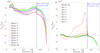 |
Fig. 4. Left panel: agreement in relative sound-speed differences for the reconstructed models using the reference models of Table 1 as initial conditions. Right panel: illustration of the convergence of the sound-speed relative differences for successive iterations of the reconstruction procedure in the case of Model 10. |
These results confirm that, as expected, the solar modelling problem is mostly an issue related to the temperature gradient of the low-metallicity models in the radiative regions. However, from the analysis of the successive changes due to the iterations in the reconstruction procedure, illustrated in the right-hand panel of Fig. 4, we can see that the bulk of the profile is corrected after the third reconstruction. The first step mostly corrects the sound-speed discrepancy in the radiative zone, near the BCZ. The remaining discrepancies are efficiently corrected in the following iterations. However, one can see that there is a remaining discrepancy, even for the model obtained after seven iteration. These variations remain very small and are not linked to significant deviations in the A profile. They do not seem to be linked to Γ1 differences between the models, but rather to the position of the BCZ and the mass coordinate at that position. Indeed, these parameters determine the density profile of the models and it is clear that the models with the worst agreement on the position of the BCZ with respect to the helioseismic value of 0.713 ± 0.001 R⊙ also have the largest discrepancies in both sound-speed and, as shown in Sect. 3.3, density profiles. This implies that an additional selection of the models based on their position of the BCZ and the mass coordinate at the BCZ could be used as a second step. Unfortunately, we do not have a direct measurement of the mass coordinate at the BCZ. Vorontsov et al. (2014) were able to determine the mass coordinate at 0.75 R⊙, m0.75 = 0.9822 ± 0.0002 M⊙ and discussed its importance as a calibrator of the specific entropy in the solar convective envelope. All our reconstructed models are in good agreement with the determined value of the m0.75 parameter in Vorontsov et al. (2014), as illustrated in Table 3. Similarly, they all show very good agreement in entropy proxy inversions, as we will further discuss in Sect. 3.2.
Comparison between m0.75 for the seismic models after seven iterations and their corresponding reference models values.
3.2. Entropy proxy inversions
The entropy proxy inversions were carried out using the (S5/3, Γ1) kernels in Eq. (3). These kernels were presented in Buldgen et al. (2017b) and applied to the solar case in Buldgen et al. (2017a, 2019). From the left-hand panel of Fig. 5, we can see that the agreement for this inversion is also of ≈0.1% in the radiative and convective regions for all models, whatever their initial conditions. This confirms that correcting for the A profile in the radiative region leads to an excellent agreement of the height of the plateau in the convective zone.
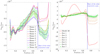 |
Fig. 5. Left panel: agreement in relative entropy proxy differences for the reconstructed models using the reference models of Table 1 as initial conditions. Right panel: illustration of the convergence of the entropy proxy relative differences for successive iterations of the reconstruction procedure in the case of Model 10. |
From a closer analysis of the reconstruction procedure, we can see that a good agreement of the height of the plateau is reached after three iterations. The explanation for this is found in the form of the applied corrections to the model. At first, the reconstruction procedure is dominated by the large discrepancies near the BCZ in all models. Once these differences are partially corrected, we can see in the right-hand panel of Fig. 5 that the corrections in the deeper layer of the radiative zone remain significant for the second iteration. It then takes two iterations to completely erase discrepancies in the A profile below 0.6 R⊙. Once this is achieved, the inferred A profile shows an oscillatory behaviour in these regions (as seen in Fig. 3). This phenomenon is linked to a form of the Gibbs phenomenon, due to the fact that the remaining deviations are located in a very narrow region, just below the BCZ, and are too sharp to be properly sampled by the classical SOLA method we use in this study. From a physical point of view, the remaining discrepancies may originate from multiple contributions, including a slight mismatch between the transition from the radiative to convective outward transport of energy, which causes a sharp variation in A and a mismatch in A in the last percent of solar radii just below the BCZ. Of course, it should be recalled that a breaking of spherical symmetry in the structure of the tachocline region could also lead to mismatches with any modelling that assumes spherical symmetry.
3.3. Density inversions
The density inversions were carried out using the (ρ, Γ1) structural kernels, ensuring that the total solar mass is conserved during the inversion procedure. By using the (ρ, Γ1) kernels, we ensured an intrinsically low contribution of the cross-term, as the relative variations of Γ1 were expected to be very small in most of the solar structure. The inversion results for all models are illustrated in the left-hand panel of Fig. 6. From these results, it appears that most of the models show an excellent agreement in density, of around 0.2% in the radiative layers. The closest models with respect to the Sun show an agreement below 0.1% throughout most of the solar structure, and the worst offenders show discrepancies as high as 0.25% in the deep layers. These are also the models showing the large discrepancies in sound speed discussed earlier, and thus the disagreements we find are actually due to the fact that these models do not fit well the position of the BCZ of 0.713 ± 0.001 R⊙. As discussed in Sect. 3.1, this means that a second selection can be performed based on the position of the BCZ. This aspect, however, does not have any implication regarding chemical abundances but solely constrains further the behaviour of the Ledoux discriminant around the BCZ and thus has strong implications on the properties of the macroscopic mixing in those layers. However, due to the lack of resolution in the inversion procedure, a definitive answer at the BCZ will likely need to come from non-linear inversions adapted to sample steep gradients of the function to be determined from the seismic data.
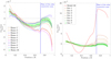 |
Fig. 6. Left panel: agreement in relative density differences for the reconstructed models using the reference models of Table 1 as initial conditions. Right panel: illustration of the convergence of the density relative differences for successive iterations of the reconstruction procedure in the case of Model 10. |
Taking a look at the right-hand panel of Fig. 6, we can see that the first reconstruction step leads to a significant improvement of the density profile. Unlike the sound-speed inversion, the second and third steps lead to smaller improvement in the inversion results in radiative layers. This is also seen in the entropy proxy inversion, where the leap after the first reconstruction step is mainly due to the corrections of the discrepancies around 0.6 R⊙; however, the better overall agreement in the radiative region is mainly due to finer corrections at higher temperatures. This is also consistent with the results of Buldgen et al. (2019), where a localized change of the mean Rosseland opacity could provide some improvement in sound speed and Ledoux discriminant, but was not enough to provide an excellent agreement regarding the entropy proxy inversion.
3.4. Frequency-separation ratios
As a last verification step of the reconstruction procedure, we take a look at the so-called frequency-separation ratios, defined in Roxburgh & Vorontsov (2003), of the six of our reconstructed solar models. These quantities are defined as the ratio of the so-called small frequency separation over the large frequency separation ratio as follows
 (7)
(7)
 (8)
(8)
with νℓ, n the frequency of radial order n and degree ℓ.
In Fig. 7, we plot the difference between the observed frequency-separation ratios and those of our seismic models, normalised by their 1σ uncertainties. As can be seen, the agreement for all models is excellent. From the comparison with the results of Model 1 in blue, we can see that the improvement in the agreement is quite significant. This is no surprise, as the reconstruction is based on reproducing the Ledoux discriminant inversions, which are closely linked to the sound-speed gradient and thus to the frequency-separation ratios, following the asymptotic developments from Shibahashi (1979) and Tassoul (1980). This also means that the frequency-separation ratios, like any other classic helioseismic investigation (e.g. structural inversions), are by no means a direct measurement of the chemical abundances in the deep radiative layers. As a consequence, they cannot be employed to advocate the use of any particular abundance table for the construction of solar models.
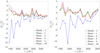 |
Fig. 7. Agreement in frequency-separation ratios of low-degree p-modes for six reconstructed models using the corresponding references of Table 1 as initial conditions, as well as reference Model 1 shown as comparison. |
4. Impact of reference models
While the reconstruction procedure leads to a very similar Ledoux discriminant profile for a wide range of initial model properties, it might not be fully justified to say that it is completely independent of the initial conditions of the procedure. In the previous sections, we discussed how the position of the BCZ could affect the final agreement for sound-speed, density, and entropy proxy inversions.
However, this impact can be easily measured from the combination of multiple structural inversions and lead, to some extent, to an additional selection of the optimal seismic structure of the Sun. Other effects, such as the selected dataset or the assumed behaviour of the surface correction may lead to slight differences at the level of agreement we seek with such a reconstruction procedure. Using, for example, an extended MDI dataset such as the one in Reiter et al. (2015, 2020) may provide ways to further test the robustness of our procedure, as well as better probe the agreement of our seismic model of the Sun in the convective envelope. Indeed, from the comparison of models Sismo 1, Sismo 8, and Sismo 9, we can see that some small variations in the upper envelope properties remain after the reconstruction procedure. The changes in the radiative region between these models are, unsurprisingly, much smaller. This implies that additional insight can be gained from using an extended dataset probing the upper convective layers in a more stringent manner, as in Di Mauro et al. (2002) and Vorontsov et al. (2013).
The approach used to connect the regions on which the A corrections are applied to the central regions may also locally impact the procedure. Obviously, the fact that no corrections are applied below 0.08 R⊙ leaves a direct mark on the final reconstructed structure. This is illustrated in Figs. 8 and 9, where we plot the Ledoux discriminant, Brunt-Väisälä frequency and sound-speed profiles of all our reconstructed models in the deep solar core. From the inspection of the right-hand panel of Fig. 8, we can better understand the behaviour of the period spacing changes of Table 2. Indeed, Models 1 and 7 show some minor changes in asymptotic period spacing, while the spacing of Model 5 is significantly corrected. This is simply due to the fact that Models 1 and 7 reproduce the Brunt-Väisälä frequency of the Sun in the deep radiative layers much better. However, as we lack constraints below 0.08 R⊙, we cannot state with full confidence that the observed period spacing will lie within the 25 s range we find.
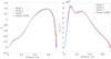 |
Fig. 8. Left panel: Ledoux discriminant profiles from the reconstruction procedure. The dashed lines illustrate the reference profile of some of the models in Table 1 while the continuous lines show the profile on which the procedure converges (using all reference models). Right panel: same as the left panel but for the Brunt-Väisälä frequency. |
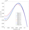 |
Fig. 9. Sound-speed profile in the core region of the reconstructed model, showing the impact of initial conditions in the deep solar core, that is unconstrained by p-modes. |
The optimal approach to lifting the degeneracy in the inner core would be to have an observed value of the period spacing of the solar gravity modes at our disposal. Including constraints from neutrino fluxes may already provide additional constraints. However, their main limitation is that, in this case, we would have to assume a given composition profile for our solar models, a given equation of state, and nuclear reaction rates. Taking these constraints into account implies that we use all our current knowledge regarding the present day solar structure. However, this would be at the expense of adding more uncertainties and “model-dependencies” into the procedure. In their paper, Shibahashi & Takata (1996) only made an assumption regarding Z(r), the distribution of heavy elements in the solar interior, but they solved the equation of radiative transfer and thus assumed the mean Rosseland opacity to be known. Given the current uncertainties on radiative opacities, it might be safer to avoid such an assumption, especially at lower temperatures.
Unravelling the core properties of the Sun would be crucial for the theory of stellar physics. First, it would allow us to constrain the angular momentum transport processes acting in solar and stellar radiative zones, as discussed in Eggenberger et al. (2019). Second, it would demonstrate whether the solar core has undergone intermittent mixing, for example due to out-of-equilibrium burning of 3He (Dilke & Gough 1972; Unno 1975; Gabriel et al. 1976) or a prolonged lifetime of its transitory convective core in the early main-sequence evolution. Third, it would also allow us to constrain nuclear reaction rates and their screening factors, as these remain key ingredients of stellar models that are quite uncertain from a theoretical point of view (see e.g. Mussack & Däppen 2011; Mussack 2011, for a discussion).
5. Limitations and uncertainties
In the previous sections, we demonstrated how the inversion of the Ledoux discriminant can be used to build a seismic Sun from successive correction, integration and inversion steps. While the process is quite straightforward and allows us to test the consistency between different inversions of the solar structure, it also suffers from intrinsic limitations.
The first limitation is due to the incomplete information given by the inversion technique. Indeed, since p-modes do not allow us to test solar models below 0.08 R⊙, we are not able to get a full view of the seismic Sun. While this region only represents 8% of the solar structure in radial extent, it also represents ≈3% in mass of the solar structure, which actually corresponds to the total mass of the solar convective envelope. This implies that an accurate depiction of the mass distribution inside the Sun can only obtained if we observe solar g-modes. This is also illustrated in the results of Table 2, which shows that the reconstruction only slightly alters the values of the period spacing. Obtaining a precise measurement of that quantity would indeed provide a strong additional selection to the set of seismic models and allow for joint analyses using both neutrino flux measurement and helioseismology.
The second main limitation also stems from the inversion procedure and is linked to the impact of the surface effects. Indeed, as can be seen from sound-speed, entropy proxy and density inversions, the upper layer of the model was not extensively probed by the inversion procedure. Since we only applied corrections to A in the internal radiative layers, this does not render the reconstruction procedure meaningless. However, this means that the conclusions we can draw from the other inversion procedures used as sanity checks are mostly limited to the lower parts of the envelope and the radiative region. This implies that to better constrain the properties of the solar convective envelope (composition, equation of state, etc), we will have to extend the dataset to higher degree modes. Of course, this means that we will have to be more attentive to the surface effects that can lead to biases in the determined corrections from these higher frequency modes (see e.g. Gough & Vorontsov 1995).
Not applying the corrections in the convective envelope is also a clear limiting factor of our method. While the improvement is significant when comparing the initial models in terms of density and entropy proxy profile, it is also clear that the sound -speed profile in the convective envelope is not extensively corrected by our method. This leads our seismic models to be somewhat less performant in terms of sound speed in the convective envelope, while being more performant in the radiative region, especially regarding density and entropy proxy inversions. Consequently, a promising way of obtaining a very accurate picture of the internal structure of the Sun from helioseismology would be to combine our reconstruction technique with those focusing on obtaining optimal models of the solar convective envelope (as shown for example in Vorontsov et al. 2014).
In addition to these limitations, which are intrinsic to the use of seismic inversions from solar acoustic oscillations, we have also made the hypothesis to keep the Γ1 profile and the position of the BCZ unchanged in the reconstruction procedure. The BCZ position is not a strong limitation, as it can easily be avoided by ensuring that the reference model agrees with the helioseismically determined value. As we saw in Fig. 8, this has no impact on the final Ledoux discriminant profile determined by the reconstruction procedure.
The hypothesis of unchanged Γ1 can be more severe if we start looking at changes in the thermodynamical quantities of small amplitude. Indeed, Vorontsov et al. (2014) reported measurements of the  profile of a precision of up to 10−4 in the deepest half of the convection zone, which is just one order of magnitude bigger than the estimated precision of equation of state interpolation routines (Baturin et al. 2019). This implies that, at the magnitude of the relative differences we see in the solar convective envelope, keeping Γ1 constant might not be a good strategy; it also implies that we have to become attentive to the intrinsic numerical limitations of the tabulated ingredients of our solar models.
Moreover, intrinsic changes between different equations of state will necessarily lead to slight differences in the determined profiles. Since the Γ1 profile in the convective envelope is strongly tied to the assumed chemical composition of the envelope, this also means that the envelope properties of our seismic models may not be fully consistent. Indeed, the density, pressure, and Γ1 profiles are determined (or fixed) in our approach. Providing consistent profiles of X, Z and T for the reconstructed structure might very likely require us to assume changes in Γ1 in the envelope of our models. This is beyond the scope of this study but will be addressed in the future using the most recent versions of equations of state available (Baturin et al. 2013) and using Γ1 inversions in the solar envelope.
In the radiative layers, the hypothesis of unchanged Γ1 is less constraining, as one can safely assume that the A corrections will be largely dominated by the contributions from the pressure and density gradients. However, there is still a degeneracy between temperature and chemical composition, which can lead to changes in both pressure and density profiles, even if an equation of state is assumed. This is also a clear limitation of our procedure, but it is intrinsic to its seismic nature.
A third limitation of our reconstruction is also linked to the seismic data used. We carried out additional tests using MDI data from Larson & Schou (2015) and from the latest release following the fitting methodology of Korzennik (2005); Korzennik (2008a), and Korzennik (2008b) for the medium- and high-degree modes combined with GOLF data instead of BiSON data for low-degree modes and saw that variations of up to ≈3 × 10⁻³ could be found in the sound-speed profiles of the seismic models; on the other hand, using the latest MDI datasets with the BiSON data led to changes of about ≈1 × 10⁻³, and using GOLF data from (Salabert et al. 2015) instead of BiSON data with the original MDI dataset led to similar deviations. The largest differences, however, were found below 0.08 R⊙, in a region uncontrolled by the reconstruction procedure. This implies that the actual accuracy of the reconstruction is tightly linked to the dataset used.
6. Conclusion
We have presented a new approach to computing a seismic Sun, taking advantage of the Ledoux discriminant inversions to limit the amount of numerical differentiations when computing the solar structure. Our approach allows us to provide a full profile of the Ledoux discriminant for our seismic models. To verify the consistency and robustness of our method, we checked that it also led to an improvement of other classical helioseismic indicators such as frequency-separation ratios, as well as other structural inversions. By selecting models with the exact position of the discontinuity in A determined by helioseismology, the reconstructed models agree with the Sun well within 0.1% for all other structural inversions in the radiative interior. Slightly larger differences can be seen depending on the dataset used to carry out the reconstruction.
Our procedure converges consistently on a unique estimate of the solar Ledoux discriminant within the range of radii on which the inversions are considered reliable. This approach opens up new ways of analysing the current uncertainties on the solar temperature gradient, as the main advantage of the Ledoux discriminant is that it is largely dominated by the contribution of the difference between the temperature gradient and the adiabatic temperature gradient in most of the radiative zone. This also opens up the possibility of directly estimating the expected opacity modification for a given equation of state and a given chemical composition, providing key insights to the opacity community (see also Gough 1976). This approach provides a complementary way to estimate the required modifications expected to be a key element in solving the current stalemate regarding solar abundances following their revision by Asplund et al. (2009).
In the regions where the mean molecular weight term of A has a non-negligible contribution (close to the BCZ and in regions affected by nuclear reactions), further degeneracies, and thus larger uncertainties, can be expected. However, by analysing these effects, we can expect to gain insights into the properties of microscopic diffusion and mixing at the BCZ. Gaining more insights into the behaviour of the discontinuity in the A profile in the tachocline region will require using one of our seismic models as a reference for non-linear RLS inversions as in Corbard et al. (1999), allowing for solutions of the inversion displaying larger gradients. This will be done in future studies.
In the convective envelope, the reconstruction procedure allows us to set a good basis for precise determinations of the composition in this region, especially for Z, improving on Buldgen et al. (2017d) and tests of the equation of state used in solar and stellar models. Indeed, this requires that contaminations from the unavoidable cross-term contributions of the inversion are limited as much as possible while still allowing for the testing of different equations of states. By using higher ℓ modes (Reiter et al. 2015, 2020), we can expect to further test the robustness of our approach in the convective envelope and provide estimates of the physical properties of the Sun in this region.
Gaining more information on the solar core will very likely be more difficult, as the procedure is intrinsically limited by the solar p-modes. However, combining it with neutrino fluxes may provide a way to further constrain the solar structure. In addition, it may also be useful to predict the expected range of the asymptotic value of the period spacing of g-modes, helping with their detection. This is particularly timely, given the recent discussions in the literature about the potential detection of these modes (Fossat et al. 2017; Fossat & Schmider 2018; Schunker et al. 2018; Appourchaux & Corbard 2019; Scherrer & Gough 2019) and the renewed interest it inspired in the quest to find them. Should this additional seismic constraint become available, it could easily be included in the procedure and usher in a new era of solar physics. As such, the Sun still remains an excellent laboratory for fundamental physics and the current study provides a new, original way to exploit the information available from the observation of acoustic oscillations.
We note that similar data are given in Gough (1976), page 14, but these data were unfortunately provided before the revision of the abundances and the subsequent appearance of the so-called “solar modelling problem”.
This is the region marking the transition between the latitudinal differential rotation in the solar convection envelope and the rigid rotation of the radiative interior and may be subject to extra mixing.
Additional descriptions of similar numerical procedures are available in Scuflaire et al. (2008b).
Acknowledgments
We thank the referee for the useful comments that have substantially helped to improve the manuscript. G.B. acknowledges fundings from the SNF AMBIZIONE grant No 185805 (Seismic inversions and modelling of transport processes in stars). P.E. and S. J. A. J. S. have received funding from the European Research Council (ERC) under the European Union’s Horizon 2020 research and innovation programme (grant agreement No 833925, project STAREX). This article used an adapted version of InversionKit, a software developed within the HELAS and SPACEINN networks, funded by the European Commissions’s Sixth and Seventh Framework Programmes. Funding for the Stellar Astrophysics Centre is provided by The Danish National Research Foundation (Grant DNRF106). We acknowledge support by the ISSI team “Probing the core of the Sun and the stars” (ID 423) led by Thierry Appourchaux.
References
- Adelberger, E. G., García, A., Robertson, R. G. H., et al. 2011, Rev. Mod. Phys., 83, 195 [NASA ADS] [CrossRef] [Google Scholar]
- Antia, H. M., & Basu, S. 1994a, ApJ, 426, 801 [NASA ADS] [CrossRef] [Google Scholar]
- Antia, H. M., & Basu, S. 1994b, A&AS, 107, 421 [NASA ADS] [Google Scholar]
- Antia, H. M., & Basu, S. 2005, ApJ, 620, L129 [NASA ADS] [CrossRef] [Google Scholar]
- Appourchaux, T., & Corbard, T. 2019, A&A, 624, A106 [NASA ADS] [CrossRef] [EDP Sciences] [Google Scholar]
- Asplund, M., Grevesse, N., Sauval, A. J., & Scott, P. 2009, ARA&A, 47, 481 [NASA ADS] [CrossRef] [Google Scholar]
- Ayukov, S. V., & Baturin, V. A. 2011, J. Phys. Conf. Ser., 271, 012033 [NASA ADS] [CrossRef] [Google Scholar]
- Ayukov, S. V., & Baturin, V. A. 2017, Astron. Rep., 61, 901 [CrossRef] [Google Scholar]
- Bailey, J. E., Nagayama, T., Loisel, G. P., et al. 2015, Nature, 517, 3 [Google Scholar]
- Basu, S., & Antia, H. M. 1995, MNRAS, 276, 1402 [NASA ADS] [Google Scholar]
- Basu, S., & Antia, H. M. 1997, MNRAS, 287, 189 [NASA ADS] [CrossRef] [Google Scholar]
- Basu, S., & Antia, H. M. 2008, Phys. Rep., 457, 217 [NASA ADS] [CrossRef] [Google Scholar]
- Basu, S., & Thompson, M. J. 1996, A&A, 305, 631 [Google Scholar]
- Basu, S., Chaplin, W. J., Elsworth, Y., New, R., & Serenelli, A. M. 2009, ApJ, 699, 1403 [NASA ADS] [CrossRef] [Google Scholar]
- Baturin, V. A., Ayukov, S. V., Gryaznov, V. K., et al. 2013, in Progress in Physics of the Sun and Stars: A New Era in Helio- and Asteroseismology, eds. H. Shibahashi, A. E. Lynas-Gray, et al., ASP Conf. Ser., 479, 11 [Google Scholar]
- Baturin, V. A., Däppen, W., Oreshina, A. V., Ayukov, S. V., & Gorshkov, A. B. 2019, A&A, 626, A108 [CrossRef] [EDP Sciences] [Google Scholar]
- Benomar, O., Takata, M., Shibahashi, H., Ceillier, T., & García, R. A. 2015, MNRAS, 452, 2654 [NASA ADS] [CrossRef] [Google Scholar]
- Bergemann, M., & Serenelli, A. 2014, in Solar Abundance Problem, in Determination of Atmospheric Parameters of B-, A-, F- and G-Type Stars: Lectures from the School of Spectroscopic Data Analyses, eds. E. Niemczura, B. Smalley, & W. Pych (Cham: Springer International Publishing), 245 [Google Scholar]
- Blancard, C., Colgan, J., Cossé, P., et al. 2016, Phys. Rev. Lett., 117, 249501 [NASA ADS] [CrossRef] [Google Scholar]
- Brown, T. M., & Morrow, C. A. 1987, in The Internal Solar Angular Velocity, eds. B. R. Durney, & S. Sofia, Astrophys. Space Sci. Libr., 137, 7 [NASA ADS] [CrossRef] [EDP Sciences] [Google Scholar]
- Buldgen, G., Salmon, S. J. A. J., Noels, A., et al. 2017a, A&A, 607, A58 [NASA ADS] [CrossRef] [EDP Sciences] [Google Scholar]
- Buldgen, G., Reese, D. R., & Dupret, M. A. 2017b, A&A, 598, A21 [NASA ADS] [CrossRef] [EDP Sciences] [Google Scholar]
- Buldgen, G., Salmon, S. J. A. J., Godart, M., et al. 2017c, MNRAS, 472, L70 [NASA ADS] [CrossRef] [Google Scholar]
- Buldgen, G., Salmon, S. J. A. J., Noels, A., et al. 2017d, MNRAS, 472, 751 [CrossRef] [Google Scholar]
- Buldgen, G., Salmon, S. J. A. J., Noels, A., et al. 2019, ArXiv e-prints [arXiv:1902.10390] [Google Scholar]
- Canuto, V. M., & Mazzitelli, I. 1991, ApJ, 370, 295 [NASA ADS] [CrossRef] [Google Scholar]
- Canuto, V. M., & Mazzitelli, I. 1992, ApJ, 389, 724 [NASA ADS] [CrossRef] [Google Scholar]
- Canuto, V. M., Goldman, I., & Mazzitelli, I. 1996, ApJ, 473, 550 [NASA ADS] [CrossRef] [Google Scholar]
- Charbonnel, C., & Talon, S. 2005, Science, 309, 2189 [Google Scholar]
- Christensen-Dalsgaard, J., & Houdek, G. 2010, Ap&SS, 328, 51 [NASA ADS] [CrossRef] [Google Scholar]
- Christensen-Dalsgaard, J., Duvall, T. L. J., Gough, D. O., Harvey, J. W., & Rhodes, E. J. J. 1985, Nature, 315, 378 [NASA ADS] [CrossRef] [Google Scholar]
- Christensen-Dalsgaard, J., Thompson, M. J., & Gough, D. O. 1989, MNRAS, 238, 481 [NASA ADS] [CrossRef] [Google Scholar]
- Christensen-Dalsgaard, J., Gough, D. O., & Thompson, M. J. 1991, ApJ, 378, 413 [NASA ADS] [CrossRef] [Google Scholar]
- Christensen-Dalsgaard, J., Gough, D. O., & Knudstrup, E. 2018, MNRAS, 477, 3845 [NASA ADS] [CrossRef] [Google Scholar]
- Colgan, J., Kilcrease, D. P., Magee, N. H., et al. 2016, ApJ, 817, 116 [NASA ADS] [CrossRef] [Google Scholar]
- Corbard, T., Blanc-Féraud, L., Berthomieu, G., & Provost, J. 1999, A&A, 344, 696 [NASA ADS] [Google Scholar]
- Cox, J., & Giuli, R. 1968, Principles of Stellar Structure: Applications to stars (Gordon and Breach) [Google Scholar]
- Davies, G. R., Broomhall, A. M., Chaplin, W. J., Elsworth, Y., & Hale, S. J. 2014, MNRAS, 439, 2025 [Google Scholar]
- Deheuvels, S., García, R. A., Chaplin, W. J., et al. 2012, ApJ, 756, 19 [NASA ADS] [CrossRef] [Google Scholar]
- Deheuvels, S., Doğan, G., Goupil, M. J., et al. 2014, A&A, 564, A27 [NASA ADS] [CrossRef] [EDP Sciences] [Google Scholar]
- Dilke, F. W. W., & Gough, D. O. 1972, Nature, 240, 262 [NASA ADS] [CrossRef] [Google Scholar]
- Di Mauro, M. P., Christensen-Dalsgaard, J., Rabello-Soares, M. C., & Basu, S. 2002, A&A, 384, 666 [NASA ADS] [CrossRef] [EDP Sciences] [Google Scholar]
- Dziembowski, W. A., Pamyatnykh, A. A., & Sienkiewicz, R. 1990, MNRAS, 244, 542 [NASA ADS] [Google Scholar]
- Dziembowski, W. A., Pamiatnykh, A. A., & Sienkiewicz, R. 1991, MNRAS, 249, 602 [NASA ADS] [CrossRef] [Google Scholar]
- Eggenberger, P., Maeder, A., & Meynet, G. 2005, A&A, 440, L9 [NASA ADS] [CrossRef] [EDP Sciences] [Google Scholar]
- Eggenberger, P., Buldgen, G., & Salmon, S. J. A. J. 2019, A&A, 626, L1 [NASA ADS] [CrossRef] [EDP Sciences] [Google Scholar]
- Elliott, J. R. 1996, MNRAS, 280, 1244 [NASA ADS] [CrossRef] [Google Scholar]
- Ferguson, J. W., Alexander, D. R., Allard, F., et al. 2005, ApJ, 623, 585 [NASA ADS] [CrossRef] [Google Scholar]
- Fossat, E., & Schmider, F. X. 2018, A&A, 612, L1 [NASA ADS] [CrossRef] [EDP Sciences] [Google Scholar]
- Fossat, E., Boumier, P., Corbard, T., et al. 2017, A&A, 604, A40 [NASA ADS] [CrossRef] [EDP Sciences] [Google Scholar]
- Gabriel, M., Noels, A., Scuflaire, R., & Boury, A. 1976, A&A, 47, 137 [Google Scholar]
- Gough, D. 1976, in Equation-of-State and Phase-Transition in Models of Ordinary Astrophysical Matter, eds. V. Celebonovic, D. Gough, & W. Däppen, Am. Inst. Phys. Conf. Ser., 731, 119 [Google Scholar]
- Gough, D. O., & Kosovichev, A. G. 1993, MNRAS, 264, 522 [NASA ADS] [CrossRef] [Google Scholar]
- Gough, D. O., & McIntyre, M. E. 1998, Nature, 394, 755 [NASA ADS] [CrossRef] [Google Scholar]
- Gough, D. O., & Scherrer, P. H. 2001, in The solar interior, in The Century of Space Science, eds. J. A. M. Bleeker, J. Geiss, & M. C. E. Huber (Dordrecht: Springer, Netherlands), 1035 [CrossRef] [Google Scholar]
- Gough, D. O., & Vorontsov, S. V. 1995, MNRAS, 273, 573 [NASA ADS] [CrossRef] [Google Scholar]
- Grevesse, N., & Noels, A. 1993, in Origin and Evolution of the Elements, eds. N. Prantzos, E. Vangioni-Flam, & M. Casse, 15 [Google Scholar]
- Gryaznov, V. K., Ayukov, S. V., Baturin, V. A., et al. 2004, in Equation-of-State and Phase-Transition in Models of Ordinary Astrophysical Matter, eds. V. Celebonovic, D. Gough, W. Däppen, et al., Am. Inst. Phys. Conf. Ser., 731, 147 [NASA ADS] [CrossRef] [Google Scholar]
- Gryaznov, V. K., Ayukov, S. V., Baturin, V. A., et al. 2006, J. Phys. A: Math. General, 39, 4459 [NASA ADS] [CrossRef] [Google Scholar]
- Gryaznov, V., Iosilevskiy, I., Fortov, V., et al. 2013, Contrib. Plasma Phys., 53, 392 [NASA ADS] [CrossRef] [Google Scholar]
- Guzik, J. A., & Mussack, K. 2010, ApJ, 713, 1108 [NASA ADS] [CrossRef] [Google Scholar]
- Guzik, J. A., Watson, L. S., & Cox, A. N. 2006, Mem Soc. Astron. Italiana, 77, 389 [NASA ADS] [Google Scholar]
- Howe, R. 2009, Liv. Rev. Sol. Phys., 6, 1 [Google Scholar]
- Iglesias, C. A. 2015, MNRAS, 450, 2 [NASA ADS] [CrossRef] [Google Scholar]
- Iglesias, C. A., & Hansen, S. B. 2017, ApJ, 835, 284 [NASA ADS] [CrossRef] [Google Scholar]
- Iglesias, C. A., & Rogers, F. J. 1996, ApJ, 464, 943 [NASA ADS] [CrossRef] [Google Scholar]
- Irwin, A. W. 2012, Astrophysics Source Code Library [record ascl:1211.002] [Google Scholar]
- Korzennik, S. G. 2005, ApJ, 626, 585 [NASA ADS] [CrossRef] [Google Scholar]
- Korzennik, S. G. 2008a, Astron. Nachr., 329, 453 [NASA ADS] [CrossRef] [Google Scholar]
- Korzennik, S. G. 2008b, J. Phys. Conf. Ser., 118, 012082 [NASA ADS] [CrossRef] [Google Scholar]
- Kosovichev, A. G. 1993, MNRAS, 265, 1053 [NASA ADS] [CrossRef] [Google Scholar]
- Kosovichev, A. G. 1999, J. Comput. Appl. Math., 109, 1 [NASA ADS] [CrossRef] [Google Scholar]
- Kosovichev, A. G. 2011, Advances in Global and Local Helioseismology: An Introductory Review, eds. J.-P. Rozelot, & C. Neiner (Berlin: Springer Verlag), Lecture Notes Phys., 832, 3 [Google Scholar]
- Kosovichev, A. G., & Fedorova, A. V. 1991, Soviet Ast., 35, 507 [NASA ADS] [Google Scholar]
- Krishna Swamy, K. S. 1966, ApJ, 145, 174 [NASA ADS] [CrossRef] [Google Scholar]
- Landi, E., & Testa, P. 2015, ApJ, 800, 110 [NASA ADS] [CrossRef] [Google Scholar]
- Larson, T. P., & Schou, J. 2015, Sol. Phys., 290, 3221 [NASA ADS] [CrossRef] [Google Scholar]
- Lund, M. N., Miesch, M. S., & Christensen-Dalsgaard, J. 2014, ApJ, 790, 121 [NASA ADS] [CrossRef] [Google Scholar]
- Marchenkov, K., Roxburgh, I., & Vorontsov, S. 2000, MNRAS, 312, 39 [NASA ADS] [CrossRef] [Google Scholar]
- Mondet, G., Blancard, C., Cossé, P., & Faussurier, G. 2015, ApJs, 220, 2 [NASA ADS] [CrossRef] [Google Scholar]
- Montalban, J., Miglio, A., Theado, S., Noels, A., & Grevesse, N. 2006, Commun. Asteroseismol., 147, 80 [NASA ADS] [CrossRef] [Google Scholar]
- Mosser, B., Goupil, M. J., Belkacem, K., et al. 2012, A&A, 548, A10 [NASA ADS] [CrossRef] [EDP Sciences] [Google Scholar]
- Mussack, K. 2011, Ap&SS, 336, 111 [CrossRef] [Google Scholar]
- Mussack, K., & Däppen, W. 2011, ApJ, 729, 96 [NASA ADS] [CrossRef] [Google Scholar]
- Nagayama, T., Bailey, J. E., Loisel, G. P., et al. 2019, Phys. Rev. Lett., 122, 235001 [Google Scholar]
- Nahar, S. N., & Pradhan, A. K. 2016, Phys. Rev. Lett., 116, 235003 [Google Scholar]
- Nielsen, M. B., Schunker, H., Gizon, L., Schou, J., & Ball, W. H. 2017, A&A, 603, A6 [NASA ADS] [CrossRef] [EDP Sciences] [Google Scholar]
- Pain, J. C., & Gilleron, F. 2019, https://doi.org/10.5281/zenodo.1590773 [Google Scholar]
- Pain, J.-C., & Gilleron, F. 2020, High Energy Density Phys., 34, 100745 [NASA ADS] [CrossRef] [Google Scholar]
- Pain, J. C., Gilleron, F., & Comet, M. 2018, in Workshop on Astrophysical Opacities, ASP Conf. Ser., 515, 35 [NASA ADS] [Google Scholar]
- Paquette, C., Pelletier, C., Fontaine, G., & Michaud, G. 1986, ApJS, 61, 177 [NASA ADS] [CrossRef] [Google Scholar]
- Pijpers, F. P., & Thompson, M. J. 1994, A&A, 281, 231 [NASA ADS] [Google Scholar]
- Pradhan, A. K., & Nahar, S. N. 2018, in Workshop on Astrophysical Opacities, ASP Conf. Ser., 515, 79 [NASA ADS] [Google Scholar]
- Provost, J., Berthomieu, G., & Morel, P. 2000, A&A, 353, 775 [NASA ADS] [Google Scholar]
- Prša, A., Harmanec, P., Torres, G., et al. 2016, AJ, 152, 41 [NASA ADS] [CrossRef] [Google Scholar]
- Rabello-Soares, M. C., Basu, S., & Christensen-Dalsgaard, J. 1999, MNRAS, 309, 35 [NASA ADS] [CrossRef] [Google Scholar]
- Reiter, J., Rhodes, E. J., Jr, Kosovichev, A. G., et al. 2015, ApJ, 803, 92 [NASA ADS] [CrossRef] [Google Scholar]
- Reiter, J., Rhodes, E. J. J., Kosovichev, A. G., et al. 2020, ApJ, 894, 80 [NASA ADS] [CrossRef] [Google Scholar]
- Richard, O., Dziembowski, W. A., Sienkiewicz, R., & Goode, P. R. 1998, A&A, 338, 756 [NASA ADS] [Google Scholar]
- Roxburgh, I. W., & Vorontsov, S. V. 2003, A&A, 411, 215 [NASA ADS] [CrossRef] [EDP Sciences] [Google Scholar]
- Salabert, D., García, R. A., & Turck-Chièze, S. 2015, A&A, 578, A137 [NASA ADS] [CrossRef] [EDP Sciences] [Google Scholar]
- Scherrer, P. H., & Gough, D. O. 2019, ApJ, 877, 42 [NASA ADS] [CrossRef] [Google Scholar]
- Schunker, H., Schou, J., Gaulme, P., & Gizon, L. 2018, Sol. Phys., 293, 95 [NASA ADS] [CrossRef] [Google Scholar]
- Scuflaire, R., Théado, S., Montalbán, J., et al. 2008a, Ap&SS, 316, 83 [Google Scholar]
- Scuflaire, R., Montalbán, J., Théado, S., et al. 2008b, Ap&SS, 316, 149 [Google Scholar]
- Serenelli, A. M., Basu, S., Ferguson, J. W., & Asplund, M. 2009, ApJ, 705, L123 [NASA ADS] [CrossRef] [Google Scholar]
- Shibahashi, H. 1979, PASJ, 31, 87 [NASA ADS] [Google Scholar]
- Shibahashi, H., & Takata, M. 1996, PASJ, 48, 377 [NASA ADS] [CrossRef] [Google Scholar]
- Shibahashi, H., Takata, M., & Tanuma, S. 1995, in Helioseismology, ESA Spec. Publ., 376, 9 [NASA ADS] [Google Scholar]
- Spada, F., Lanzafame, A. C., & Lanza, A. F. 2010, Ap&SS, 328, 279 [NASA ADS] [CrossRef] [Google Scholar]
- Spiegel, E. A., & Zahn, J. P. 1992, A&A, 265, 106 [NASA ADS] [Google Scholar]
- Spruit, H. C. 1999, A&A, 349, 189 [NASA ADS] [Google Scholar]
- Tassoul, M. 1980, ApJS, 43, 469 [NASA ADS] [CrossRef] [Google Scholar]
- Thompson, M. J., Toomre, J., Anderson, E. R., et al. 1996, Science, 272, 1300 [NASA ADS] [CrossRef] [PubMed] [Google Scholar]
- Thoul, A. A., Bahcall, J. N., & Loeb, A. 1994, ApJ, 421, 828 [NASA ADS] [CrossRef] [Google Scholar]
- Tikhonov, A. N. 1963, Soviet Math. Dokl., 4, 1035 [Google Scholar]
- Turck-Chièze, S., Couvidat, S., Piau, L., et al. 2004, Phys. Rev. Lett., 93, 211102 [NASA ADS] [CrossRef] [PubMed] [Google Scholar]
- Unno, W. 1975, PASJ, 27, 81 [NASA ADS] [Google Scholar]
- Vernazza, J. E., Avrett, E. H., & Loeser, R. 1981, ApJS, 45, 635 [Google Scholar]
- Vorontsov, S. V., Baturin, V. A., & Pamiatnykh, A. A. 1991, Nature, 349, 49 [NASA ADS] [CrossRef] [Google Scholar]
- Vorontsov, S. V., Baturin, V. A., Ayukov, S. V., & Gryaznov, V. K. 2013, MNRAS, 430, 1636 [NASA ADS] [CrossRef] [Google Scholar]
- Vorontsov, S. V., Baturin, V. A., Ayukov, S. V., & Gryaznov, V. K. 2014, MNRAS, 441, 3296 [NASA ADS] [CrossRef] [Google Scholar]
- Young, P. R. 2018, ApJ, 855, 15 [NASA ADS] [CrossRef] [EDP Sciences] [Google Scholar]
- Zaatri, A., Provost, J., Berthomieu, G., Morel, P., & Corbard, T. 2007, A&A, 469, 1145 [NASA ADS] [CrossRef] [EDP Sciences] [Google Scholar]
- Zhang, Q. S. 2014, ApJ, 787, L28 [NASA ADS] [CrossRef] [Google Scholar]
- Zhao, L., Eissner, W., Nahar, S. N., & Pradhan, A. K. 2018, in Workshop on Astrophysical Opacities, ASP Conf. Ser., 515, 89 [Google Scholar]
Appendix A: Numerical details of the reconstruction technique
As mentioned in Sect. 2, there are a few technical details related to the reconstruction procedure. Here, we briefly describe some of the numerical aspects used for this study3.
The reference models are evolutionary models computed using CLES. They typically contain between 1600 and 2500 layers, depending on the specifities input when running the evolutionary sequence. A typical evolutionary sequence for our reference models counts between 250 and 350 timesteps. The calibration on the solar parameters was carried out using a Levenberg-Marquardt algorithm, fitting the solar radius, the solar luminosity, and the current surface chemical composition at a level of 10−5 in relative error.
The reconstruction itself started with a local cubic spline interpolation in r2 using a Hermite polynomial defined by the function value and its derivative at each mesh interval. The derivatives were computed at each point from the analytical formulas of the second order polynomial associated with the interpolation. This interpolation of the reference model was carried out on a finer grid of typically 4000 to 5000 layers (although 3000 points might be sufficient if one wishes to compute g modes, as long as the sampling is good enough in the central regions). This step was made to ensure that the reintegration is done on a fine enough mesh after the corrections. The new grid points were added based on the variations of r, m1/3, log P, log ρ and Γ1.
The A profile resulting from the inversion was then interpolated on this grid between 0.08 R⊙ and the BCZ of the model. No corrections were applied above the BCZ of the model. Below 0.08 R⊙, the fact that we do not add the A corrections will lead to an unphysical discontinuity. To avoid this, we reconnected the corrected and the uncorrected profiles by interpolating them on ≈20 layers. This means that the A profile below 0.08 R⊙ will remain that of the reference model. An example of such a reconnection is shown in Fig. A.1 As described in Sect. 2, the Γ1 profile was kept unchanged throughout the procedure.
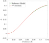 |
Fig. A.1. Ledoux discriminant profile of a reconstructed and reference model, showing the lower reconnection point around 0.08 R⊙. |
Once the A profile in the radiative zone is constructed, the model needs to be reintegrated satisfying hydrostatic equilibrium, mass conservation, and the boundary conditions in mass and radius. From a formal point of view, the equations to reintegrate the structure are expressed as follows:
 (A.1)
(A.1)
 (A.2)
(A.2)
 (A.3)
(A.3)
with the conditions that:  at r = 0; that
  at r = R⊙; and that P = Pref at r = R⊙, where Pref is the surface pressure of the reference model.
The thermal structure of the model was not taken into account and the equations were discretized on a fourth-order finite difference scheme. The system was solved with the help of a Newton-Raphson minimisation, using the reference model as the initial conditions. The final result is a full “acoustic” structure: A, ρ, P, m, and Γ1 built from the A inversion of a given model. From this “acoustic” structure, linear adiabatic oscillation can be computed and the process reiterated until convergence is reached.
All Tables
Comparison between period spacing values for the seismic models after seven iterations and the reference models values.
Comparison between m0.75 for the seismic models after seven iterations and their corresponding reference models values.
All Figures
|
Fig. 1. Left panel: relative differences in squared adiabatic sound speed between the Sun and Seismic model 10 (Sismo 10). Right panel: relative differences in density between the Sun and Seismic Model 10 (Sismo 10). |
| In the text | |
|
Fig. 2. Left panel: relative differences in entropy proxy, S5/3, between the Sun and Seismic Model 10 (Sismo 10). Right panel: differences in Ledoux discriminant between the Sun and Seismic Model 10 (Sismo 10). |
| In the text | |
|
Fig. 3. Left panel: illustration of the agreement in Ledoux discriminant for the reconstructed models using the reference models of Table 1 as initial conditions. Right panel: illustration of the convergence of the A corrections for successive iterations of the reconstruction procedure in the case of Model 10. |
| In the text | |
|
Fig. 4. Left panel: agreement in relative sound-speed differences for the reconstructed models using the reference models of Table 1 as initial conditions. Right panel: illustration of the convergence of the sound-speed relative differences for successive iterations of the reconstruction procedure in the case of Model 10. |
| In the text | |
|
Fig. 5. Left panel: agreement in relative entropy proxy differences for the reconstructed models using the reference models of Table 1 as initial conditions. Right panel: illustration of the convergence of the entropy proxy relative differences for successive iterations of the reconstruction procedure in the case of Model 10. |
| In the text | |
|
Fig. 6. Left panel: agreement in relative density differences for the reconstructed models using the reference models of Table 1 as initial conditions. Right panel: illustration of the convergence of the density relative differences for successive iterations of the reconstruction procedure in the case of Model 10. |
| In the text | |
|
Fig. 7. Agreement in frequency-separation ratios of low-degree p-modes for six reconstructed models using the corresponding references of Table 1 as initial conditions, as well as reference Model 1 shown as comparison. |
| In the text | |
|
Fig. 8. Left panel: Ledoux discriminant profiles from the reconstruction procedure. The dashed lines illustrate the reference profile of some of the models in Table 1 while the continuous lines show the profile on which the procedure converges (using all reference models). Right panel: same as the left panel but for the Brunt-Väisälä frequency. |
| In the text | |
|
Fig. 9. Sound-speed profile in the core region of the reconstructed model, showing the impact of initial conditions in the deep solar core, that is unconstrained by p-modes. |
| In the text | |
|
Fig. A.1. Ledoux discriminant profile of a reconstructed and reference model, showing the lower reconnection point around 0.08 R⊙. |
| In the text | |
Current usage metrics show cumulative count of Article Views (full-text article views including HTML views, PDF and ePub downloads, according to the available data) and Abstracts Views on Vision4Press platform.
Data correspond to usage on the plateform after 2015. The current usage metrics is available 48-96 hours after online publication and is updated daily on week days.
Initial download of the metrics may take a while.