| Issue |
A&A
Volume 642, October 2020
|
|
|---|---|---|
| Article Number | A189 | |
| Number of page(s) | 14 | |
| Section | Stellar structure and evolution | |
| DOI | https://doi.org/10.1051/0004-6361/202037870 | |
| Published online | 20 October 2020 | |
An investigation of 56Ni shells as the source of early light curve bumps in type Ia supernovae
1
School of Physics, Trinity College Dublin, The University of Dublin, Dublin 2, Ireland
e-mail: This email address is being protected from spambots. You need JavaScript enabled to view it.
2
Astrophysics Research Centre, School of Mathematics and Physics, Queen’s University Belfast, Belfast BT7 1NN, UK
Received:
3
March
2020
Accepted:
21
August
2020
Abstract
An excess of flux (i.e. a bump) in the early light curves of type Ia supernovae has been observed in a handful of cases. Multiple scenarios have been proposed to explain this excess flux. Recently, it has been shown that for at least one object (SN 2018oh) the excess emission observed could be the result of a large amount of 56Ni in the outer ejecta (∼0.03 M⊙). We present a series of model light curves and spectra for ejecta profiles containing 56Ni shells of varying masses (0.01, 0.02, 0.03, and 0.04 M⊙) and widths. We find that even for our lowest mass 56Ni shell, an increase of >2 magnitudes is produced in the bolometric light curve at one day after explosion relative to models without a 56Ni shell. We show that the colour evolution of models with a 56Ni shell differs significantly from those without and shows a colour inversion similar to some double-detonation explosion models. Furthermore, spectra of our 56Ni shell models show that strong suppression of flux between ∼3700–4000 Å close to maximum light appears to be a generic feature for this class of model. Comparing our models to observations of SNe 2017cbv and 2018oh, we show that a 56Ni shell of 0.02–0.04 M⊙ can match shapes of the early optical light curve bumps, but the colour and spectral evolution are in disagreement. Our models also predict a strong UV bump that is not observed. This would indicate that an alternative origin for the flux excess is necessary. In addition, based on existing explosion scenarios, producing such a 56Ni shell in the outer ejecta as required to match the light curve shape, without the presence of additional short-lived radioactive material, may prove challenging. Given that only a small amount of 56Ni in the outer ejecta is required to produce a bump in the light curve, such non-monotonically decreasing 56Ni distributions in the outer ejecta must be rare, if they were to occur at all.
Key words: radiative transfer / supernovae: general
© ESO 2020
1. Introduction
Although there is general consensus that type Ia supernovae (SNe Ia) result from the thermonuclear explosions of white dwarfs in binary systems, there is currently little agreement on the types of systems required or the manner through which these systems explode as supernovae (see e.g. Livio & Mazzali 2018; Wang 2018; Jha et al. 2019; Soker 2019 for recent reviews of SNe Ia). Many of the proposed scenarios broadly reproduce observations surrounding maximum light and therefore it is only through observations at either very late or very early times that differences between the various explosion and progenitor scenarios can be discerned. Particular attention has been paid to obtaining observations within hours to days of the explosion, as these times may show a ‘bump’ in the light curve indicating interaction with a companion star (Kasen 2010) or circumstellar material (Piro & Morozova 2016) or the presence of short-lived radioactive isotopes (Noebauer et al. 2017).
To date, only a handful of objects displaying such bumps have been observed, despite extensive observational effort. Although only a small number of examples are known, these objects show considerable diversity, and subsequently multiple scenarios have been invoked to explain the flux excesses. Although peculiar in its own right, iPTF14atg was the first SN Ia discovered that showed a flux excess at early times: a strong ultraviolet pulse was observed within the first ∼4 days following explosion. Based on the models of Kasen (2010), Cao et al. (2015) argue that this early UV emission was the result of interaction between the SN ejecta and companion star, and therefore iPTF14atg was produced via the single degenerate channel. In contrast, Kromer et al. (2016) argue that the spectral evolution of iPTF14atg is incompatible with this scenario and is instead more similar to the violent merger of two white dwarfs; however, they note that this scenario in itself does not explain the early UV emission. Since the discovery of iPTF14atg, additional objects have been claimed to show early excess emission, including SN 2012cg (Marion et al. 2016), SN 2016jhr (Jiang et al. 2017), and SN 2017cbv (Hosseinzadeh et al. 2017).
Hosseinzadeh et al. (2017) also compare their observations of SN 2017cbv to the interaction models of Kasen (2010) and find the models over-predict the UV luminosity at early times. Given this disagreement, they discuss the possibility that the early excess observed in SN 2017cbv is produced by a bubble of radioactive 56Ni. The resulting 56Ni distribution should have a noticeable impact on the early light curve and could produce the short-lived excess luminosity observed (Piro & Nakar 2013, 2014; Jiang et al. 2018; Maeda et al. 2018).
Indeed, the classical double-detonation explosion scenario (in which a helium shell is accumulated and ignites on the surface of a white dwarf) predicts large amounts of 56Ni and other short-lived radioactive isotopes in the outer ejecta (Livne 1990; Livne & Glasner 1991; Woosley & Weaver 1994). Previous studies have shown how the decay of these isotopes can produce light curve bumps similar to those observed (Noebauer et al. 2017; Jiang et al. 2018). Maeda et al. (2018) investigate how the post-explosion composition of the helium shell (including the amount of 56Ni present) affects the model observables and can result in light curve bumps of varying strengths.
Recently, the exceptionally high cadence light curve of SN 2018oh provided another example of an early flux excess (Li et al. 2019). This bump is investigated in detail by both Shappee et al. (2019) and Dimitriadis et al. (2019), who consider multiple origins including companion or CSM interaction, the double detonation scenario, and the possibility of an irregular 56Ni distribution. Shappee et al. (2019) show that SN 2018oh is reasonably well matched up to ∼3 days after explosion by a model with a well mixed 56Ni distribution, while at later times less mixing is preferred. This would indicate that the 56Ni distribution does not decrease monotonically towards the outer ejecta. Furthermore, Dimitriadis et al. (2019) show light curves from models for which there are two distinct 56Ni regions within the ejecta; the majority of 56Ni resides in the centre and powers the main light curve, while a separate shell (0.03 M⊙) of 56Ni in the outer ejecta powers the initial flux excess. Dimitriadis et al. (2019) find favourable agreement with the light curve shape of this scenario, but prefer an interpretation of interaction based on the colour evolution.
Further motivation for the study of irregular 56Ni distributions comes from supernova remnants. Some SNe Ia remnants show evidence for possible large clumps of iron in the outer ejecta (at these late epochs, radioactive 56Ni has decayed fully to stable 56Fe, e.g. Tsebrenko & Soker 2015; Yamaguchi et al. 2017; Sato et al. 2020). In addition, Sato et al. (2019) argue that the structure observed in X-ray images of SNe Ia remnants results from an initially clumpy structure to the explosion itself. The effect of similar clumps on the early light curve however has not been fully explored.
For the first time, we present spectra and light curves resulting from Chandrasekhar-mass models with a shell of 56Ni in the outer ejecta. We compare our radiative transfer models to SNe 2018oh and 2017cbv, for which non-monotonic 56Ni distributions have been considered as possible causes of the observed early excesses, and explore the parameter space that could provide reasonable agreement to both objects. In Sect. 2 we outline the construction of our models. We compare the effects of our non-monotonic 56Ni to models with a smoothly varying 56Ni distribution in Sect. 3.1 and to models with extended 56Ni distributions in Sect. 3.2. A comparison with observations is presented in Sect. 4 along with discussion in Sect. 5. Finally, we present our conclusions in Sect. 6.
2. Models
2.1. Radiative-transfer modelling
All model light curves and spectra presented in this work were calculated using TURTLS (Magee et al. 2018) and are available on GitHub1. In what follows we provide a brief overview of TURTLS. We refer the reader to Magee et al. (2018) for a full description of the code and Magee et al. (2020) for an application. TURTLS is a one-dimensional Monte Carlo radiative transfer code designed for modelling the early time evolution of SNe Ia. The density and composition of the SN ejecta are taken as input parameters and freely defined by the user in a series of discrete cells. Monte Carlo packets representing bundles of photons are injected into the model, tracing the decay of 56Ni. The propagation of these packets is followed throughout the model ejecta for a series of logarithmically separated time steps. For the models presented in this work, simulations are calculated between 0.5 and 30 days after explosion. We limit our simulations to 30 days after explosion due to the assumption of local-thermodynamic equilibrium. Packets are initially injected as γ-packets, representing γ-ray photons, and are followed assuming a γ-ray opacity of 0.03 cm2 g−1. After an interaction with the ejecta, γ-packets are converted to r-packets, representing optical photons. To follow the propagation of r-packets, we use TARDIS (Kerzendorf & Sim 2014; Kerzendorf et al. 2018) to calculate the non-grey expansion opacities in each cell during each time step and also include the effects of electron scattering. Packets emerging from the model region are binned in terms of the time and frequency with which they escaped to construct synthetic observables. Light curves are constructed via a convolution of emerging packet luminosities and the desired set of filter functions.
In order to improve the signal-to-noise ratio of our synthetic observables during the crucial early phases, we implemented into TURTLS the event-based technique (EBT) for spectrum extraction with virtual packets (see Long & Knigge 2002; Sim et al. 2010; Kerzendorf & Sim 2014; Bulla et al. 2015). Briefly, in the EBT, after a Monte Carlo packet performs an interaction with the model ejecta, a given number of “virtual packets” (v-packets) are spawned. Each v-packet is emitted in a random direction with the same frequency in the fluid-frame as the real packets. Once injected, v-packets follow the same computational procedure as real packets, with the exception being that they do not interact with the ejecta. At time step t, an escaping v-packet contributes luminosity, Lν, to the spectrum, which is given by:
 (1)
(1)
where E is the energy of the real packet that spawned the v-packet, N is the number of v-packets created for each real packet, Δt is the width of the time step, Δν is the width of the frequency bin, and τ is the total optical depth accumulated along the trajectory of the virtual packet. In this way, a ‘virtual’ spectrum is created from these packets for each time step in the simulation. The virtual light curve at this time is then calculated by integrating the convolution of this spectrum and the filter functions. This method has previously been shown to reproduce the synthetic observables calculated by direct binning of the real packets (see e.g. Fig. 4 of Kerzendorf & Sim 2014 or Fig. 8 of Bulla et al. 2015). In Fig. 1 we show the dramatic increase in the signal-to-noise ratio of our synthetic spectra using v-packets compared to the direct counting of emerging r-packets.
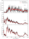 |
Fig. 1. Comparison of spectra calculated during different time steps (1.5 d, 11.0 d, and 18.7 d) for our fiducial SN 2018oh model (see Sect. 2). Virtual spectra (red) are calculated using the event-based technique, while real spectra (black) are calculated by directly counting the luminosities of escaping real packets. |
2.2. Constructing models with 56Ni shells
Dimitriadis et al. (2019) argue that the flux excess observed in the early light curve of SN 2018oh is consistent with a model containing two distinct regions of 56Ni in the ejecta. In this model, the main rise of the light curve is provided by the majority of 56Ni, which is located within the centre of the ejecta. An additional 0.03 M⊙ of 56Ni is placed near the surface of the ejecta (above a mass coordinate of 1.3 M⊙) and powers the initial excess. Following from Dimitriadis et al. (2019), we investigated the range of parameters that could plausibly reproduce the excesses observed in SNe 2018oh and 2017cbv.
As a starting point, we used the models presented in Magee et al. (2020). One of the main limitations of these models is the composition, which uses a simplified three-zone structure (see Fig. 4 of Magee et al. 2018). As the models were designed to explore solely the effects of the 56Ni distribution on the light curve, 56Ni constitutes 100% of the iron-group element (IGE) zone (the centre of the ejecta) immediately after explosion. A small amount (∼0.1 M⊙) of carbon and oxygen was placed in the outer ejecta, while the remaining mass was filled-in with intermediate-mass elements (IME). Due to these limitations, spectra in particular do not provide perfect agreement with observations, as they are more sensitive to specifics of the ejecta composition. The relatively large fraction of IMEs at high velocities for the models presented here is typically reflected in the spectra, with the corresponding features being shifted to higher velocities. Nevertheless, the differences between all models still represent a useful point of comparison. More physical and detailed composition treatments will be explored in future work. Furthermore, all models presented as part of this work have a total ejecta mass of 1.4 M⊙.
To investigate the effects of 56Ni shells on the observables of both objects, we first found models from the existing set presented by Magee et al. (2020) that produced reasonable agreement with the later light curves. We considered these the fiducial models and subsequently added 56Ni shells into the ejecta to determine whether this can reproduce the light curve bump. In determining the fiducial model, we followed the procedure outlined by Magee et al. (2020), but exclude observations > 14 d before B-band maximum. Excluding these early points, we ignored the bump for both SNe and were only concerned with the main rise of the light curve, which will be primarily driven by the 56Ni produced in the core. For SN 2018oh, we find that the Magee et al. (2020) model with 0.6 M⊙ of 56Ni, an exponential density profile, kinetic energy of 1.68 × 1051 erg, and intermediate 56Ni distribution (s = 9.7 in Eq. (5) of Magee et al. 2020) produced good agreement with the light curve beginning approximately five days after explosion. For SN 2017cbv, we find good agreement with a slightly higher 56Ni mass (0.8 M⊙) and lower kinetic energy (1.10 × 1051 erg). Taking these as our fiducial models, we added shells of pure 56Ni into the outer ejecta at different locations, varying the total 56Ni mass of the shell and its width.
The general form of the 56Ni mass fraction within each shell follows a Gaussian distribution, with the 56Ni fraction at mass coordinate m given by
 (2)
(2)
where μ is the centre of the 56Ni shell in M⊙, σ is the width of the shell in M⊙, and A is a dimensionless scaling parameter used to control the total mass of 56Ni in the shell. This mass fraction is then added to the underlying fiducial model to give a description for the entire ejecta. The choice of a Gaussian distribution for the 56Ni mass fraction is arbitrary; however, we have also tested additional functional forms, such as those that are more similar to the inner regions of the ejecta (see Eq. (11) of Magee et al. 2018). We find that the Gaussian distributions produce light curves that more closely resemble SNe 2018oh and SN 2017cbv, and therefore focus on these cases.
In Fig. 2 we show some of the model 56Ni distributions explored as part of this work. As shown in Fig. 2, given that our models are in one dimension, the 56Ni shells would be similar to models containing large amounts of 56Ni in the outer ejecta only along a certain viewing angle. As each of our models has a corresponding fiducial model (i.e. a model without a 56Ni shell), we may consider the difference between the two to qualitatively reproduce the variation along different lines of sight. In this sense, our set of models broadly approximate the effect of a three-dimensional simulation with a large-scale clump of 56Ni visible along a specific line of sight (see Sect. 5 for further discussion).
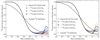 |
Fig. 2. 56Ni distributions for models explored as part of this work. Panels show the best matching models to the light curves beginning approximately five days after explosion (i.e. excluding the early bump) of SN 2018oh (left) and SN 2017cbv (right) as black solid lines, which we consider as our fiducial models. Dashed black lines show models that have more extended 56Ni distributions compared to our fiducial models, but are otherwise identical (i.e. the same density profile and 56Ni mass in each case). Coloured lines show 56Ni shells of varying masses. Each shell is centred on a mass coordinate of 1.35 M⊙ and has a width of either 0.06 or 0.18 M⊙. |
We calculated light curves for 56Ni shells of 0.01, 0.02, 0.03, and 0.04 M⊙, with widths (σ) of 0.06 and 0.18 M⊙ and central locations of 1.35, 1.37, and 1.39 M⊙. In general, we find that changing the central location of the 56Ni shell had little effect on the overall light curve shape. Shells located further out in the ejecta (e.g. at 1.37 or 1.39 M⊙) produced earlier light curve bumps and redder colours beginning a few days after explosion, relative to shells that are somewhat deeper inside the ejecta (e.g. at 1.35 M⊙). The overall effect however, is secondary to the mass and width of the shell. We therefore focus on models with 56Ni shells centred on 1.35 M⊙ as these models produced the best agreement with observations (see Sect. 4) and are representative of the general trends.
As a further point of comparison, we also include models with extended 56Ni distributions relative to the fiducial models. A key feature of our more extended 56Ni distribution models is that the 56Ni mass fraction is always monotonically decreasing towards the outer ejecta. This is clearly not the case for our 56Ni shell models, which have decreasing 56Ni mass fractions below 1.35 M⊙ before increasing again around ∼1 M⊙.
3. Model observables
3.1. Effects of 56Ni shells
In the following section we discuss generally the impact of 56Ni shells on the synthetic observables of the models. Here, we limit this discussion to a comparison between those models with 56Ni shells and those without. In Sect. 3.2, we discuss these models further alongside comparisons to a model with an extended 56Ni distribution relative to our fiducial SN 2018oh model. In Sect. 4, we compare our shell models to observations of SNe 2018oh and 2017cbv and further discuss the implications for their specific explosion scenarios. We focus our discussion here on models in which shells have been added to the fiducial model for SN 2018oh (EXP_Ni0.6_KE1.68_P9.7; see Magee et al. 2020 for further details on the model naming scheme). We find similar trends for models based on the SN 2017cbv fiducial model (EXP_Ni0.8_KE1.10_P9.7). Both of our fiducial models represent intermediate values for the density profile and 56Ni distribution among the full parameter space explored in Magee et al. (2020).
Figures 3a, b, and c demonstrate the effect of 56Ni shells on the bolometric and BR band magnitudes compared to models without shells. We find that while the small increase in total 56Ni mass does not strongly affect the peak absolute magnitude of the models, there are significant differences during the first few days after explosion. For all of the parameters investigated here, an excess of flux in the light curve (relative to the fiducial model) is produced during this time – the duration and total amount of flux excess varies. Again, we note that although our simulations are all performed in one dimension, differences between models with shells and our fiducial models are qualitatively similar to the variation in observables that may be expected along different lines of sight for a multi-dimensional model containing a clump only along a specific viewing angle.
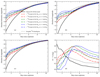 |
Fig. 3. Light curves for models with and without shells of 56Ni in the outer ejecta. Panels a, b, and c show the bolometric, B-, and R-band magnitudes, respectively. The B − V colour evolution is shown in Panel d. We determine our fiducial model for SN 2018oh by finding the best match to the later light curve (excluding the early bump) among the models of Magee et al. (2020). This is shown as a black solid line. Coloured lines show light curves resulting from models with added shells of 56Ni in the outer ejecta, of varying masses. Each shell is centred on a mass coordinate of 1.35 M⊙ and has a width of either 0.06 or 0.18 M⊙. Dashed black lines show a model that has a more extended 56Ni distributions compared to our fiducial model, but is otherwise identical (i.e. the same density profile and 56Ni mass in each case). Our models demonstrate that bumps in the early light curves, of varying sizes and lengths, can be generated by different shells of 56Ni in the outer ejecta. |
We find that in all cases of 56Ni shells, the flux excess is most easily observed in the bluer bands – a natural consequence of the higher temperatures produced in the outer ejecta due to the presence of additional 56Ni heating. For example, in the case of our models with a 0.03 M⊙ 56Ni shell, the B-band is ≳4 mag brighter relative to our fiducial model at approximately one day after explosion. The R-band shows a slightly more modest increase of ∼3 magnitudes. Even for our lowest 56Ni mass shell (0.01 M⊙), the light curves are brighter relative to the fiducial model by ∼3–3.5 mag and ∼2–2.5 mag in the B- and R-bands, respectively. Aside from the total 56Ni mass contained within the shell, the distribution also affects the shape and colour of the flux excess. As shown in Fig. 3, those models with narrower 56Ni shells (σ = 0.06 M⊙) typically show larger and bluer excesses over those models containing broader 56Ni shells (σ = 0.18 M⊙). In addition, they show a somewhat more well-defined peak or bump – broader 56Ni shells generally result in broader light curves with a “shoulder” rather than a distinct bump.
For the models presented here, the duration of the flux excess ranges from ∼4–5 days following explosion. Although the excess may have subsided at later times, the implications for the rest of the time evolution are profound and in particular the colour evolution for models with 56Ni shells differs significantly from those without, as shown in Fig. 3d. For our fiducial model, the initial colour at one day after explosion is quite red (B − V ∼ 0.8 mag) due to a lack of 56Ni in the outer ejecta, but gradually becomes steadily bluer over the next week. Between 7 and 10 days after explosion, the B − V colour has flattened and remains roughly constant at B − V ∼ 0.1. In contrast, models with 56Ni shells show bluer colours (by ∼0.3–0.5 mag) within the first few days after explosion. By ∼4–5 days following explosion, the 56Ni shell models have become significantly redder than the fiducial model, by as much as ∼0.6 mag. The 56Ni shell models subsequently become bluer again, but remain consistently redder than the fiducial model – ranging from ∼0.1–0.4 mag redder around maximum light.
In Fig. 4 we show spectra for our models at 1.50 d and 18.75 d after explosion. These phases correspond to approximately near the peak of the early flux excess and close to maximum light. We focus here on the case of our fiducial SN 2018oh model, models with 56Ni shells of 0.01 and 0.03 M⊙, shell widths of σ = 0.06 M⊙, and a more extended 56Ni distribution relative to the fiducial model. As expected from the differences in light curves and colours at early times (Fig. 3), Fig. 4 shows that the spectra for our 0.03 M⊙ 56Ni shell model are significantly brighter and bluer than all other models at 1.50 d after explosion. At this time, the light curve of our 0.01 M⊙ model is not unlike that of the extended 56Ni distribution model, hence their spectra are also quite similar. In contrast, the lack of 56Ni in the outer ejecta of our fiducial model produces a relatively flat and red spectrum, with the only prominent absorption feature appearing around ∼4800 Å. We note that in Fig. 4, the 1.50 d spectrum of our fiducial model is scaled up by a factor of three to highlight the differences in spectroscopic features.
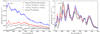 |
Fig. 4. Spectra for models with and without shells of 56Ni in the outer ejecta. Left: spectra are shown for 1.50 d after explosion, which corresponds to during the flux excess phase. All spectra have been binned to Δλ = 15 Å. We note that the spectrum of our fiducial model has been artificially scaled in flux by a factor of three. Right: spectra are shown for 18.75 d after explosion, corresponding to close to maximum light. All spectra have been binned to Δλ = 10 Å. |
In order to determine which elements are responsible for producing the features observed in the spectra, we tracked the opacity bin with which each packet experienced its last interaction and the contribution of each element to the total opacity within this bin. When packets were then binned in frequency to produce the spectrum, this gave the contribution of each element to the total luminosity at a given wavelength (see e.g. Fig. 2 of Kromer & Sim 2009 and Fig. 8 of Magee et al. 2016). This is shown in Fig. 5 for our 1.50 d spectra, where each element is denoted by a different colour. Figure 5 shows that the feature around ∼4800 Å could likely be attributed to Mg II. At all other wavelengths there does not appear to be a dominant source of opacity, hence the last element with which a packet experienced an interaction is approximately random and there is a lack of features in the spectrum. For our model with a 0.03 M⊙ 56Ni shell, Fig. 5 shows that Ni is the dominant source of opacity at all wavelengths. This is unsurprising given that most packets escaping at this time will have originated from the 56Ni shell.
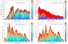 |
Fig. 5. Contribution of individual elements within the model ejecta to the flux at each wavelength. Element fluxes are calculated based on their contribution to the opacity bin with which escaping Monte Carlo packets experienced their last interaction. Spectra are shown for our fiducial model (left) and our model that includes an additional 56Ni shell of 0.03 M⊙ and width of 0.06 M⊙ (right). Spectra are also shown for 1.50 d after explosion, binned to Δλ = 15 Å (top), and 18.75 d after explosion, binned to Δλ = 10 Å (bottom). |
Closer to maximum light, at 18.75 d after explosion, differences in spectra between the models are more subtle, as demonstrated by Fig. 4. We again note that limitations in the composition of our models can result in velocities of IMEs that are too high. For the models shown in Fig. 4, the Si IIλ6355 velocity is ∼15 000 km s−1 at maximum light, while the velocity in SN 2018oh is ∼10 300 km s−1 (Li et al. 2019). In Fig. 5, we also show the contribution of each element to the luminosity at every wavelength for our fiducial model and model with a 0.03 M⊙ 56Ni shell. For all models, we find that the Si IIλ6 355 feature is unaffected by the presence of 56Ni shells. Indeed, wavelengths longer than ∼4500 Å show only small variations at this time. A prominent exception to this is the S II “W” feature around ∼5400 Å. Figure 5 indicates that this feature has become affected by the presence of additional Fe in all but our fiducial model. The most noticeable differences for our model spectra around maximum light occur at wavelengths ≲4500 Å. Figure 5 shows that the strong Ca II H&K features are either significantly weakened or completely removed by the presence of additional IGEs.
Even for relatively small 56Ni shell of 0.01 M⊙ (representing ≲2% of the total 56Ni mass for the models in Fig. 3), a dramatic increase in luminosity at early times can be achieved. Such signatures should be easily detected in observations of SNe Ia, provided they are discovered sufficiently early (within ∼3 days of explosion).
3.2. 56Ni shells versus extended 56Ni distributions
In Fig. 3 we also show comparisons of our 56Ni shell models to a model with a more extended 56Ni distribution relative to our fiducial model. In this case, the 56Ni distribution in the outer ∼0.1 M⊙ is comparable to our 0.01 M⊙ shell model with σ = 0.18 M⊙. Deeper inside the ejecta however, the 56Ni distributions differ significantly. Figure 3 clearly shows the consequences of these differences in 56Ni distributions.
Our extended 56Ni distribution model shows a broad light curve that smoothly increases in brightness towards maximum light. For our 0.01 M⊙ shell model with σ = 0.18 M⊙, the light curve is similar to that of the extended 56Ni distribution model until ∼1.5 days after explosion. After this point, the two models clearly diverge. The shell model shows a somewhat flattening of the rise between ∼1.5–3 days, before subsequently rising more sharply again until maximum light. The colour evolution also differs significantly for both models, as shown in Fig. 3d. The shell model is easily distinguished based on the sudden shift towards redder colours following explosion, while our extended 56Ni distribution model shows a relatively flat colour evolution during the first 10 days post-explosion.
The spectra of our extended 56Ni distribution model are also shown in Fig. 4. At both early times and close to maximum light, the extended 56Ni distribution model appears similar to our 0.01 M⊙ 56Ni shell model. This further highlights the need for continuous follow up as both models are reasonably indistinguishable without observations towards the end of the bump phase (∼2–4 d after explosion).
As discussed in Magee et al. (2020), a light curve bump cannot be produced solely by having a large fraction of 56Ni in the outer ejecta. Our models clearly demonstrate that a bump in the light curve requires the 56Ni distribution to vary non-monotonically. A smoothly decreasing 56Ni fraction towards the outer ejecta will only vary the width and colours of the light curve, but does not produce a flux excess resembling those of models with 56Ni shells. If the shell is extended over a relatively large region of the ejecta (∼0.18 M⊙), a broader light curve can be produced, but even in this case the model is clearly distinguished from a monotonically decreasing extended 56Ni distribution based on the colour evolution.
4. Comparisons with observations of SNe Ia
4.1. SN 2018oh
In the following section, we compare our model light curves and spectra to observations of SN 2018oh. We find the best agreement when assuming an explosion date of MJD = 58144.1 and distance modulus of μ = 33.66 mag and adopt these values throughout this work. We note that the explosion date found here is 0.2 d earlier than the first-light time derived by Li et al. (2019) and the distance modulus is fully consistent. The spectrum of SN 2018oh has been corrected for galactic extinction only (host reddening is estimated to be negligible; Li et al. 2019) and was obtained from WISeREP (Yaron & Gal-Yam 2012). In order to ensure accurate flux calibration, we calculated synthetic magnitudes from the spectrum. We then calculated the offset relative to co-temporal photometric magnitudes and applied this across all bands using a third-order polynomial. The observed spectrum was then scaled to match the photometry in each band.
In Fig. 6, we show a comparison between our models and observations of SN 2018oh. As demonstrated by Fig. 6, our fiducial model provides good agreement with the light curve beginning approximately one week after explosion, but is clearly significantly fainter than the observations at early times. Extending the 56Ni distribution of our fiducial model, such that 56Ni is present throughout the ejecta (see Fig. 2), does not reproduce the shape of the light curve and instead results in a broader light curve that passes through the early flux excess. As in Magee et al. (2020), this indicates that the early excess is not simply due to a large fraction of 56Ni in the outer ejecta.
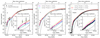 |
Fig. 6. Comparison of SN 2018oh to models with and without 56Ni shells in the outer ejecta. From left to right, panels shown the g-, V-, and Kepler-bands. Observations of SN 2018oh are shown as black points. Non-detections and detections of < 3σ are shown as downward triangles. Our fiducial model is shown as a grey solid line, while models with 56Ni shells are shown as coloured lines. Based on comparisons to our models, we infer an explosion date of MJD = 58144.1, which is shown as a vertical dash-dot line. A model with an extended 56Ni distribution relative to our fiducial SN 2018oh model is shown as a dashed line. The epoch of our spectral comparison is shown as a vertical dotted line. In each panel we show a zoom-in of the first four days after explosion. We note that this does not cover the epoch of the spectral comparison. |
Rather than a simple extended 56Ni distribution, Fig. 6 shows that models with 56Ni shells can broadly reproduce the light curve shape of SN 2018oh throughout its evolution to maximum light. The mass of the 56Ni shell required to match the flux excess of SN 2018oh is between 0.02–0.03 M⊙. This is consistent with the value found by Dimitriadis et al. (2019), although we note that differences in the total 56Ni mass and distribution, and density profile compared to our models likely accounts for differences in the overall light curve shapes. Less massive 56Ni shells (0.01 M⊙) do not reach the required luminosities to match the flux excess around ∼2 days after explosion.
Aside from the mass of the 56Ni shell, there is some tension between the g- (3800 Å ≲ λ ≲ 5400 Å) and Kepler- (4200 Å ≲ λ ≲ 9000 Å) bands over the width of the shell that is required. We find that our model with a narrow (σ = 0.06 M⊙) 0.03 M⊙ shell produces the best match to the g-band light curve of SN 2018oh, while in the Kepler-band the model is somewhat too bright (by ≲0.5 mag) during the excess phase. For the other models shown in Fig. 6, we find broad shells (σ = 0.18 M⊙) generally produce better agreement with the shape of the Kepler light curve, but are slightly fainter than the g-band observations. In addition, our models with 56Ni shells are systematically brighter than the V-band observations around maximum light, while our fiducial model shows better agreement.
These discrepancies are further highlighted by the colour (Fig. 7) and spectral evolution (Fig. 8). Figure 8 shows that even for our fiducial model there is disagreement between the model and observed spectra. This can be attributed to the simplified composition used which, as discussed in Sects. 2 and 3.1, results in IME velocities that are too high. Regardless of these shortcomings, Fig. 4 shows that spectral features at longer wavelengths are largely unaffected by the presence of shells, while shorter wavelengths are much more sensitive. Therefore, comparisons between our shell and fiducial models, and SN 2018oh, are still useful for inferring the effect of 56Ni shells on spectra, and investigating whether any specific signatures they might have at shorter wavelengths are present in SN 2018oh.
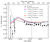 |
Fig. 7. Colour evolution of SN 2018oh compared to models with and without 56Ni shells in the outer ejecta. Observations of SN 2018oh are shown as black points. Our fiducial model is shown as a solid grey line. Models with additional 56Ni shells are shown as coloured lines and our model with an extended 56Ni distribution relative to our fiducial model is shown as a grey dashed line. Based on comparisons to our models, we infer an explosion date of MJD = 58144.1, which is shown as a vertical dash-dot line. The epoch of our spectral comparison is shown as a vertical dotted line. |
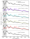 |
Fig. 8. Spectral comparison between SN 2018oh (black) and our models 11 days after explosion. Each spectrum is offset vertically for clarity, with a dashed line showing the zero-point for each offset. The region showing strong flux suppression in our shell models is given by a shaded grey region. Ca II H&K and Si IIλ3858 lines are denoted by vertical dotted lines. |
Shortly after explosion, Fig. 7 shows that our fiducial model is significantly redder than SN 2018oh, in addition to being fainter. The presence of the 56Ni shell provides an additional heating source in those models, and hence their bluer colours are more similar to SN 2018oh at this time (although we note the large uncertainties). Unfortunately, g-band observations are unavailable for the period MJD = 58148–58151 (∼3.8–6.8 d post-explosion), which coincides with the largest discrepancies in colour between our fiducial and 56Ni shell models.
This difference in colour is further reflected in the spectrum at approximately 11.5 d after explosion. For our fiducial model, although the region around ∼3500–4000 Å (shaded in Fig. 8) is fainter than SN 2018oh, the overall shapes of the features are quite similar – with the exception being that the Ca II H&K and Si IIλ3858 lines are blended in our model (dotted lines in Fig. 8). This is clearly not the case in all of our other models however, which show a significant amount of line blanketing. As discussed in Sect. 3, for all models with 56Ni shell there is a strong suppression of flux at wavelengths ≲4500 Å, which can be attributed to the presence of additional IGEs. In addition, all models with 56Ni shells show a relatively flat feature between ∼3700–4000 Å that is not seen in SN 2018oh, or indeed even the model with an extended 56Ni distribution.
Following the colour evolution to maximum light, our shell models reach an inversion shortly before two weeks after explosion. At this point, the colour flattens before gradually becoming increasingly red. Again, this can be attributed to the presence of the 56Ni shell causing an increasing amount of blanketing as more flux emerges from the inner regions of the ejecta. Conversely, our fiducial model does not become as red as the shell models, although it remains redder than SN 2018oh by ∼0.05 mag.
Based on comparisons with observations of SN 2018oh, our models indicate that while 56Ni shells of ∼0.02–0.03 M⊙ can reproduce the early light curve shape there is an overall negative effect on the spectra closer to maximum light. While some differences in features between our models and observations can be attributed to the simple composition used, a strong suppression of flux in the region ∼3700–4000 Å appears to be a generic feature of models with relatively massive 56Ni shells (massive enough to match the early flux excess in the light curve). A similar feature is not observed in SN 2018oh and therefore would suggest that such shells are not present in the outer ejecta. Figure 7 also clearly demonstrates the need for continuous and well-sampled multi-band follow-up of SNe Ia, as the shape of the colour evolution can provide a key diagnostic between the different ejecta structures.
4.2. SN 2017cbv
We now look to compare our models to observations of SN 2017cbv. Here we assume an explosion date of MJD = 57821.2 and distance modulus of μ = 30.74. The distance modulus used in this work is consistent with that of Hosseinzadeh et al. (2017), while the explosion date is 0.7 days earlier. Spectra of SN 2017cbv were corrected for galactic extinction only (host reddening is estimated to be negligible; Hosseinzadeh et al. 2017), obtained from WISeREP (Yaron & Gal-Yam 2012), and originally published in Hosseinzadeh et al. (2017). Spectra were flux calibrated in the same manner as described for SN 2018oh (see Sect. 4.1).
A comparison between the light curves of SN 2017cbv (Hosseinzadeh et al. 2017) and our models is shown in Fig. 9. Figure 9 demonstrates that our fiducial model generally provides reasonable agreement with SN 2017cbv close to maximum light across the optical bands. For the UV bands (UVW2, UVM2, UVW1, and U) however, our fiducial model peaks earlier and fainter than the UV observations. As mentioned previously, we have assumed 56Ni constitutes 100% of the total IGE immediately following explosion. The UV bands are more highly sensitive to the chosen metallicity of the ejecta. A more detailed composition and structure of the ejecta may result in improved agreement. The effect of metallicity on the model observables will be more fully explored in future work.
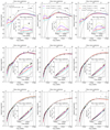 |
Fig. 9. Comparison of SN 2017cbv light curves to models with and without 56Ni shells in the outer ejecta. SN 2017cbv is shown as black points. The fiducial model for SN 2017cbv is shown as a solid grey line. Models with 56Ni shells added to the fiducial model are shown as coloured lines. Based on comparisons to our models, we infer an explosion date of MJD = 57821.2, which is shown as a vertical dash-dot line. A model with an extended 56Ni distribution relative to our fiducial SN 2017cbv model is shown as a dashed line. The epochs of our spectral comparisons are shown as vertical dotted lines. In each panel we show a zoom-in of the first four days after explosion. |
Figure 9 shows that models with 56Ni shells in the outer ejecta can also provide reasonable agreement with the early light curve shape of SN 2017cbv. We find models with 56Ni shells of 0.03–0.04 M⊙ provide the best match to the shape of the BVgri band light curves within the days following explosion. The overall level of agreement in these bands is generally insensitive to the width of the 56Ni shell, but this is clearly not the case for the U-band. Models with narrow 56Ni shells (σ = 0.06 M⊙) reproduce the shape of the U-band flux excess better than those with broader 56Ni shells (σ = 0.18 M⊙), but even in these cases our models show an overall flatter flux excess than observed in SN 2017cbv. In addition, our models predict a strong UV bump within the first few days of explosion that is not observed in SN 2017cbv. Around maximum light, our 56Ni shell models show significant differences compared to our fiducial model and show a much closer resemblance to the extended 56Ni distribution model.
Unlike SN 2018oh, SN 2017cbv has well sampled multi-band observations and spectra extending from explosion to after maximum light and therefore provides a better opportunity to determine which models can be excluded. Here, we consider spectra at three important epochs during the evolution of SN 2017cbv – shortly after explosion (+1.5 d), towards the end of the flux excess phase (+3.5 d), and close to maximum light (+18.5 d). As with SN 2018oh, we find that our fiducial model does not provide perfect agreement at maximum light. We again note that the effect of the shell is most pronounced at shorter wavelengths, while longer wavelengths are less affected (such as the Si IIλ6 355 feature). We therefore focus our spectral comparisons on investigating signatures of the shells at shorter wavelengths.
In Fig. 10 we show the colour evolution (B − V and g − r) of SN 2017cbv compared to our models. Immediately following explosion, our fiducial model is clearly significantly redder than SN 2017cbv, and also shows no prominent features in its spectra (Fig. 11). Those models with narrow 56Ni shells (σ = 0.06 M⊙) provide better agreement with the colour evolution during these epochs. Figure 11 shows that at 1.5 d after explosion the features around ∼3600 and 4200 Å in SN 2017cbv are reasonably well matched by our narrow 56Ni shell models, although the models show a velocity that is too low. By 3.5 d, we also find that the colours and spectroscopic features of some of our shell models are similar, although again the velocities of IGE features are too low in the model. Better agreement may be achieved if the density profile was altered such that the 56Ni shell was shifted to higher velocities.
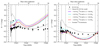 |
Fig. 10. Comparison of the B − V (left) and g − r (right) colour evolution in SN 2017cbv (black points) to models with (coloured lines) and without 56Ni shells (grey lines) in the outer ejecta. A model with an extended 56Ni distribution relative to our fiducial SN 2017cbv model is shown as a dashed line. The epochs of our spectral comparisons are shown as vertical dotted lines. |
After these early phases the initial light curve bump has subsided and the colour evolution of SN 2017cbv shows a small increase to redder colours until approximately one week after explosion. At this point the evolution turns towards bluer colours again. Our fiducial and extended 56Ni distribution models (i.e. those models without 56Ni shells) clearly do not match the shape of this colour evolution. Initially their colours are very red and become increasingly blue, and then steadily becoming redder again from approximately one week after explosion. In contrast, our 56Ni shell models show a similar colour inversion as in SN 2017cbv, although the colours are systematically shifted redder by ∼0.2 mag. Models with narrower 56Ni shells also typically show more dramatic changes in colour than SN 2017cbv. For example, over approximately five days, SN 2017cbv shows a shift of Δ(B − V)∼0.1 mag. This is similar to the colour change in our broader 56Ni shell models, but significantly smaller than that of our narrow 56Ni shell models where Δ(B − V)≳0.2 mag. This is clearly in disagreement with the U-band light curve shape and the early spectral comparisons, for which we find better agreement with narrow 56Ni shell.
We note that the g − r colour of SN 2017cbv does not show a similar colour evolution as in the B − V colour during the early epochs. Instead the colour becomes slightly bluer (by ∼0.1 mag) before flattening. In contrast, our 56Ni shell models still show a slight colour inversion. Additionally, the g − r colours of these models are significantly bluer than SN 2017cbv beginning approximately one week after explosion. Instead, the shape of the colour evolution in our fiducial model is more similar to that of SN 2017cbv (although the colours are systematically redder in the model), excluding the initial few days during the flux excess phase.
Although the early light curve shapes are reasonably well reproduced in our 56Ni shell models, it is clear that at maximum light there is significant disagreement, as shown in Fig. 11. As in SN 2018oh, we find that close to maximum light, our models do not reproduce the Ca II H&K and Si IIλ3858 lines. Instead, our models show strong flux suppression in this region due to the presence of additional IGEs. Although at early times it is significantly fainter than SN 2017cbv, our fiducial model provides the best agreement around maximum. As in the case of SN 2018oh, our models show that the flux suppression in the near-UV appears to be a generic feature of models with 56Ni shell. Those models with shells large enough to match the light curve shape all exhibit this feature, which is not observed in the spectra of SN 2017cbv. Therefore, we argue that while a 56Ni shell could explain the observed light curve shape, it is inconsistent with the spectral evolution.
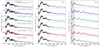 |
Fig. 11. Spectral comparison between SN 2017cbv (black) and our models. From left to right panels show spectra at 1.5, 3.5, and 18.5 days after explosion. Each spectrum is offset vertically for clarity, with a dashed line showing the zero-point for each offset. The region showing strong flux suppression at maximum light in our shell models is given by a shaded grey region. |
5. Discussion
Our models show that 56Ni shells in the outer ejecta can produce an excess of flux during the first few days after explosion – the strength and duration of which depend on both the mass and width of the shell. Comparing our models to observations of SNe 2018oh and 2017cbv, we find that massive (∼0.02–0.04 M⊙) 56Ni shells can in general reproduce the shape of the optical light curve bumps and colours within the first few days of explosion. Such massive shells produce strong flux suppression at near-UV wavelengths however, which is not seen in the spectra of either object. In Sect. 5.1 we first discuss predictions of 56Ni shells from existing explosion models, while in Sect. 5.2 we discuss alternative scenarios for producing early light curve bumps and how they compare to those produced by 56Ni shells.
5.1. Sources of non-monotonic 56Ni distributions in the outer ejecta
As discussed in Sect. 2, our one-dimensional shell models may be considered qualitatively similar to multi-dimensional models in which an excess of 56Ni is produced directly along the line of sight. In other words, the one-dimensional shell is equivalent to a localised clump of 56Ni. Many of the models proposed for SNe Ia invoke deflagrations to some degree, which could provide one method of producing 56Ni clumps (Khokhlov et al. 1993; Hoeflich & Khokhlov 1996; Gamezo et al. 2005; Bravo & García-Senz 2006; Jordan et al. 2008). Generally, in such models the interior of the white dwarf is initially burned by a sub-sonic deflagration. As the burning front propagates, it will eventually become subject to Rayleigh-Taylor instabilities that wrinkle and deform the flame (Khokhlov 1994, 1995). At the same time, buoyancy of the hot, burned ash accelerates the deflagration plumes towards the surface of the white dwarf (Reinecke et al. 2002). The overall effect of the deflagration is irregular or uneven burning, and deflagration plumes could therefore potentially create 56Ni clumps in the outer ejecta. Multi-dimensional simulations in general however, do not show strong variations in the light curves as a function of viewing angle, which may be expected if there were significant differences in composition along certain directions (see e.g. Röpke et al. 2007a; Seitenzahl et al. 2013; Sim et al. 2013; Fink et al. 2014; Long et al. 2014).
One potential scenario for producing large 56Ni clumps in the outer ejecta lies in gravitationally confined detonations (GCDs; Plewa et al. 2004). This scenario does produce an excess that is qualitatively similar to SNe 2018oh and 2017cbv, although much less extreme. Here, the deflagration plumes reach the surface of the white dwarf before burning transitions to a detonation. As the plumes travel along the surface, they eventually converge on the stellar point opposite that of the initial breakout and it is this convergence that triggers the detonation. The result is a highly asymmetric ejecta composition in which clumps of deflagration ash are present at high velocities. Seitenzahl et al. (2016) present light curves and spectra for one realisation of the GCD scenario, which shows a strong dependence on viewing angle. When viewed close to the direction of the deflagration ignition, a small bump (≲0.5 mag and lasting ∼3 days) in the U-band light curve is observed (see Fig. 7 of Seitenzahl et al. 2016), resulting from the presence of the deflagration ash. Whether the GCD scenario could produce larger 56Ni clumps similar to those studied here remains to be seen, but warrants further investigation.
We note that it has also been argued that the GCD scenario may not be robustly achieved (Röpke et al. 2007b) and while initial models designed to mimic the GCD scenario could reproduce observables of SNe Ia (Kasen & Plewa 2005), subsequent multi-dimensional explosion simulations have shown good agreement with neither normal nor 91T-like SNe Ia (Seitenzahl et al. 2016). In addition, the abundance distribution appears dissimilar to that inferred for normal SNe Ia based on late-time spectra (Maguire et al. 2018), as much of the stable material produced in the high density core would be carried to the outer ejecta through buoyancy.
Aside from models invoking deflagrations, the double-detonation scenario is another possibility for producing large 56Ni mass fractions in the outer ejecta (Livne 1990; Woosley & Weaver 1994; Bildsten et al. 2007). In these models, a thin helium shell builds up on the surface of the WD. Depending on certain conditions (e.g. mass of the WD, mass of the helium shell, etc.), the shell may ignite and create a secondary detonation that leads to the complete disruption of the star (Fink et al. 2007). In general, burning in the helium shell can produce a large amount of 56Ni, qualitatively similar to the 56Ni shells included in this work (Fink et al. 2010; Shen et al. 2010; Moll & Woosley 2013). Similar to our models, the presence of a 56Ni shell produces an excess of flux within the days following explosion. The duration and luminosity of this flux excess is affected by both the mass and post-explosion composition of the helium shell, and is comparable to that predicted by our 56Ni shell models (Maeda et al. 2018; Polin et al. 2019). Although some double-detonation models predominantly produce 56Ni during the shell burning, other short-lived radioactive isotopes are also synthesised – in particular 48Cr and 52Fe (Woosley & Weaver 1994). Aside from affecting the light curves, the presence of these additional isotopes also produces a distinctive Ti II (48Ti is a daughter product of the 48Cr decay chain) trough between ∼4000–4300 Å. Even for models in which the helium shell products are dominated by 56Ni, a strong Ti II feature is produced (Polin et al. 2019). The presence of such a feature could therefore provide one method for distinguishing a 56Ni excess produced by helium shell detonations and other methods. Finally, Maeda et al. (2018) present spectra calculated from models with and without helium burning ash, which are qualitatively similar to our models with 56Ni shells and fiducial models. Unlike our models, Maeda et al. (2018) find that spectra of at least some models with helium shells containing 56Ni are redder at three days after explosion than those models without shells. This behaviour is opposite to that of our 56Ni shell models and likely results from the increased line blanketing due to additional elements within the outer ejecta, rather than solely 56Ni as in our models.
Even relatively small 56Ni shells in the outer ejecta (0.01 M⊙ of 56Ni above a mass coordinate of 1.35 M⊙) can have a significant effect on the light curve, producing a light curve bump that increases the bolometric magnitude by > 2 magnitudes at one day after explosion. Given that such bumps are not observed for the majority of SNe Ia, this would indicate that 56Ni shells (at least those large enough to reproduce the light curve shapes of SN 2018oh and SN 2017cbv) must be relatively rare phenomena, if indeed they occur at all.
5.2. Alternative sources of flux excesses
While our models show that 56Ni shells in the outer ejecta can produce an excess of flux at early times, similar behaviour is found for other scenarios that do not invoke the presence of additional 56Ni – in particular, interaction between the SN ejecta and companion star or circumstellar material (CSM). In both cases, this material is shock heated by the SN ejecta and gradually cools, providing an additional source of luminosity.
Kasen (2010) shows how the total luminosity produced during the light curve bump varies depending on the nature of the companion, with larger mass and more evolved companions producing larger flux excesses. For red giant companions, the B-band flux excess is approximately one magnitude fainter than peak, while in the ultraviolet it is approximately one magnitude brighter. This is unlike our 56Ni shell models, in which the flux excess is always ≳2 mag fainter than peak. In contrast, less evolved main sequence stars show flux excesses covering a similar range in magnitude to that of our 56Ni shell models, although they are generally shorter lived. For example, when assuming interaction occurs with a 6 M⊙ MS companion, the B-band light curve has already plateaued within ∼1 day of explosion. The companion interaction scenario has been proposed for the light curve bumps in SNe 2018oh and 2017cbv, and is the favoured interpretation in both cases (Hosseinzadeh et al. 2017; Dimitriadis et al. 2019; Shappee et al. 2019). We note, however, that both SNe show a fainter UV luminosity than predicted by this model and show no signs of hydrogen, which is expected to be swept up during the interaction and produce strong emission at late times (Sand et al. 2018; Tucker et al. 2019).
An early light curve bump may also be produced due to the interaction between the SN ejecta and CSM. This CSM may result from either accretion of a non-degenerate companion or following a merger. In the case of SN 2017cbv however, the presence of CSM from a non-degenerate companion was investigated by Ferretti et al. (2017), who find no evidence for significant amounts of material. Light curve bumps resulting from post-merger CSM interactions were investigated by Piro & Morozova (2016), who show that various light curve bumps can be produced depending on the mass and radial extent of the material. Piro & Morozova (2016) also demonstrate that the distribution of 56Ni within the ejecta plays an important role in shaping the light curve bump, as those models with more extended 56Ni distributions can mask the signatures of interaction. In all cases, those CSM models without mixed 56Ni distributions produce pronounced bumps in the V-band light curve that differ significantly from the shapes of the bumps in our models. For those models with more extended 56Ni distributions, the CSM mass must be relatively large (∼0.3 M⊙) to produce a flux excess as long lived as our 56Ni shell models.
Within the merger scenario, an accretion disk may also be formed around the more massive primary (Levanon et al. 2015). Based on analytical models, Levanon & Soker (2017) show that following the explosion this disk-originated matter (DOM) is shock heated and produces early UV emission. Levanon & Soker (2019) argue that the early light curve bump of SN 2018oh is consistent with interaction between SN ejecta and DOM. The timescale and luminosity of the flux excess produced by the DOM interaction scenario is also similar to some our of 56Ni shell models, and therefore warrants further investigation with full radiative transfer calculations.
6. Conclusions
Following from the works of Dimitriadis et al. (2019) and Shappee et al. (2019), we investigated 56Ni shells in the outer ejecta as a source of the flux excess observed in SNe 2018oh and 2017cbv. For each object, we took a fiducial model that reproduced the later light curve (i.e. ignoring the early flux excess) and added 56Ni shells to investigate the changes relative to a model without a shell. We presented light curves and spectra for models containing 56Ni shells of 0.01–0.04 M⊙. In all cases, we found that models with 56Ni shells produce an excess of flux during the first few days after explosion. Even a relatively small 56Ni shell of 0.01 M⊙ can have a profound effect on the early light curve and produce an increase in the bolometric magnitude >2 mag at one day after explosion. The appearance of the flux excess is also affected by the shape of the 56Ni shell, with narrower shells producing excesses with a more well-defined peak than broader shells. In addition, our models show that the effects of the 56Ni shells are most prominent at shorter wavelengths and the colour evolution of models with 56Ni shells differs significantly. All models with 56Ni shells show an inversion in the B − V colour evolution between ∼3–6 days after explosion and are clearly distinguished from the fiducial models and even models with more extended 56Ni distributions.
We compared the light curves of our models with 56Ni shells to observations of SNe 2018oh and 2017cbv and found improved agreement compared to the fiducial models – our 56Ni shell models can produce the overall light curve shape in both objects. Similar to Dimitriadis et al. (2019), we found that a 56Ni shell of 0.02–0.03 M⊙ is required to reproduce the shape of SN 2018oh, while for SN 2017cbv a slightly higher mass of 0.03–0.04 M⊙ is required. Although our 56Ni shell models can reproduce the early optical light curve bumps of both objects, there are noticeable differences in the colours and spectral evolution. Our models are systematically redder and show more extreme changes in colour than the observations. A strong suppression of flux in the region of ∼3700–4000 Å also appears to be a generic feature in the maximum light spectra of our 56Ni shell models. Neither SN 2018oh nor SN 2017cbv show a similar feature, indicating that while models with 56Ni shells could match the light curve shapes, the spectra are in disagreement. In addition, our 56Ni shell models produce a strong bump in the UV light curves that is not observed. Overall, this would suggest that 56Ni shells are not the source of the early excess flux in either object.
Based on existing explosion models, producing such shells (or clumps) in the outer ejecta as required also appears challenging. The GCD scenario can produce 56Ni clumps in the outer ejecta for certain viewing angles and hence can also produce a small bump in the light curve. Such clumps however, are not as extreme as would be required to match the light curve shapes of SNe 2018oh and 2017cbv. Whether this scenario could produce larger 56Ni clumps and good agreement with observations remains to be seen, but warrants further investigation. Alternatively, the double detonation scenario can also produce large 56Ni fractions in the burned ash of the accreted helium shell. Again, this scenario can also produce light curve bumps, but the picture is complicated by the presence of short-lived isotopes providing an additional powering source for the early light curve. In addition, the helium shell ash produces distinct spectroscopic features, such as strong Ti II absorption. The presence of such a feature could therefore provide one method of distinguishing between 56Ni shells or clumps produced by either deflagration or helium shell ash.
Studies of SNe Ia have shown that early light curve bumps are rare. Only a handful of objects displaying bumps are currently known, despite extensive searches. Based on a sample of 35 SNe Ia with sufficiently early light curves, Magee et al. (2020) find ∼20–30% of objects show evidence for a flux excess when compared against their model light curves. Given that even a relatively small 56Ni shell can significantly alter the light curve shape, this would indicate that non-monotonic 56Ni distributions in the outer ejecta (at least those similar to what is required to match the light curves of SNe 2018oh or 2017cbv) must also be relatively rare – if they occur naturally at all. Future surveys dedicated to the discovery and follow-up of SNe at early times will help to shed light on the nature of flux excesses in SNe Ia.
Acknowledgments
We thank M. Bulla and S. A. Sim for their help in implementing virtual packets into TURTLS. We thank the referees for their suggestions to improve the clarity of the paper. This work was supported by TCHPC (Research IT, Trinity College Dublin). Calculations were performed on the Kelvin cluster maintained by the Trinity Centre for High Performance Computing. This cluster was funded through grants from the Higher Education Authority, through its PRTLI program. This work made use of the Queen’s University Belfast HPC Kelvin cluster. M.M. and K.M. are funded by the EU H2020 ERC Grant no. 758638. This research made use of TARDIS, a community-developed software package for spectral synthesis in supernovae (Kerzendorf & Sim 2014). The development of TARDIS received support from the Google Summer of Code initiative and from ESA’s Summer of Code in Space program. TARDIS makes extensive use of Astropy and PyNE.
References
- Bildsten, L., Shen, K. J., Weinberg, N. N., & Nelemans, G. 2007, ApJ, 662, L95 [NASA ADS] [CrossRef] [Google Scholar]
- Bravo, E., & García-Senz, D. 2006, ApJ, 642, L157 [NASA ADS] [CrossRef] [Google Scholar]
- Bulla, M., Sim, S. A., & Kromer, M. 2015, MNRAS, 450, 967 [NASA ADS] [CrossRef] [Google Scholar]
- Cao, Y., Kulkarni, S. R., Howell, D. A., et al. 2015, Nature, 521, 328 [NASA ADS] [CrossRef] [Google Scholar]
- Dimitriadis, G., Foley, R. J., Rest, A., et al. 2019, ApJ, 870, L1 [NASA ADS] [CrossRef] [Google Scholar]
- Ferretti, R., Amanullah, R., Bulla, M., et al. 2017, ApJ, 851, L43 [CrossRef] [Google Scholar]
- Fink, M., Hillebrandt, W., & Röpke, F. K. 2007, A&A, 476, 1133 [NASA ADS] [CrossRef] [EDP Sciences] [Google Scholar]
- Fink, M., Röpke, F. K., Hillebrandt, W., et al. 2010, A&A, 514, A53 [NASA ADS] [CrossRef] [EDP Sciences] [Google Scholar]
- Fink, M., Kromer, M., Seitenzahl, I. R., et al. 2014, MNRAS, 438, 1762 [NASA ADS] [CrossRef] [Google Scholar]
- Gamezo, V. N., Khokhlov, A. M., & Oran, E. S. 2005, ApJ, 623, 337 [NASA ADS] [CrossRef] [Google Scholar]
- Hoeflich, P., & Khokhlov, A. 1996, ApJ, 457, 500 [NASA ADS] [CrossRef] [Google Scholar]
- Hosseinzadeh, G., Sand, D. J., Valenti, S., et al. 2017, ApJ, 845, L11 [NASA ADS] [CrossRef] [Google Scholar]
- Jha, S. W., Maguire, K., & Sullivan, M. 2019, Nat. Astron., 3, 706 [CrossRef] [Google Scholar]
- Jiang, J.-A., Doi, M., Maeda, K., et al. 2017, Nature, 550, 80 [NASA ADS] [CrossRef] [Google Scholar]
- Jiang, J.-A., Doi, M., Maeda, K., & Shigeyama, T. 2018, ApJ, 865, 149 [NASA ADS] [CrossRef] [Google Scholar]
- Jordan, G. C., IV, Fisher, R. T., Townsley, D. M., et al. 2008, ApJ, 681, 1448 [NASA ADS] [CrossRef] [Google Scholar]
- Kasen, D. 2010, ApJ, 708, 1025 [NASA ADS] [CrossRef] [Google Scholar]
- Kasen, D., & Plewa, T. 2005, ApJ, 622, L41 [NASA ADS] [CrossRef] [Google Scholar]
- Kerzendorf, W., Nöbauer, U., Sim, S., et al. 2018, tardis-sn/tardis: TARDIS v2.0.2 release (Zenodo Software Release) [Google Scholar]
- Kerzendorf, W. E., & Sim, S. A. 2014, MNRAS, 440, 387 [NASA ADS] [CrossRef] [Google Scholar]
- Khokhlov, A. 1994, ApJ, 424, L115 [CrossRef] [Google Scholar]
- Khokhlov, A. M. 1995, ApJ, 449, 695 [NASA ADS] [CrossRef] [Google Scholar]
- Khokhlov, A., Mueller, E., & Hoeflich, P. 1993, A&A, 270, 223 [NASA ADS] [CrossRef] [Google Scholar]
- Kromer, M., & Sim, S. A. 2009, MNRAS, 398, 1809 [Google Scholar]
- Kromer, M., Fremling, C., Pakmor, R., et al. 2016, MNRAS, 459, 4428 [NASA ADS] [CrossRef] [Google Scholar]
- Levanon, N., & Soker, N. 2017, MNRAS, 470, 2510 [CrossRef] [Google Scholar]
- Levanon, N., & Soker, N. 2019, ApJ, 872, L7 [CrossRef] [Google Scholar]
- Levanon, N., Soker, N., & García-Berro, E. 2015, MNRAS, 447, 2803 [NASA ADS] [CrossRef] [Google Scholar]
- Li, W., Wang, X., Vinkó, J., et al. 2019, ApJ, 870, 12 [CrossRef] [Google Scholar]
- Livio, M., & Mazzali, P. 2018, Phys. Rep., 736, 1 [NASA ADS] [CrossRef] [Google Scholar]
- Livne, E. 1990, ApJ, 354, L53 [NASA ADS] [CrossRef] [Google Scholar]
- Livne, E., & Glasner, A. S. 1991, ApJ, 370, 272 [NASA ADS] [CrossRef] [Google Scholar]
- Long, K. S., & Knigge, C. 2002, ApJ, 579, 725 [NASA ADS] [CrossRef] [Google Scholar]
- Long, M., Jordan, G. C., IV, van Rossum, D. R., et al. 2014, ApJ, 789, 103 [NASA ADS] [CrossRef] [Google Scholar]
- Maeda, K., Jiang, J.-A., Shigeyama, T., & Doi, M. 2018, ApJ, 861, 78 [NASA ADS] [CrossRef] [Google Scholar]
- Magee, M. R., Kotak, R., Sim, S. A., et al. 2016, A&A, 589, A89 [NASA ADS] [CrossRef] [EDP Sciences] [Google Scholar]
- Magee, M. R., Sim, S. A., Kotak, R., & Kerzendorf, W. E. 2018, A&A, 614, A115 [NASA ADS] [CrossRef] [EDP Sciences] [Google Scholar]
- Magee, M. R., Maguire, K., Kotak, R., et al. 2020, A&A, 634, A37 [CrossRef] [EDP Sciences] [Google Scholar]
- Maguire, K., Sim, S. A., Shingles, L., et al. 2018, MNRAS, 477, 3567 [NASA ADS] [CrossRef] [Google Scholar]
- Marion, G. H., Brown, P. J., Vinkó, J., et al. 2016, ApJ, 820, 92 [NASA ADS] [CrossRef] [Google Scholar]
- Moll, R., & Woosley, S. E. 2013, ApJ, 774, 137 [NASA ADS] [CrossRef] [Google Scholar]
- Noebauer, U. M., Kromer, M., Taubenberger, S., et al. 2017, MNRAS, 472, 2787 [NASA ADS] [CrossRef] [Google Scholar]
- Piro, A. L., & Nakar, E. 2013, ApJ, 769, 67 [NASA ADS] [CrossRef] [Google Scholar]
- Piro, A. L., & Nakar, E. 2014, ApJ, 784, 85 [NASA ADS] [CrossRef] [Google Scholar]
- Piro, A. L., & Morozova, V. S. 2016, ApJ, 826, 96 [NASA ADS] [CrossRef] [Google Scholar]
- Plewa, T., Calder, A. C., & Lamb, D. Q. 2004, ApJ, 612, L37 [Google Scholar]
- Polin, A., Nugent, P., & Kasen, D. 2019, ApJ, 873, 84 [NASA ADS] [CrossRef] [Google Scholar]
- Reinecke, M., Hillebrandt, W., & Niemeyer, J. C. 2002, A&A, 391, 1167 [NASA ADS] [CrossRef] [EDP Sciences] [Google Scholar]
- Röpke, F. K., Hillebrandt, W., Schmidt, W., et al. 2007a, ApJ, 668, 1132 [NASA ADS] [CrossRef] [Google Scholar]
- Röpke, F. K., Woosley, S. E., & Hillebrandt, W. 2007b, ApJ, 660, 1344 [NASA ADS] [CrossRef] [Google Scholar]
- Sand, D. J., Graham, M. L., Botyánszki, J., et al. 2018, ApJ, 863, 24 [NASA ADS] [CrossRef] [Google Scholar]
- Sato, T., Hughes, J. P., Williams, B. J., & Morii, M. 2019, ApJ, 879, 64 [CrossRef] [Google Scholar]
- Sato, T., Bravo, E., Badenes, C., et al. 2020, ApJ, 890, 104 [CrossRef] [Google Scholar]
- Seitenzahl, I. R., Ciaraldi-Schoolmann, F., Röpke, F. K., et al. 2013, MNRAS, 429, 1156 [Google Scholar]
- Seitenzahl, I. R., Kromer, M., Ohlmann, S. T., et al. 2016, A&A, 592, A57 [NASA ADS] [CrossRef] [EDP Sciences] [Google Scholar]
- Shappee, B. J., Holoien, T. W.-S., Drout, M. R., et al. 2019, ApJ, 870, 13 [NASA ADS] [CrossRef] [Google Scholar]
- Shen, K. J., Kasen, D., Weinberg, N. N., Bildsten, L., & Scannapieco, E. 2010, ApJ, 715, 767 [NASA ADS] [CrossRef] [Google Scholar]
- Sim, S. A., Miller, L., Long, K. S., Turner, T. J., & Reeves, J. N. 2010, MNRAS, 404, 1369 [NASA ADS] [Google Scholar]
- Sim, S. A., Seitenzahl, I. R., Kromer, M., et al. 2013, MNRAS, 436, 333 [NASA ADS] [CrossRef] [Google Scholar]
- Soker, N. 2019, New Astron. Rev., 87, 101535 [CrossRef] [Google Scholar]
- Tsebrenko, D., & Soker, N. 2015, MNRAS, 453, 166 [CrossRef] [Google Scholar]
- Tucker, M. A., Shappee, B. J., & Wisniewski, J. P. 2019, ApJ, 872, L22 [NASA ADS] [CrossRef] [Google Scholar]
- Wang, B. 2018, Res. Astron. Astrophys., 18, 049 [NASA ADS] [CrossRef] [Google Scholar]
- Woosley, S. E., & Weaver, T. A. 1994, ApJ, 423, 371 [Google Scholar]
- Yamaguchi, H., Hughes, J. P., Badenes, C., et al. 2017, ApJ, 834, 124 [CrossRef] [Google Scholar]
- Yaron, O., & Gal-Yam, A. 2012, PASP, 124, 668 [NASA ADS] [CrossRef] [Google Scholar]
All Figures
|
Fig. 1. Comparison of spectra calculated during different time steps (1.5 d, 11.0 d, and 18.7 d) for our fiducial SN 2018oh model (see Sect. 2). Virtual spectra (red) are calculated using the event-based technique, while real spectra (black) are calculated by directly counting the luminosities of escaping real packets. |
| In the text | |
|
Fig. 2. 56Ni distributions for models explored as part of this work. Panels show the best matching models to the light curves beginning approximately five days after explosion (i.e. excluding the early bump) of SN 2018oh (left) and SN 2017cbv (right) as black solid lines, which we consider as our fiducial models. Dashed black lines show models that have more extended 56Ni distributions compared to our fiducial models, but are otherwise identical (i.e. the same density profile and 56Ni mass in each case). Coloured lines show 56Ni shells of varying masses. Each shell is centred on a mass coordinate of 1.35 M⊙ and has a width of either 0.06 or 0.18 M⊙. |
| In the text | |
|
Fig. 3. Light curves for models with and without shells of 56Ni in the outer ejecta. Panels a, b, and c show the bolometric, B-, and R-band magnitudes, respectively. The B − V colour evolution is shown in Panel d. We determine our fiducial model for SN 2018oh by finding the best match to the later light curve (excluding the early bump) among the models of Magee et al. (2020). This is shown as a black solid line. Coloured lines show light curves resulting from models with added shells of 56Ni in the outer ejecta, of varying masses. Each shell is centred on a mass coordinate of 1.35 M⊙ and has a width of either 0.06 or 0.18 M⊙. Dashed black lines show a model that has a more extended 56Ni distributions compared to our fiducial model, but is otherwise identical (i.e. the same density profile and 56Ni mass in each case). Our models demonstrate that bumps in the early light curves, of varying sizes and lengths, can be generated by different shells of 56Ni in the outer ejecta. |
| In the text | |
|
Fig. 4. Spectra for models with and without shells of 56Ni in the outer ejecta. Left: spectra are shown for 1.50 d after explosion, which corresponds to during the flux excess phase. All spectra have been binned to Δλ = 15 Å. We note that the spectrum of our fiducial model has been artificially scaled in flux by a factor of three. Right: spectra are shown for 18.75 d after explosion, corresponding to close to maximum light. All spectra have been binned to Δλ = 10 Å. |
| In the text | |
|
Fig. 5. Contribution of individual elements within the model ejecta to the flux at each wavelength. Element fluxes are calculated based on their contribution to the opacity bin with which escaping Monte Carlo packets experienced their last interaction. Spectra are shown for our fiducial model (left) and our model that includes an additional 56Ni shell of 0.03 M⊙ and width of 0.06 M⊙ (right). Spectra are also shown for 1.50 d after explosion, binned to Δλ = 15 Å (top), and 18.75 d after explosion, binned to Δλ = 10 Å (bottom). |
| In the text | |
|
Fig. 6. Comparison of SN 2018oh to models with and without 56Ni shells in the outer ejecta. From left to right, panels shown the g-, V-, and Kepler-bands. Observations of SN 2018oh are shown as black points. Non-detections and detections of < 3σ are shown as downward triangles. Our fiducial model is shown as a grey solid line, while models with 56Ni shells are shown as coloured lines. Based on comparisons to our models, we infer an explosion date of MJD = 58144.1, which is shown as a vertical dash-dot line. A model with an extended 56Ni distribution relative to our fiducial SN 2018oh model is shown as a dashed line. The epoch of our spectral comparison is shown as a vertical dotted line. In each panel we show a zoom-in of the first four days after explosion. We note that this does not cover the epoch of the spectral comparison. |
| In the text | |
|
Fig. 7. Colour evolution of SN 2018oh compared to models with and without 56Ni shells in the outer ejecta. Observations of SN 2018oh are shown as black points. Our fiducial model is shown as a solid grey line. Models with additional 56Ni shells are shown as coloured lines and our model with an extended 56Ni distribution relative to our fiducial model is shown as a grey dashed line. Based on comparisons to our models, we infer an explosion date of MJD = 58144.1, which is shown as a vertical dash-dot line. The epoch of our spectral comparison is shown as a vertical dotted line. |
| In the text | |
|
Fig. 8. Spectral comparison between SN 2018oh (black) and our models 11 days after explosion. Each spectrum is offset vertically for clarity, with a dashed line showing the zero-point for each offset. The region showing strong flux suppression in our shell models is given by a shaded grey region. Ca II H&K and Si IIλ3858 lines are denoted by vertical dotted lines. |
| In the text | |
|
Fig. 9. Comparison of SN 2017cbv light curves to models with and without 56Ni shells in the outer ejecta. SN 2017cbv is shown as black points. The fiducial model for SN 2017cbv is shown as a solid grey line. Models with 56Ni shells added to the fiducial model are shown as coloured lines. Based on comparisons to our models, we infer an explosion date of MJD = 57821.2, which is shown as a vertical dash-dot line. A model with an extended 56Ni distribution relative to our fiducial SN 2017cbv model is shown as a dashed line. The epochs of our spectral comparisons are shown as vertical dotted lines. In each panel we show a zoom-in of the first four days after explosion. |
| In the text | |
|
Fig. 10. Comparison of the B − V (left) and g − r (right) colour evolution in SN 2017cbv (black points) to models with (coloured lines) and without 56Ni shells (grey lines) in the outer ejecta. A model with an extended 56Ni distribution relative to our fiducial SN 2017cbv model is shown as a dashed line. The epochs of our spectral comparisons are shown as vertical dotted lines. |
| In the text | |
|
Fig. 11. Spectral comparison between SN 2017cbv (black) and our models. From left to right panels show spectra at 1.5, 3.5, and 18.5 days after explosion. Each spectrum is offset vertically for clarity, with a dashed line showing the zero-point for each offset. The region showing strong flux suppression at maximum light in our shell models is given by a shaded grey region. |
| In the text | |
Current usage metrics show cumulative count of Article Views (full-text article views including HTML views, PDF and ePub downloads, according to the available data) and Abstracts Views on Vision4Press platform.
Data correspond to usage on the plateform after 2015. The current usage metrics is available 48-96 hours after online publication and is updated daily on week days.
Initial download of the metrics may take a while.