| Issue |
A&A
Volume 641, September 2020
|
|
|---|---|---|
| Article Number | A116 | |
| Number of page(s) | 33 | |
| Section | Planets and planetary systems | |
| DOI | https://doi.org/10.1051/0004-6361/202038411 | |
| Published online | 17 September 2020 | |
Temperature and chemical species distributions in the middle atmosphere observed during Titan’s late northern spring to early summer★
1
LESIA, Observatoire de Paris, Université PSL, CNRS, Sorbonne Université, Université de Paris,
5 place Jules Janssen,
92195
Meudon,
France
e-mail: This email address is being protected from spambots. You need JavaScript enabled to view it.
2
LATMOS IPSL, Sorbonne Université, UVSQ Paris-Saclay, CNRS,
Paris,
France
3
Laboratoire de Météorologie Dynamique (LMD/IPSL), Sorbonne Université, ENS, PSL Research University, Ecole Polytechnique, IP Paris, CNRS,
4 Place Jussieu,
75252
Paris Cedex 05,
France
4
School of Physics and Astronomy, University of Leicester, University Road,
Leicester,
LE1 7RH, UK
5
Institut Villebon - Georges Charpak, Bat. 490, rue Hector Berlioz, Université Paris-Saclay,
91400
Orsay, France
6
NASA/Goddard Space Flight Center,
Code 693,
Greenbelt,
MD
20771, USA
7
Jet Propulsion Laboratory, California Institute of Technology,
Pasadena,
CA
91109, USA
8
School of Earth Sciences, University of Bristol, Wills Memorial Building,
Queen’s Road,
Bristol
BS8 1 RJ, UK
9
Department of Astronomy, University of Maryland,
College Park,
MD
20742, USA
10
ADNET Systems, Inc.,
Bethesda,
Maryland
20817, USA
Received:
13
May
2020
Accepted:
19
June
2020
Abstract
We present a study of the seasonal evolution of Titan’s thermal field and distributions of haze, C2H2, C2H4, C2H6, CH3C2H, C3H8, C4H2, C6H6, HCN, and HC3N from March 2015 (Ls = 66°) to September 2017 (Ls = 93°) (i.e., from the last third of northern spring to early summer). We analyzed thermal emission of Titan’s atmosphere acquired by the Cassini Composite Infrared Spectrometer with limb and nadir geometry to retrieve the stratospheric and mesospheric temperature and mixing ratios pole-to-pole meridional cross sections from 5 mbar to 50 μbar (120–650 km). The southern stratopause varied in a complex way and showed a global temperature increase from 2015 to 2017 at high-southern latitudes. Stratospheric southern polar temperatures, which were observed to be as low as 120 K in early 2015 due to the polar night, showed a 30 K increase (at 0.5 mbar) from March 2015 to May 2017 due to adiabatic heating in the subsiding branch of the global overturning circulation. All photochemical compounds were enriched at the south pole by this subsidence. Polar cross sections of these enhanced species, which are good tracers of the global dynamics, highlighted changes in the structure of the southern polar vortex. These high enhancements combined with the unusually low temperatures (<120 K) of the deep stratosphere resulted in condensation at the south pole between 0.1 and 0.03 mbar (240–280 km) of HCN, HC3N, C6H6 and possibly C4H2 in March 2015 (Ls = 66°). These molecules were observed to condense deeper with increasing distance from the south pole. At high-northern latitudes, stratospheric enrichments remaining from the winter were observed below 300 km between 2015 and May 2017 (Ls = 90°) for all chemical compounds and up to September 2017 (Ls = 93°) for C2H2, C2H4, CH3C2H, C3H8, and C4H2. In September 2017, these local enhancements were less pronounced than earlier for C2H2, C4H2, CH3C2H, HC3N, and HCN, and were no longer observed for C2H6 and C6 H6, which suggests a change in the northern polar dynamics near the summer solstice. These enhancements observed during the entire spring may be due to confinement of this enriched air by a small remaining winter circulation cell that persisted in the low stratosphere up to the northern summer solstice, according to predictions of the Institut Pierre Simon Laplace Titan Global Climate Model (IPSL Titan GCM). In the mesosphere we derived a depleted layer in C2H2, HCN, and C2H6 from the north pole to mid-southern latitudes, while C4H2, C3H4, C2H4, and HC3N seem to have been enriched in the same region. In the deep stratosphere, all molecules except C2H4 were depleted due to their condensation sink located deeper than 5 mbar outside the southern polar vortex. HCN, C4H2, and CH3C2H volume mixing ratio cross section contours showed steep slopes near the mid-latitudes or close to the equator, which can be explained by upwelling air in this region. Upwelling is also supported by the cross section of the C2H4 (the only molecule not condensing among those studied here) volume mixing ratio observed in the northern hemisphere. We derived the zonal wind velocity up to mesospheric levels from the retrieved thermal field. We show that zonal winds were faster and more confined around the south pole in 2015 (Ls = 67−72°) than later. In 2016, the polar zonal wind speed decreased while the fastest winds had migrated toward low-southern latitudes.
Key words: planets and satellites: individual: Titan / planets and satellites: atmospheres / planets and satellites: composition / methods: data analysis / radiative transfer / infrared: planetary systems
The data are only available at the CDS via anonymous ftp to cdsarc.u-strasbg.fr (130.79.128.5) or via http://cdsarc.u-strasbg.fr/viz-bin/cat/J/A+A/641/A116
© S. Vinatier et al. 2020
 Open Access article, published by EDP Sciences, under the terms of the Creative Commons Attribution License (http://creativecommons.org/licenses/by/4.0), which permits unrestricted use, distribution, and reproduction in any medium, provided the original work is properly cited.
1 Introduction
Because of the 26.7° obliquity of Saturn, its system including Titan experiences strong seasonal changes. The Cassini mission arrived at the Saturn system on July 1, 2004 (Ls = 293°), during the middle of Saturn’s northern winter and ended on September 15, 2017 (Ls = 93°), a few months after the northern summer solstice. Titan Global Climate Models (GCMs) predict that during northern winter the global dynamics of Titan’s middle atmosphere (from the deep stratosphere to the mesosphere) consists of one global circulation cell upwelling at high-southern latitudes and subsiding at high-northern latitudes (Newman et al. 2011; Lebonnois et al. 2012, 2014; Lora et al. 2015; Vatant d’Ollone et al. 2018). Impacts of this predicted dynamics were observed on the temperature field derived from the Cassini Composite Infrared Spectrometer (CIRS) observations of Titan’s atmosphere thermal emission. The highest mesospheric temperatures, which were derived above the winter pole (Flasar et al. 2005; Achterberg et al. 2008, 2011; Coustenis et al. 2010; Mathé et al. 2020; Teanby et al. 2007, 2008; Vinatier et al. 2007, 2010a), resulted from adiabatic heating of the subsiding branch of the pole-to-pole circulation cell. Additionally, this polar subsidence transported the air enriched in photochemical compounds produced at higher altitude levels towards the deep stratosphere where some molecules such as HC3N or C4H2 were observed to be enhanced by several orders of magnitude compared to their values outside the winter polar vortex (Coustenis et al. 2007; Mathé et al. 2020; Teanby et al. 2007, 2008; Vinatier et al. 2007, 2010a). Around the northern spring equinox, which occurred on August 11, 2009 (Ls = 0°), GCM predict changes of this dynamical pattern with a two-year transition period involving a two-cell circulation regime with air upwelling at low latitudes and subsidence at both poles. Achterberg et al. (2011), who derived the seasonal evolution of the temperature field from July 2004 to December 2012 (Ls from 293° to 4°) using CIRS spectra, showed that the subsiding branch at the north pole had already weakened before the northern spring equinox. In the early southern fall, the first southern polar molecular enhancements, derived from CIRS limb spectra analysis, were observed in June 2011 (Ls = 22.7°) at altitudes higher than 400 km (Teanby et al. 2012; Vinatier et al. 2015), showing that the southern polar subsidence had already settled at that date. From the combined interpretation of the meridional cross sections of temperature and haze, C2H2, HCN, and C2H6 volume mixing ratios (VMRs) derived from CIRS limb observations acquired between July 2009 (Ls = 359°) and May 2013 (Ls = 45°), Vinatier et al. (2015) showed that the global dynamics had entirely reversed within about two years after the northern spring equinox.
One of the most striking events of the southern fall was the unexpected 30 K cooling of the polar stratopause and mesosphere between June 2011 and February 2012 (Ls = 22.7°−30.6°) (Teanby et al. 2017; Vinatier et al. 2015) at least partly explained by the increased efficiency of radiative cooling by the strongly enhanced photochemical species and the decreasing solar flux, while the subsidence was strengthening the adiabatic heating (Teanby et al. 2017). The southern polar enrichment continued to strengthen after this date, reaching its maximum in March 2015 (Ls = 65.8°; Mathé et al. 2020), while the polar stratospheric temperature continually decreased before increasing again around September 2015 (Ls = 72°) (Teanby et al. 2017). The southern molecular polar enrichment combined with the low stratospheric temperatures were at the origin of the development of a large stratospheric polar cloud first observed in May 2012 by the Cassini Imager SubSystem (ISS; West et al. 2016). Several ice signatures were detected inside this cloud at different altitudes: HCN ice (de Kok et al. 2014; Le Mouélic et al. 2018), C6H6 ice (Vinatier et al. 2018), the “haystack” cloud at 220 cm−1 (Jennings et al. 2012, 2015) and the High Altitude South Polar (HASP) cloud possibly containing co-condensed C6H6:HCN ice (Anderson et al. 2018). Seasonal evolution of this cloud was monitored using the Cassini Visible and Infrared Mapping Spectrometer (VIMS) by Le Mouélic et al. (2018).
At high-northern latitudes, Teanby et al. (2019) and Coustenis et al. (2020) showed from analysis of CIRS observations acquired in nadir geometry that the northern winter photochemical species enhancements resulting from their transport by subsidence remained during the entire northern spring. They assumed constant-with-height VMR as vertical information is poor for most of molecules with this observing mode, which mostly probe the 1–10 mbar range. We show in our study that molecular VMR vertical profiles in this region varied greatly with altitude and that the northern spring polar enrichment was in fact confined to the mid-stratosphere (0.1–1 mbar pressure range).
Titan’s deep stratosphere, at 15 mbar, also underwent seasonal variations at both poles with a temperature decrease of 25 K at 70°S between January 2007 and June 2016 and a temperature increase of 7 K at the north pole in the same period (Sylvestre et al. 2020). The south pole enriched air was also observed at the 15 mbar level at latitudes higher than 70°S in late 2012 (Sylvestre et al. 2018) with continuous increase of the VMR with time. Indeed, near 70°S, VMR of C4H2 and C2N2 were 30 and 40 times higher in 2016 than in 2009, respectively, while CH3C2H was enriched by a factor of 10 in the same period.
Our goal in this paper is to study in detail the seasonal evolution of the thermal field and the VMR meridional cross sections of nine molecules and aerosols, from one pole to another and from 5 mbar up to 50 μbar (120–650 km), to determine how the remaining northern polar enrichment resulting from the previous winter vanished at the approach of the northern summer solstice and how the southern polar vortex evolved during the second part of the southern fall. We aim to interpret these observations in terms of seasonal changes of the dynamics through comparison with prediction of the Institut Pierre Simon Laplace Titan Global Climate Model (IPSL Titan GCM).
We have analyzed CIRS mid-infrared spectra acquired at the limb of Titan from January 2015 to September 2017 (the end of the Cassini mission) to retrieve temperatures; VMRs of C2H2, C2H4, C2H6, CH3C2H, C3H8, C4H2, C6H6, HCN, and HC3N; haze extinction; and derived zonal wind in the stratosphere and the mesosphere. We have extended as much as possible our retrievals to provide new hints on dynamical and chemical processes occurring in the mesosphere. This study extends the work of Vinatier et al. (2015), which focused on the temperature field and the C2H2, HCN, C2H6, and aerosol VMRs around the northern spring equinox, from July 2009 to May 2013, in the 5–10−3 mbar (120–500 km). Between 2012 and 2015, the Cassini orbit inclination was too high to probe both poles in limb geometry viewing, and it is why we focus here on limb data analysis between 2015 and the end of the Cassini mission in September 2017.
Section 2 describes the CIRS limb observations sequences used in this study. The retrieval method and the inferred temperature field and photochemical species VMR cross sections are presented in Sects. 3 and 4, respectively. Results are discussed in Sect. 5.
2 Observations
Our study is based on the analysis of thermal emission of Titan’s limb acquired by the Cassini/CIRS spectrometer. CIRS was a Fourier transform spectrometer acquiring spectra in the far-infrared (from 10 to 600 cm−1) with a 3.9-mrad FWHM circular detector on Focal Plane 1 (FP1) and in the mid-infrared through two linear arrays each composed of ten 0.273-mrad field-of-view detectors on Focal Plane 3 (FP3, from 570 to 1125 cm−1) and Focal Plane 4 (FP4, from 1050 to 1495 cm−1). A detailed description of the CIRS instrument and an overview of the different observing modes are given in Kunde et al. (1996), Flasar et al. (2004) and Nixon et al. (2019). FP3 and FP4 were specially designed to probe the vertical structure of Titan’s atmosphere, while these linear detector arrays were positioned parallel to a Titan radius when Cassini was at a distance from Titan’s surface of 100 000–200 000 km, so that each detector had a vertical resolution of about one scale height (~40 km). During a single limb sequence (above a given latitude and longitude), each FP3 and FP4 detector array pointed successively at two positions in the atmosphere: the deep atmosphere with the ten-detector line-of-sight altitudes spanning from the surface to about 350 km and then the upper stratosphere and mesosphere with lines of sight spanning the ~300–700 km region. Each FP3 and FP4 detector array therefore pointed successively at two altitude ranges with an overlap of about ~70 km in the 300–400 km altitude region. Combining the two pointing positions of FP3 and FP4 arrays allowed us to probe the atmosphere between 100 to 650 km. As 30 to 50 spectra were usually acquired during a single position by each of the ten detectors of FP3 and FP4 at very similar altitudes, we averaged them per detector (and therefore for a given altitude level) to increase the signal-to-noise ratio (S/N) of the spectra used in our retrievals. In order to derive the temperature and photochemical compound global spatial and vertical distributions, we used dedicated FP3 and FP4 CIRS limb observation sequences, in which an entire hemisphere was scanned while Cassini was approaching or leaving Titan during a given flyby. Such observations had an apodized spectral resolution of 15.5 cm−1. More details on this observation type, called mid-infrared limb maps (MIRLMBMAP), are given in Nixon et al. (2019).
Data used here are extracted from the “global calibration” version (Jennings et al. 2017) archived in the NASA Planetary Data System. We analyzed 11 MIRLMBMAP sequences and combined those acquired within two consecutive Titan flybys, usually within a two-month time period, to derive pole-to-pole spatial distributions of the temperature and photochemical compound VMRs. When these sequences did not cover the polar regions, we also analyzed spectra acquired in a nadir viewing geometry mode at 3-cm−1 spectral resolution to complete the spatial distributions derived from limb observations. We then determined global spatial distributions for seven time slots from March 2015 to September 2017. Details of the observations used here are given in Tables B.1 and B.2.
3 Retrieval of the temperature and photochemical compound mixing ratio profiles
The observed molecular rovibrational emission bands intensities depend on both temperature and molecular VMRs. The continuum emission is due to the haze extinction and the collision-induced absorption of N2 -N2, N2 -CH4, CH4-CH4, and N2 -H2. In order to infer both temperature and chemical compound VMR vertical profiles, we proceeded in several steps. In the first step we retrieved simultaneously, from the FP4 limb spectra, the temperature profile by fitting the ν4 -CH4 band in the 1200–1330 cm−1 spectral range and the haze extinction profile from the fit of the continuum in the 1080–1120 cm−1 spectral range. In the second step these profiles were incorporated in our atmospheric model to derive the molecular VMR profiles from the fit of their emission bands in FP3 limb spectra. For both steps we determined the vertical profiles using an inversion algorithm based on the fit of the observed limb spectra using a line-by-line radiative transfer code. The inversion algorithm and the spectroscopic files used here are described in Vinatier et al. (2010b, 2015). We additionally utilized here the propane pseudo-line list of Sung et al. (2013) to reproduce the C3H8 ν7, ν21, ν20, and ν7 emission bands centered at 869, 922, 1054, and 1158 cm−1, respectively.We used the spectral dependence of the aerosol extinction coefficient from Vinatier et al. (2012) to reproduce the continuum of all selected limb spectra. As in our previous studies (Vinatier et al. 2007, 2010a, 2015), we had to apply a shift on the CIRS database nominal line-of-sight altitudes of our selected limb spectra to reproduce the P- and Q-branches of the ν4 -CH4 band of the deepest limb spectra, which display the highest S/Ns. In previous analyses we applied this shift to the lines of sight of all averaged limb spectra acquired in a given limb; at the beginning of the Cassini mission the relative pointing of the two positions of the FP4 detector array in a given limb sequence was accurate so that radiances of detectors in the overlapping altitude region were consistent within the Noise Equivalent Spectral Radiance (Teanby et al. 2007). However, for the limb sequences used here, we found a discontinuity in the vertical profile of the limb integrated radiance in the overlapping zone of the two pointing positions of the FP4 array. To ensure a continuity of the integrated radiance profile, we first determined the shift to apply to the lowest pointing position where limb spectra have the highest S/Ns. After applying this shift to the lines of sight of the deepest position of the FP4 array, we then determined what shift to apply to the pointing altitudes of the upper pointing position to get a continuity of the entire radiance vertical profile (including both pointing positions). A similar method was also used by Mathé et al. (2020) for all CIRS limb spectra acquired at a 0.5-cm−1 spectral resolution. The applied shifts are given in Table B.1. We applied the same shifts to the limb spectra acquired by the FP3 because FP4 and FP3 spectra were acquired simultaneously.
After constraining the temperature profile, we incorporated it in our atmospheric model to reproduce the radiance of the molecular emission bands in the FP3 spectral region. At 15.5 cm−1 resolution, several molecular emission bands are mixed (i.e., for C4H2 and CH3C2H or HC3N, CO2, and C6H6; see Fig. 1). The only well-separated emission bands are those of C2H6 and C2H4. The haze thermal emission also contributes to the continuum in the entire FP3 spectral range. In order to properly reproduce the continuum, we retrieved the haze optical depth profile simultaneously with C4H2 and CH3C2H mixing ratio profiles from the 595–660 cm−1 spectral range in which the 595–610 cm−1 region is free of molecular emission bands. We then utilized this retrieved haze optical depth profile to model the continuum radiance in the entire FP3 spectral range.
As HC3N, CO2, and C6H6 emission bands are mixed, and as the CO2 VMR does not vary with latitude or season (Vinatier et al. 2015; Mathé et al. 2020), we fixed the CO2 VMR profile to the one derived by Vinatier et al. (2015) at 0°N in May 2012. The HC3N and C6H6 mixing ratio profiles were retrieved from the fit of the 660–678 cm−1 spectral range. C2H2, HCN, and C3H8 were retrieved simultaneously from the 705–750 cm−1 range, C2H6 was retrieved from the 800–850 cm−1 range, and C2H4 from the 900–986 cm−1 region (excluding the 952.5–958 cm−1 region because of an instrumental noise spike there). Examples of fits of these spectral ranges are displayed in Fig. 1.
Even though the detected emission in the mesosphere cannot entirely be considered in local thermodynamic equilibrium (LTE; Feofilov et al. 2016), we chose to retrieve thermal and VMR profiles at altitudes as high as possible, assuming LTE everywhere in order to highlight upper levels in which information is available, postponing a more appropriate retrieval including non-LTE effects for a later dedicated study.
4 Results
4.1 Temperature field
The temperature meridional cross sections retrieved from Ls = 66° (March 2015) to Ls = 93° (September 2017) are displayed in Fig. 2 (with a pressure y-axis) and in Fig. C.1 (polar representation with an altitude vertical axis calculated assuming hydrostatic equilibrium). The polar cross section of March-May 2015 is the only one that extends across both poles (see Fig. C.1). In both figures, regions without information (in white) correspond either to a lack of data, poor S/Ns, or altitude levels not probed by nadir observations. Temperature profiles derived from limb observations were usually constrained in the 120–650 km range (~5 mbar to 5 × 10⁻⁵ mbar), while nadir observations probed the 120–400 km region (~5 mbar to 10−2 mbar) except at high-southern latitudes where they probed up to 550 km (~5 × 10⁻⁴ mbar) because of the very steep vertical thermal gradient there. The retrieved thermal profiles including their error bars are available in supplementary material and will be posted on the Virtual European Solar and Planetary Access (VESPA) portal1. Error bars are usually smaller than 1 K below the stratopause and can reach a few kelvins at mesospheric levels. Error bars include uncertainties due to spectral noise and the ±2 km uncertainty on the determined vertical shift.
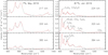 |
Fig. 1 Example of CIRS limb spectra acquired at 1°N in July 2016 (left panel, black line) and 81°S in January 2016 (right panel, black line) at three different tangent heights. They are compared with the best fit spectra (in red). These spectra can be compared with those of Fig. 1 of Mathé et al. (2020, their Figs. 1 and2) acquired at similar location, altitude, and date at higher spectral resolution. The band centered at 630 cm−1 includes C4H2 and CH3C2H emission; the band centered at 673 cm−1 includes HC3N, CO2, and C6H6. HCN, C2H2, and C3H8 emission bands are centered respectively at 713, 730, and 748 cm−1. C2H6, C2H4, and CH4 bands are centered at 815, 950, and 1300 cm−1, respectively. An overlap between FP3 and FP4 spectra occurs in the 1000–1050 cm−1 spectral range. |
4.1.1 High-southern latitudes
The most striking seasonal changes in temperature between Ls = 66° and Ls = 93° were observed in the southern hemisphere at latitudes higher than 30°S, where the stratopause altitude varied with latitude in a complex way. The southern polar stratopause reached its highest temperature close to the south pole (Figs. 2 and C.1), its temperature increased by 10 K from March to September 2015 (Ls = 66°−72°) and by 22 K from May 2016 to February 2017 (Ls = 78°−87°) to reach its highest value of 207 K. For the time period studied here, the altitude of the stratopause was globally decreasing towards mid-latitudes.
At deeper levels, the polar stratosphere was at its coldest in March and September 2015 (Ls = 66° and Ls = 72°) with temperatures lower than 120 K observed below the 0.06 mbar pressure level (260 km altitude) in March and the 0.2 mbar level (~200 km) in September. As the southern autumn was progressing, these low temperatures were observed to propagate deeper.
4.1.2 Mid-southern latitudes
Interestingly, the 30°S latitude seemed to be a transition in the structure of the thermal field from September 2015 (Ls = 72°) to May 2016 (Ls = 78°): on the low-latitude side, the stratopause was located deeper (~0.2 mbar, 250 km) than toward higher latitudes (at 40°S, it was located at 3 × 10⁻³ mbar, 450 km). It resulted in a double 173 K stratopause structure at 30°S (Figs. 2 and C.1). On both sides of 30°S, the stratopause remained at similar pressure levels until May 2016, while in February 2017 the two local temperature maxima seemed to have merged into a single one around 3 × 10⁻² mbar (340 km). This new structure was observed until the southern winter solstice in May 2017, the last date for which we have limb observations at this latitude.
4.1.3 Northern hemisphere
Thermal profiles in the northern hemisphere showed moderate changes during the second half of the northern spring. Altitude of the stratopause remained the same (~300 km, 0.1 mbar) at all latitudes from Ls = 67° to Ls = 93° (May 2015 to September 2017) with similar temperature (about 175–180 K) everywhere except at latitudes higher than 70°N, where the stratopause was typically 5 K warmer than at lower latitudes. After the northern summer solstice (for Ls = 93°), at high-northern latitudes the stratospherewas ~2 K colder and the stratopause 5 K colder than at Ls = 76° (February 2016), while an opposite trend was observed in the mesosphere, which was ~5 K warmer (in the 0.2−1 × 10⁻² mbar region) afterthe northern summer solstice than earlier in the spring.
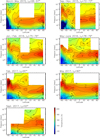 |
Fig. 2 Temperature meridional cross sections from March 2015 to September 2017. Contours are given every 5 K from 110 to 205 K; the color scale is the same for all plots. In the equatorial region, pressures of 1, 0.1, 0.01, 10−3, and 10−4 mbar roughly correspond to altitudes of 200, 300, 400, 500, and 600 km, respectively. Regions without information are represented in white; they correspond to missing data or pressure levels not probed by nadir observations. Red ticks on the x-axis give latitudes of observations used to retrieved the global map. |
4.1.4 Possible correlation between mesospheric temperature and insolation
We infer a local temperature maximum in the mesosphere around 500 km (10−3 mbar) during Titan’s daytime. For instance, a 165 K temperature local maximum was observed at this pressure level at high-northern latitudes in May 2015, at a solar zenith angle (SZA) of 63–90°, and February 2016 (17:00 local time, SZA = 60–66°), at mid-northern latitudes and the equator in June 2016 (~15:00 local time, SZA = 30–60°), and around the equator and at low-southern latitudes in February 2017 (12:30 local time, SZA = 19–45°). In contrast, it seems that the coldest mesospheric temperatures were observed during the night; for instance, temperatures about 5 K higher were found at the end of the day above 10−3 mbar at mid-northern latitudes in November 2015 (local time ~17:50, SZA = 68–85°) than in the middle of the night in May 2015 (local time ~01:30, SZA of 95–113°). In the southern hemisphere the lowest mesospheric temperatures were also observed during the night; for instance, in February 2017, the 10−4-mbar level temperature was found to increase from 162 K at 09:22 local time at 50°S (SZA = 82°) to 167 K at 12:48 at 2°N (SZA = 26°).
In the northern hemisphere, which was experiencing spring, we also inferred that the more illuminated high-northern latitudes showed higher mesospheric temperatures. For instance, in September 2017 the mid-northern latitude mesosphere (from Equator to 40°N, SZA = 106−153°, 21:30-22:47 local time) was ~5 K colder at 10−4 mbar than the constantly insolated high-northern latitude (local time ~20:30, SZA = 72–85°). A similar mesospheric temperature trend was also observed in May 2015 as the colder mid-northern latitude mesosphere was in the night (~01:30 local time, SZA = 90-113°) and the high-northern latitude mesosphere was insolated (SZA = 60-86°).
Mesospheric temperatures seem to be correlated with solar insolation even if adiabatic heating (respectively cooling) due to air subsidence (respectively upwelling) can also impact the mesospheric temperatures. This possible correlation, which can only be detectable in the mesosphere where the radiative time constant is about a few Titan hours (Bézard et al. 2018), was not observed deeper at the stratopause and stratospheric levels, consistently with the predicted radiative time constant greater than one Titan day there (Bézard et al. 2018).
4.2 Molecular gas mixing ratio meridional cross sections
Outside the southern polar region C2H2, HCN (Figs. 3, A.2, and C.1 middle and bottom panel) and C2H6 (Figs. A.1 and C.2 bottom panel) are the molecules whose VMR could be derived up to a few 10−4 mbar (500-600 km). C4H2 and CH3C2H VMR (Figs. A.3, A.4 and C.2) were generally determined up to a few 10−3 mbar (450–500 km). C3H8 and C2H4 mixing ratios (Figs. A.5, A.8, C.3 and C.4) were usually inferred up to 10−2–10−3 mbar (400–450 km) and HC3N and C6H6 (Figs. A.6, A.7, and C.3) were mostly detected at high latitudes up to 600 km at the south pole, while in the mid- and low-latitude regions, their VMRs (usually lower than 10−9) should be considered as upper limits. Retrieved mixing ratio profiles including their error bars are available in the supplementary material and will be posted on the Virtual European Solar and Planetary Access (VESPA) portal2. Determination of the error bars follows the methodology described by Vinatier et al. (2010a). They include the uncertainty on the retrieved thermal profiles, the ± 2 km uncertainty on the vertical shift, and the spectral noise, all summed quadratically at each pressure level.
Before looking in detail at the spatial distributions of each molecule, we first depict the main common global spatial and temporal trends of the inferred VMR:
Most molecules were strongly enriched at high-southern latitudes inside the polar vortex because of the subsidence of the global circulation cell that settled in 2012 (Teanby et al. 2012; Vinatier et al. 2015) and transported enriched air from higher levels toward the deep stratosphere. Additionally, this polar air was isolated from the air at mid-southern latitudes by strong zonal winds (Achterberg et al. 2011, 2018; West et al. 2016) forming the polar vortex (see also Sect. 5.5). At a given date, all polar VMR distributions (except those of C2H6 and C3H8 that have limited vertical gradients and therefore show limited enhancement by subsidence) showed very steep meridional gradients at high-southern latitudes, tracing the polar vortex barrier (Teanby et al. 2008). Depending on the molecules, polar enhancements were the greatest in 2015 and in January 2016. In March 2015 the molecules showing the steepest concentration meridional gradients across the polar vortex boundary were C2H4, C3H4, C6H6, HC3N, and HCN, which varied from a factor of 10 for HCN to three orders of magnitude for HC3N and C6H6. In September 2015, this polar enriched region had a wider latitudinal extension than in March 2015 and January 2016, and displayed stronger enrichments than in May 2017, suggesting changes in the horizontal structure of the polar vortex over this period.
In May 2017, at high-southern latitudes (between 30°S and 60°S) and at altitudes higher than 500 km (10−3 mbar), C2H2, C2H6, C4H2, CH3C2H, and HCN were more abundant than earlier in the season, while their polar enhancements in the 10−1–10−3 mbar region were less pronounced, suggesting some changes in the global circulation occurring close to the southern winter solstice.
In the deep stratosphere, typically below the 1 mbar level, at mid- and low latitudes all molecular VMRs (except for C2H4 which does not condense) decreased with depth as the main sink of these molecules is condensation, usually occurring below the 10 mbar level (~100 km). Some molecules, like HCN, C4H2, and CH3C2H, show steep slopes in the contours of constant mixing ratio at low- or mid-latitudes (see, e.g., Fig. A.4 in May-June 2016 or Fig. A.2 in Sept.-Nov. 2015), which suggests that upwelling was transporting deeper air (depleted due to condensation) to upper levels in the stratosphere.
Mesospheric depletions in C2H2, HCN, and C2H6 (Figs. 3, A.1, A.2, C.1 and C.2), which are the molecules for which we can derive information at the highest levels, have been observed since September-November 2015 (Ls = 72−73°). This depletion seems to have been initiated at high-northern latitudes in May 2015 (Ls = 67°) and has extended down to mid-southern latitudes in September 2015 (Ls = 72°).
Although at high-northern latitudes the upwelling branch of the global circulation cell has been in place since probably mid-2011 (Vinatier et al. 2015), a region located at latitudes higher than 60°N and altitudes between 200 and 300 km (Figs. 3 to 4 and Figs. C.1 to C.4) remained enriched in photochemical compounds (including haze) until the northern summer solstice, with a tendency to vanish after this date. Most of these molecular enrichments were located at the stratopause level. This suggests that the stratopause could be a sort of stagnancy region with limited mixing or that the northern winter residual circulation cell (which keeps some of the winter polar enriched air in the deep stratosphere up to the stratopause) was still present over the entire spring, as predictedby the IPSL Titan GCM, albeit limited to the deep stratosphere for all compounds (see Sect. 5.6).
In the following subsections we detail some specific trends observed for groups of molecules showing similar spatial and temporal behavior.
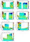 |
Fig. 3 C2H2 volume mixing ratio meridional cross sections from March 2015 to September 2017. Regions without information are represented in white; they correspond to missing data or pressure levels not probed by nadir observations. Red ticks on the x-axis give latitudes of observations used to retrieved the global map. |
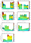 |
Fig. 4 Haze mass mixing ratio meridional cross sections from March 2015 to September 2017, determined from the haze extinction meridional cross sections displayed in Fig. A.9. Regions without information are represented in white; they correspond to missing data or pressure levels not probed by nadir observations. |
4.2.1 C2H2, HCN, C2H6, and C3H8 VMR meridional cross sections
The most abundant trace gases are C2H6, C2H2, HCN and C3H8. Their mixing ratios (with the exception of C3H8) can be derived at the highest altitudes from one pole to another (typically up to 10−3–10−4 mbar, 500–600 km).
The C2H6 and C3H8 VMRs (Figs. A.1, A.5, C.2 and C.3) show the less pronounced stratospheric vertical gradient of all the studied molecules. While C2H6 can be detected up to 550–650 km, C3H8 is usually determined up to 400 km (10−3–10−4 mbar). Both molecular VMRs varied at most by a factor of 5 in the whole stratosphere and showed a factor of 3 southern polar enhancement compared tomid-southern latitudes in the stratosphere and mesosphere. At high-northern latitudes, between 150 and 250 km (1–0.1 mbar), C3H8 remained enriched by a factor of 4 compared to latitudes lower than 60°N from 2015 to September 2017 and C2H6 remained enriched by a factor of 2 from 2015 to May 2017, before being depleted after the northern summer solstice.
In the northern mesosphere, above the 10−2 mbar level (400 km), between May and November 2015, we derived strong depletions of C2H2, HCN (both depleted by a factor of ~10 at 10−3 mbar, 500 km altitude, Figs. 3, A.2 and C.1), and C2H6 (depleted bya factor of ~2). This depletion was also observed at mid-southern latitudes at the same pressure level in September 2015, in 2016, and up to May 2017, while in September 2017 this depletion was only observed at latitudes higher than 50°N.
In May 2017, in the southern mesosphere, C2H2, HCN, and C2H6 were enriched above the 10−3 mbar level compared to earlier observations. Simultaneously, the southern polar stratosphere was less enriched in C2H2 and HCN than in 2015 and 2016, which suggests some global dynamical changes at high-southern latitudes near the southern winter solstice.
In the deep polar southern stratosphere, in 2015 and 2016, the combined low temperatures and high polar enhancements resulted in saturation of HCN occurring at unusually high altitudes: at 0.05 mbar (250 km) in March 2015 and 0.15 mbar (195 km) in September 2015. This is consistent with the detection of HCN ice in the VIMS spectra of the southern polar stratospheric cloud since mid-2012 (de Kok et al. 2014; Le Mouélic et al. 2018).
Interestingly, in 2015 and 2016 the cross section contours of constant HCN VMR at low latitudes in the deep stratosphere showed steeper slopes than those of C2H2, C2H6, and C3H8; these three VMRs were more or less constant at a given pressure level for all the dates studied here. As the HCN VMR vertical gradient is steeper than those of C2H2, C2H6, and C3H8, vertical dynamical transport has a larger impact on the HCN VMR profile. The overall shape of the HCN VMR contours at mid- and low latitudes suggests stratospheric upwelling of air at mid- and low latitudes in 2015 and 2016.
4.2.2 C4H2 and CH3C2H VMR meridional cross sections
The molecules C4H2 and CH3C2H (Figs. A.3, A.4, and C.2) show quite comparable stratospheric and mesospheric VMRs, even though CH3C2H was typically ~3 times more abundant than C4H2 above the 0.5 mbar level, and the C4H2 VMR vertical gradient is steeper than that of CH3C2H in the deep stratosphere, between 1 and 5 mbar.
Like other molecules, C4H2 and CH3C2H were strongly enriched in the southern polar region compared with lower southern latitudes. For instance, in March 2015 at the 0.1 mbar level (~250 km) the C4H2 VMR increased from 10−8 at 69°S to 7 × 10⁻⁷ at 84°S and CH3C2H varyied from 2 × 10⁻⁸ to 2 × 10⁻⁶ in the same latitude range. In the mesosphere, at 10−3 mbar, within the same latitude range, both molecules showed enhancement of a factor of 10 in 2015 and in January 2016, and a factor of 5 in May 2017. These enhancements were comparable to those observed for C2H2 and HCN atthe same pressure level in the same period.
At high-northern latitudes, both molecules were locally enriched by a factor of 7 to 9 in a limited zone comprised between 1 and 0.1 mbar and from 50°N to the pole. In September 2017, after the northern summer solstice, this enriched region seemed to have disappeared for C4H2 and was still observed for CH3C2H. In contrast to C2H2 and HCN, which showed a depleted layer at pressures lower than 10−2 mbar (as previously discussed), C4H2 and CH3C2H showed enhancements in this region.
4.2.3 C2H4, C6H6, HC3N VMR meridional cross sections
C2H4, HC3N, and C6H6 (Figs. A.6, A.7, A.8, C.3, and C.4) are the molecules that showed the strongest meridional enhancements at high-southern latitudes from 2015 to 2017. For instance, in the 10−2–10−3 mbar range these molecules were enriched between 70°S and 84°S by factors of 130, 100, and 40, respectively, with respect to latitudes lower than 65°S. HC3N and C6H6 were strongly depleted at altitudes lower than 250 km (0.1 mbar) likely due to their condensation. Because of their steep VMR meridional gradient near the south pole, these molecules can be regarded as the best tracers of the polar vortex boundary. In 2015, their VMR cross sections were compatible with a vortex boundary that was more confined toward the south pole between 300 and 400 km than at higher and lower altitudes. This gave it an anvil shape for the enriched zone on the maps of Figs. C.3, C.4, with a “tongue” of enriched air extending below 250 km toward lower latitudes. At 1 mbar (Figs. A.6–A.8) this tongue would correspond to a photochemical compound enriched torus enshrouding the polar region and its stratospheric polar cloud. We note that the tongue is also observed for CH3C2H (Figs. A.4 and C.2), C4H2 (A.3 and C.2), HCN (A.2 and C.1), and C2H2 (3 and C.1). In September 2015, using the boundary shape of the polar enriched zone we can deduce that the polar vortex was less confined around the south pole and that its boundary seemed to have extended down to almost 60°S around 300 km. At this date, and in January 2016, the meridional VMR gradients of C2H4, C6H6, and HC3N were less steep than in March 2015 and their enhancements extended down to 30°S at high altitude (higher than 300 km). While later (in May 2017) the same high-altitude VMR values were observed beyond 60°S. This suggests that the polar vortex was at its tightest latitudinal confinement in March 2015, then extended between March and September 2015, and retracted again in early 2016. This evolution is similar to the variation of the horizontal extension of the southern polar cloud observed by Cassini/VIMS in the same period (see Le Mouélic et al. 2018, their Fig. 4).
In the northern hemisphere, at latitudes higher than 60°N and in the 150–300 km altitude range, these molecules were enriched by factors of 10 to 100 compared to neighboring latitudes and altitudes. In March 2015 HC3N seemed to present a second enriched zone above 350 km. The C2H4 VMR showed the most complex vertical profile at high-northern latitudes with several enriched zones, one in the 250–300 km range and another below 150 km observed in March 2015 and February 2016, while some enrichment was also observed in September 2015 at altitudes higher than 400 km.
4.2.4 Haze mass mixing ratio meridional cross sections
We determined the haze mass mixing ratio from the retrieved haze optical depth assuming aerosol composed of 3000 monomers of 0.05 μm radius each (Tomasko et al. 2008) with a bulk density of 0.6 g cm−3. Haze mass mixing ratio cross sections determined from the 600–620 cm−1 continuum thermal emission (FP3 spectra) are displayed in Figs. 4 and C.4 (middle). They are also compared in Fig. C.4 with the haze mass mixing ratio determined from the 1000–1100 cm−1 range acquired by the FP4. Uncertainties on the continuum at very low radiance levels are responsible for the differences in the meridional cross sections inferred from both focal planes. The haze spatial distribution displays similarities with those of the trace gases; it is strongly enriched in the southern polar vortex (by at least a factor of 10 at 400 km, 10−2 mbar) compared to mid-southern latitudes.
At high-northern latitudes the haze is also enriched in a confined region beyond 50°N and between 1 and 0.1 mbar (200–300 km), like most of the molecules studied here. Like C2H2, HCN, and C2H6, the haze mass mixing ratio is depleted in the northern mesosphere in November 2015, June 2016, and also probably in February 2017, while the mesosphere in May 2015 and September 2017 was enriched in haze. In September 2017, an enriched haze layer was inferred at 10−2 mbar (400 km) between 20°N and 60°N. This last observation is compatible with the ISS observation of a haze layer at ~400 km between 25°N and 50°N at the same date (Seignovert et al. 2020).
The haze mass mixing ratio profile globally increases with height because aerosols are produced in the upper atmosphere and are removed by sedimentation. Interestingly, in March and September 2015, we inferred a depletion in haze in the southern polar region below the 0.1 mbar level, where C6H6, HC3N, and HCN were condensing. This suggests that haze is efficiently removed in this region, probably because aerosols serve as condensation seeds for condensing molecules.
4.3 Summary
In summary, in the second part of the southern fall, all photochemical compounds were enriched at the south pole by the subsiding branch of the global circulation cell. By assuming that this enriched air was confined at high-southern latitudes by the polar vortex, the changes in the meridional cross sections of the VMR can be seen as tracers of the horizontal and vertical changing structure of the southern polar vortex. Photochemical species high enhancements combined with the unusually low polar temperatures observed in the deep stratosphere resulted in condensation between 0.1 and 0.03 mbar (240–280 km) of HCN, HC3N, C6H6, and possibly C4H2 in March 2015 (Ls = 66°). These molecules were observed to condense progressively deeper from the south pole. Right outside this condensation zone, the subsidence transported the enriched air toward the mid-latitude deep stratosphere probably forming a torus of enriched air enshrouding the polar vortex at 200 km and below.
At high-northern latitudes, stratospheric enrichments rema- ining from the previous winter were observed below 300 km between 2015 and May 2017 (Ls = 90°) for all chemical compounds, and up to September 2017 (Ls = 93°) for C2H2, C2H4, CH3C2H, C3H8, and C4H2. These enrichments were observed at different altitudes depending on the molecule. It was observed at 0.1–0.5 mbar (250–300 km) for the haze, C2H2, C2H4 (with a more complex vertical structure for C2H4), CH3C2H, C4H2, and HCN. This pressure region approximately corresponds to the location of the stratopause. In 2015 and 2016, the corresponding C3H8 enrichment zone was observed slightly deeper, in the 0.3–1 mbar pressure range (150–250 km), and even deeper for HC3N, which was enriched in the 0.5–2 mbar range. C6H6 was also enriched, but only deeper than the 1 mbar level. In September 2017 these local enhancements were less pronounced than earlier for C2H2, C4H2, CH3C2H, HC3N, and HCN, and no longer observed for C2H6 and C6H6, which suggests a change in the northern polar dynamics near the summer solstice.
In the mesosphere, C2H2, HCN, and C2H6 were depleted from the north pole to the mid-southern latitudes, while C4H2, C3H4, C2H4, and HC3N seem to have been enriched in the same region. In the deep stratosphere, all molecules except C2H4 were depleted due to their condensation sink located deeper than 5 mbar outside the southern polar vortex. The HCN, C4H2, and CH3C2H VMR cross section contours showed steep slopes near mid-latitudes or close to the equator, which can be explained by upwelling air in this region. Upwelling is also supported by the C2H4 enriched air observed in the northern hemisphere.
5 Discussion
5.1 Thermal field
In the deep stratosphere, our results can be compared with those of Teanby et al. (2019), who inferred the temperature seasonal evolution from CIRS nadir spectra acquired at a spectral resolution of 3 cm−1. The temperatures derived in our study at 0.1, 1, and 5 mbar are overall very consistent with their results from 2015 to 2016. A comparison of our thermal field at 5 mbar with results from Sylvestre et al. (2020), who derived temperatureat 6 mbar from far-infrared thermal emission acquired by CIRS (using focal plane 1), also shows good consistency.
In our previous study focusing on Titan’s early spring from July 2009 to May 2013 (Vinatier et al. 2015), we were able to infer the pole-to-pole thermal field from December 2009 to February 2012. We recall that from 2012 to 2015 the Cassini orbit inclination prevented us from probing Titan’s polar limbs. The derived thermal field in March 2015 differs greatly from that in 2012 mostly at polar latitudes. The strongest seasonal changes occurred at high-southern latitudes, where a 30 K decrease was derived between 2012 and 2015 in the deep stratosphere together with a 15 K increase at 2 × 10⁻³ mbar. The seasonal evolution of the thermal field at high-southern latitudes results from a complex interplay between adiabatic heating from the descending branch of the circulation cell and enhanced radiative cooling from the enriched molecules, as detailed by Teanby et al. (2017). In 2015, the southern polar vortex was already well established.
The high-northern latitude stratopause was observed about one pressure decade deeper in 2015 than in 2012 and was 5 K warmer. The deeper location of the stratopause at high-northern latitudes could be explained by the combined effect of adiabatic cooling at the 10−2–10−3 mbar pressure range by the upwelling branch of the global circulation, and the increasing mid-spring insolation.
The mid- and low-latitude stratopause was located at the same pressure in 2012 (Vinatier et al. 2015) and 2015, but the 10–20°N stratopause was 2K colder in 2015 than in 2012 at 0.2–0.3 mbar, which may result from Saturn’s orbit eccentricity (Bézard et al. 2018).
The temperature profiles we derived can be compared with those of Mathé et al. (2020) inferred from CIRS limb spectra acquired at 0.5-cm−1 spectral resolution at comparable latitudes and time. Their dataset probed the same pressure region as ours. The agreement with their mid-northern and high-northern latitude profiles in 2015 and 2016 is very good. Our derived temperatures are also consistent below the mesosphere with their equatorial and mid-southern latitude profiles. However, we derived mesospheric temperatures that were higher by ~5–10 K than their 2017 equatorial values and their 2016–2017 mid-southern values. At the south pole, our thermal profiles are also in very good agreement with theirs at similar latitudes and longitudes. For instance, in March 2015 Fig. C.1 shows that the thermal field is not symmetrical around the south pole with the thermal profile at 81°S 255°W (17:58 local time, right-hand side of the pole in Fig. C.1) showing a stratopause (at 400 km) 12 K warmer than at 78°S 119°W (02:52 local time, left-hand side of the pole in Fig. C.1). As this later thermal profile is in agreement with that inferred by Vinatier et al. (2018) and with the results of Mathé et al. (2020) in the 10−2–10−4 mbar range, which were extracted from other CIRS limb data acquired at the same date, longitude, and 15 h apart, it strengthens our derived asymmetry of the thermal field around the south pole in March 2015. This asymmetry probably results from the different insolation conditions between these two limb observations.
5.2 Molecular gas mixing ratio meridional cross sections
Our VMR profiles can be compared with the retrieved profiles of Mathé et al. (2020), who used CIRS limb spectra acquired at 0.5 cm−1 over the entire Cassini mission. Our retrieved VMR profiles are overall in very good agreement with their results. For instance, at high-northern latitude, they also inferred similar local VMR maxima for C2H2 and HCN in the 0.1–1 mbar pressure range, they derived a local VMR minimum at ~0.005 mbar with equivalent VMR values. Other VMR profiles that we derived in this study are also consistent with their results, except at 81°S–125°W in March 2015 as they retrieved C2H2 and HCN VMR 10 times higher than ours at and above 10−4 mbar, while our profiles agree deeper than this pressure level for C2H2. However, at this location, other molecular VMRs are consistent within the error bars. These observations have larger uncertainties than any other because of the low temperature there, which can explain discrepancies between the two studies.
The mixing ratios we retrieved around 1 mbar can be compared with those retrieved by Teanby et al. (2019) and Coustenis et al. (2020), who inferred VMRs from CIRS nadir spectra acquired at 2.5 and 0.5 cm−1 spectral resolution, respectively. Common molecules between our study and Teanby et al. (2019) are C2H2, C2H4, C2H6, CH3C2H, C4H2, HCN, and HC3N; Coustenis et al. (2020) additionally retrieved VMR of C3H8 and C6H6. As vertical information is very limited from nadir observations, both studies assumed constant-with-height mixing ratio profiles above the condensation level, which makes a detailed comparison partially meaningful as our derived profiles show strong vertical variations with altitude. Nevertheless, around 1 mbar the relative decrease in molecular VMRs at the north pole and their relative increase at the south pole (Teanby et al. 2019) in the 2015–2017 period in is overall agreement with our results. However, because of their constant-with-height VMR assumption, these authors could not derive the local enhancement that we inferred at high-northern latitude in the 1–0.1 mbar pressure range. In general, our stratospheric (in the 5–0.5 mbar range) inferred VMR are in good agreement with those derived by Coustenis et al. (2020).
We derived the highest VMR in the south pole mesosphere in March 2015, when the polar vortex was at its tightest latitudinal confinement. Our derived VMRs of C2H2, HCN, CH3C2H, and C4H2 inside the polar vortex at 600 km (2 × 10⁻⁵ mbar) are similar to the VMRs measured in situ by the Cassini Ion Neutral Mass Spectrometer (INMS) above 1000 km (Vuitton et al. 2007; Cui et al. 2009; Magee et al. 2009). This observation, also reported by Mathé et al. (2020), suggests that subsidence at the south pole transports enriched air from altitudes much higher than 600 km. Additionally, the derived thermal zonal wind (see Sect. 5.5) also supports a more confined polar vortex in March 2015 with winds of ~240 m s−1 reaching at least 600 km, with subsidence therefore necessarily coming from higher altitudes.
The only molecule among all those studied here that does not condense in Titan’s atmosphere is C2H4. This explains why it is enriched in the deep stratosphere by advection from the fall–winter polar region towards the spring–summer pole in the deep atmosphere by the deep branch of the global circulation (Vatant d’Ollone 2020). Additionally, C2H4 is photodissociated below 500 km and reacts with H atoms to form C2H5 (Vuitton et al. 2019), which can explain its depletion at mid- and low latitudes above 150 km. The global northern hemisphere enrichment compared to the southern hemisphere below 300 km observed since November 2015 (Ls = 73°) could be explained by a global vertical transport of this molecule at mid- and high-northern latitudes, which is compatible with the spring and summer ascending branch predicted by GCMs (e.g., Vatant d’Ollone 2020). The complex northern polar structure of its VMR meridional cross section suggests a complex circulation pattern, perhaps including two small circulation cells that could have coexisted in 2015 and 2016, keeping the C2H4 enrichments in two distinct altitude ranges (one around 0.1 mbar and another one deeper than 1 mbar).
5.3 Local mesospheric minimum VMR of C2H2, C2H6, and HCN
According to Vuitton et al. (2019), the predicted lifetimes of C2H2, C2H6, and HCN in the mesosphere are mostly controlled by vertical transport timescales, resulting in lifetimes of 14 Titan days (230 days) at 500 km (~10−3 mbar) for C2H2, 100 Titan days for C2H6, and 1000 Titan days for HCN. Chemical lifetimes decrease with altitude, and it is possible that the observed mesospheric depleted air comes from higher levels where these molecules are more efficiently photodissociated. Assuming that the C2H2- and HCN-depleted air observed at 80°N on May 9, 2015, was horizontally advected to 40°S on September 29, 2015, would imply an horizontal advection of 50 cm s−1, a value higher but not so far from the 0.1–0.2 m s−1 predicted by the IPSL Titan GCM in diurnal average (Vatant d’Ollone 2020; Vatant d’Ollone et al. 2018). Using the continuity equation, this horizontal velocity would imply a subsidence vertical velocity of ~3 mm s−1 inside the southern polar vortex at 10−2 mbar (~400 km), which is consistent with estimations of Teanby et al. (2017) in 2015 using a radiative model and from their derived mixing ratio profiles. Another possibility to explain the presence of this depleted zone could be diurnal effects, which is at odds with the conclusion of Vuitton et al. (2019). We observe a correlation between the mesospheric temperature maximum observed during the day (displayed in yellow and orange in Figs. 2 and C.1) and the lower VMRs of C2H2, C2H6, and HCN. Instead, during the nighttime the mesospheric VMRs seemed to be enhanced. This hypothesis needs other data analysis to be confirmed or refuted.
5.4 Haze extinction meridional cross sections: comparison with ISS observations
Seignovert et al. (2020) derived the seasonal variation of Titan’s haze extinction from October 2004 to September 2017 in the 350–550 km altitude range from the analysis of the Cassini Image Sub-System Narrow Angle Camera in the CL1-UV3 UV filter at 338 nm. We can compare the spatial distribution of extinction we derived from CIRS in the 350–450 km range, which is generally the overlap altitude range probed by UV and thermal infrared observations. Seignovert et al. (2020) inferred complex temporal variation of the haze extinction in the stratopause and mesospheric levels with high temporal variability. In order to compare haze extinction coefficients derived from CIRS observations at 1090 cm−1 and the UVIS ones at 338 nm (29 586 cm−1), we applied a multiplicative factor equal to 1.22 × 10⁻³ derived from the far-IR to UV spectral dependence of the aerosol cross sections of Vinatier et al. (2012, see Fig. 2 therein). A comparison of our haze extinction coefficient maps with those derived from ISS observations acquired at similar dates is displayed in Appendix D. In the overlapping altitude range, agreement is overall within a factor of 2, which is typically the uncertainty on the haze extinction coefficient derived from CIRS limb spectra above 350 km. The largest difference is inferred in September 2017, which corresponds to an ISS observation with a limited latitudinal coverage for which Titan’s center adjustment, and therefore the altitude grid extraction, is not as well constrained as for other ISS datasets (see Seignovert et al. 2020).
5.5 Thermal winds
Performing a scale analysis for Titan’s parameters of the different terms of the momentum equation in spherical coordinates projected over the northward direction gives the remaining terms:
![Mathematical equation: \[ 2 \Omega {\textrm{sin}}(\phi) u + \frac{\textrm{tan}(\phi)}{r} u^{2} + \frac{1}{\rho r} \frac{\partial p}{\partial \phi}\Bigg|_z\,{=}\,0. \]](/articles/aa/full_html/2020/09/aa38411-20/aa38411-20-eq1.png)
Here u is the zonal wind velocity (eastward), Ω the rotation rate of Titan, r the sum of Titan’s radius and altitude, ϕ the latitude, p the pressure, and ρ the atmospheric number density. Frictional forces can be neglected in the stratosphere. Appendix E gives solutions of this equation that we applied to calculate u from the meridional pressure gradient. Titan’s zonal winds were previously determined from the thermal field derived from CIRS limb and nadir observations by Flasar et al. (2005) and Achterberg et al. (2008) during Titan’s northern winter, by Achterberg et al. (2011) from winter to northern spring, and extended by Achterberg et al. (2018) over early northern summer but deeper than 0.05 mbar as they used CIRS nadir datasets. Our zonal wind integration differs from these previous studies as we did not integrate the thermal wind equation over cylinders concentric around Titan’s rotation axis (Flasar et al. 2005), but instead performed integration in spherical coordinates (see Appendix E). We set the zonal wind at 5 mbar to 120 m s−1, which is compatible with in situ measurements acquired by the Doppler Wind Experiment aboard Huygens during the probe descent (Bird et al. 2005; Folkner et al. 2006).
Figure 5 shows the meridional cross sections of zonal wind velocity (eastward) derived from the thermal fields displayed in Fig. 2. During the studied period all the derived meridional cross sections of zonal wind show a clear asymmetry between the northern and southern hemispheres with zonal winds much faster in the southern hemisphere than in the northern one. If we consider that the southern polar vortex boundary is characterized by the strongest zonal winds around the south pole (circumpolar jet reaching 240–280 m s−1), our derived zonal wind maps in March 2015 and September 2015 show that the polar vortex was confined to latitudes higher than 70°S in March and 60°S in September. This horizontal extension is consistent with results from the VMR cross sections that display the same latitudinal extension of the enriched zone between the two dates (see, e.g., Fig. A.2). In 2016 the high-southern latitude jet seemed to slow down while migrating toward low-southern latitudes in June 2016 and February 2017. A less pronounced zonal wind local maximum was derived at 65°S at ~10−2 mbar in June 2016 and February and May 2017. Such temporal evolution of zonal winds can explain the temporal change in the VMR enrichment patterns at high-southern latitude described in Sect. 4.2, confirming that they are linked to the polar vortex changing structure.
In all of our derived stratospheric wind maps, the northern zonal winds are much weaker than the southern hemisphere winds with values typically lower than 160 m s−1, which is (given the studied period) totally consistent with momentum conservation in a superrotating atmosphere overturning cell leading to faster winds during autumn and winter in altitude. The northern wind speeds seemed to be globally higher in the deep stratosphere (deeper than 10−1 mbar) than above the stratopause (above 10−1 mbar). This last point, added to the fact mentioned previously that the stratopause seems to be an area of limited mixing for some species, supports the idea (supported by models such as the ISPL Titan GCM) that the stratopause could act as a separation between stratospheric and mesospheric circulation pattern (Vatant d’Ollone 2020; Vatant d’Ollone et al. 2018).
We can compare our derived zonal wind cross section with the one derived by Achterberg et al. (2018) in 2016 and 2017. Their maps are determined below the 0.05 mbar level because they were calculated from thermal fields inferred from CIRS nadir observations. Below this pressure range, our derived zonal wind horizontal and vertical structures are in good agreement.
Lellouch et al. (2019) determined zonal wind velocities in July and August 2016 from the Doppler shifts of submillimeter lines for several molecules acquired by ALMA (Atacama Large Submillimeter Array) interferometer. From all their studied molecules, which probe different levels in the atmosphere, they derived wind maps with faster zonal winds in the southern hemisphere than in the northern hemisphere, along with an equatorial jet. Our derived thermal wind structures in May 2016 are overall in very good agreement with their measurements as we derive wind values at 20°S (240–260 m s−1 in the 300–600 km range, or in the 0.1–10−4 mbar pressure range) comparable to their fitted values assuming solid-body rotation (210 m s−1 between 200 and 400 km, and 260–290 m s−1 between 400 and 700 km). Our larger zonal wind observed at low-southern latitudes in May 2016 (and probably also in February and May 2017) is consistent with the Lellouch et al. (2019) direct detection of an equatorial jet in August 2016. It should be noted, however, that for latitudes lower than 20° the  term in the zonal wind solution (see Appendix E) can amplify uncertainties on our derived wind profiles.
Our results show that two years before the southern winter solstice, the southern polar vortex structure was changing within a few Titan days, resulting in more or less pronounced molecular enhancements inside the polar vortex. One year before the summer solstice, two jets are derived in the southern stratosphere near 70°S and at mid-southern latitudes.
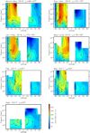 |
Fig. 5 Zonal wind cross sections from March 2015 to September 2017. Contours are given every 20 m s−1 ; the color scale is the same for all plots. Regions without information are represented in white. They correspond to missing data, pressure levels not probed by nadir observations, or regions not used to perform the wind calculation at low latitudes. |
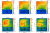 |
Fig. 6 Predictions of the IPSL Titan GCM for HCN volume mixing ratio (top) and the zonal wind (m s−1, bottom) for Ls = 68, 76, and 89°. Meridional circulation is superimposed with stream functions (109 kg s−1) in solid lines for clockwise circulation and dotted lines for counterclockwise. |
5.6 Comparison with the Institut Pierre Simon Laplace Titan Global Climate Model
Our VMR meridional cross sections can be compared with the predictions of the IPSL Titan GCM. This GCM, which has been recently upgraded to take into account coupling between chemistry, radiative transfer, haze microphysics, and global dynamics (Vatant d’Ollone 2020; Vatant d’Ollone et al. 2018), is currently the most complete. It models processes occurring in the middle atmosphere of Titan.
Figure 6 shows the predicted HCN VMR (top) and zonal wind (bottom) for Ls = 68°, 76°, and 89°, with corresponding stream functions for each season. At mid- and low latitudes, the molecular depletion that we observe in the deep stratosphere is predicted by the GCM to result from air ascending from condensation levels (see the predicted VMR in the 102–103 Pa region).
The northern winter residual circulation cell is predicted to extend from the north pole to ~50°N in the deep stratosphere and decrease in size with time, before vanishing around the northern summer solstice. Seasonal change of this residual circulation cell was responsible for the maintenance of the local northern polar stratospheric enhancements during spring. This result from the GCM, although predicted at deeper levels than observed here, could explain our local gas VMR and haze mass mixing ratio enrichment at the north pole deeper than 0.1 mbar, which slowly dissipated after the northern summer solstice. The IPSL Titan GCM also predicts that the southern mesosphere is more enriched in photochemical products than the northern mesosphere. This tendency is also observed here; however, we inferred southern enhancements that are more confined around the south pole than the GCM prediction before the southern summer solstice. This difference can be explained by the GCM top layer located at 10−1 Pa, which limits the vertical extension of the meridional circulation along with the horizontal resolution used in the model, which is too low to reproduce steep meridional gradients. Despite these limitations, the IPSL Titan GCM predicts a high-southern latitude mesosphere (above the 10 Pa level) that is more enriched than earlier in photochemical compounds near the summer solstice, combined with a light depletion of polar air deeper than 10 Pa. This prediction is also in agreement with our observations, even though observed in a lower pressure range.
As in most of the models, predicted zonal winds for northern spring and summer are faster in the southern hemisphere than is the northern. Structure of the southern polar vortex is predicted to change within the observing time studied here, with a global decrease in zonal wind speed with time and development of a double equatorial jet, a stratospheric and a mesospheric. This predicted complex seasonal variation of the zonal wind is in very good agreement with our thermal zonal wind calculation, albeit with a pressure decade difference, which is again likely due to the vertical extension of the IPSL Titan GCM. Our derived equatorial thermal winds are much faster than those predicted by this GCM, which can be explained by their predicted thermal contrasts that are less pronounced than those inferred from CIRS data. Further discussions can be found in Vatant d’Ollone et al. (2018).
Acknowledgements
This work was funded by the French Centre National d’Etudes Spatiales (CNES) and the Programme National de Planétologie (INSU). M.S. and N.A.T. acknowledge support from the UK Science and Technology Facilities Council (grant number ST/MOO7715/1).
Appendix A: Additional figures
Meridional cross sections of the volume mixing ratios of C2H6, HCN, C4H2, CH3CCH, C3H8, HC3N, C6H6, C2H4 and the haze extinction are displayed in Figs. A.1–A.9, respectively.
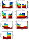 |
Fig. A.9 Haze extinction coefficient (given in cm−1 and representative of 1090 cm−1) meridional cross sections from March 2015 to September 2017. Extinction coefficient is derived from the fit of the 595–660 cm−1 spectral range and scaled to 1090 cm−1 using the spectral dependence derived by Vinatier et al. (2012). Regions without information are represented in white; they correspond to missing data or pressure levels not probed by nadir observations. |
Appendix B: Observations characteristics
Characteristics of the limb and nadir observations used in this study are listed in Tables B.1 and B.2, respectively.
Characteristics of the averaged FP4 limb spectra.
Characteristics of the averaged FP4 nadir spectra.
Appendix C: Altitude–latitude cross sections of the thermal field and photochemical species distribution
Figures C.1–C.4 give another way to display the thermal field (Fig. C.1) and the mixing ratios of trace gas distributions (Figs. C.1–C.4) with the altitude as vertical axis and on a polar projection with the north pole at the top and south pole at the bottom of each panel. This more compact visualization allows us to plot the distributions derived for all the studied dates in a single row. It is then possible to compare the spatial distributions of up to three molecules in a single figure. Color scales are the same as those in Figs. 2 to A.8. Additionally, Fig. C.4 displays a comparison of the haze mass mixing ratio distributions derived from the spectral continuum around 610 cm−1 (FP3, middle) and 1090 cm−1 (FP4, bottom). The main structures derived from the two spectral ranges are very similar except at altitudes higher than 400 km, where uncertainties on the continuum radiance become important.
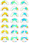 |
Fig. C.1 Thermal field (top), C2H2 (middle), and HCN (bottom) volume mixing ratio meridional cross sections from March 2015 to September 2017 (from left to right). |
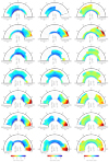 |
Fig. C.2 C4H2 (top), CH3C2H (middle), and C2H6 (bottom) volume mixing ratio meridional cross sections seasonal changes from March 2015 to September 2017 (from left to right). |
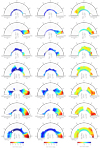 |
Fig. C.3 HC3N (top), C6H6 (middle), and C3H8 (bottom) volume mixing ratio meridional cross sections seasonal changes from March 2015 to September 2017 (from left to right). |
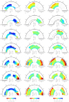 |
Fig. C.4 Meridional cross sections of C2H4 volume mixing ratio (top) and haze mass mixing ratio determined from the continuum in the spectral region around 610 cm−1 (FP3, middle) and 1090 cm−1 (FP4, bottom) from March 2015 to September 2017 (from left to right). |
Appendix D: Comparison of our derived meridional cross section of haze extinction with those derived from Cassini/ISS data
Figures D.1 and D.2 show the meridional cross sections of haze extinction derived in this study (left) compared to extinction inferred from Cassini ISS Narrow Angle camera observations at 338 nm (Seignovert et al. 2020).
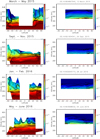 |
Fig. D.1 Comparison of the aerosol extinction coefficient at 1090 cm−1 derived from CIRS observations in 2015 and 2016 (left column) with those inferred from Cassini ISS Narrow Angle camera at 338 nm (right column) (Seignovert et al. 2020). Extinction is given in cm−1 and a factor 1.22 × 10⁻³ was applied to the extinction coefficient of Seignovert et al. (2020) in order to take into account the aerosol extinction spectral dependence between 338 nm and 1090 cm−1 (Vinatier et al. 2012). |
Appendix E: Integration of the thermal windshear equation
Integration of the thermal wind equation is performed over atmospheric parcels of altitude thickness δz, small compared to the pressure scale height (typically 40 km in Titan’s middle atmosphere) and over the latitude range δϕ. In the case of Titan a scale study of the projected momentum equations over a northward horizontal y-axis, with d y = (RT + z)dϕ = rdϕ, where RT is Titan’s radius, z and ϕ are the considered altitude and latitude, respectively, leading to the equation
 (E.1)
(E.1)
where u is the zonal wind velocity (eastward), Ω the rotation rate of Titan (4.56 × 10⁻⁶ rad s−1), z the altitude, ϕ the latitude, p the pressure, and ρ the atmospheric density. The frictional force component is neglected as it mostly has an impact inside the boundary layer. Deriving Eq. (E.1) with respect to z combined with the ideal gas law leads to
 (E.2)
(E.2)
where M is the mean molecular mass, T the temperature, and R the gas constant.
Integration of Eq. (E.2) over the jth layer of altitude range [zj, zj+1] yields
 (E.3)
(E.3)
with the solutions:
 (E.4)
(E.4)
with ![Mathematical equation: $C\,{=}\,\frac{1}{\textrm{tan}(\phi)}\frac{R}{M} \big[T_{j+1}(\phi)\frac{\partial {\textrm{ln}}(p_{j+1})}{\partial \phi} - T_{j}(\phi)\frac{\partial {\textrm{ln}}(p_{j})}{\partial \phi}\big ] - u_j^2 - 2\Omega {\textrm{cos}}(\phi) r_j u_j $](/articles/aa/full_html/2020/09/aa38411-20/aa38411-20-eq7.png) .
.
The plus sign (+) in the solution must be applied for eastward wind.
Because of the term  , which amplifies any errors on the pressure field (or temperature field) at low latitude, we only considered latitudes higher than 10°.
References
- Achterberg, R. K., Conrath, B. J., Gierasch, P. J., Flasar, F. M., & Nixon, C. A. 2008, Icarus, 194, 263 [NASA ADS] [CrossRef] [Google Scholar]
- Achterberg, R. K., Gierasch, P. J., Conrath, B. J., Michael Flasar, F., & Nixon, C. A. 2011, Icarus, 211, 686 [CrossRef] [Google Scholar]
- Achterberg, R. K., Gierasch, P. J., Nixon, C. A., & Flasar, F. M. 2018, in Cassini Science Symposium, 13th-17th August, Boulder, USA [Google Scholar]
- Anderson, C. M., Samuelson, R. E., & Nna-Mvondo, D. 2018, Space Sci. Rev., 214, 125 [CrossRef] [Google Scholar]
- Bézard, B., Vinatier, S., & Achterberg, R. K. 2018, Icarus, 302, 437 [CrossRef] [Google Scholar]
- Bird, M. K., Allison, M., Asmar, S. W., et al. 2005, Nature, 438, 800 [CrossRef] [Google Scholar]
- Coustenis, A., Achterberg, R. K., Conrath, B. J., et al. 2007, Icarus, 189, 35 [NASA ADS] [CrossRef] [Google Scholar]
- Coustenis, A., Jennings, D. E., Nixon, C. A., et al. 2010, Icarus, 207, 461 [NASA ADS] [CrossRef] [Google Scholar]
- Coustenis, A., Jennings, D. E., Achterberg, R. K., et al. 2020, Icarus, 344, 113413 [CrossRef] [Google Scholar]
- Cui, J., Yelle, R. V., Vuitton, V., et al. 2009, Icarus, 200, 581 [NASA ADS] [CrossRef] [Google Scholar]
- de Kok, R. J., Teanby, N. A., Maltagliati, L., Irwin, P. G. J., & Vinatier, S. 2014, Nature, 514, 65 [NASA ADS] [CrossRef] [Google Scholar]
- Feofilov, A., Rezac, L., Kutepov, A., et al. 2016, Titan Aeronomy and Climate, 2 [Google Scholar]
- Flasar, F. M., Kunde, V. G., Abbas, M. M., et al. 2004, Space Sci. Rev., 115, 169 [NASA ADS] [CrossRef] [Google Scholar]
- Flasar, F. M., Achterberg, R. K., Conrath, B. J., et al. 2005, Science, 308, 975 [NASA ADS] [CrossRef] [Google Scholar]
- Folkner, W. M., Asmar, S. W., Border, J. S., et al. 2006, J. Geophys. Res. Planets, 111, E07S02 [CrossRef] [Google Scholar]
- Jennings, D. E., Anderson, C. M., Samuelson, R. E., et al. 2012, ApJ, 761, L15 [CrossRef] [Google Scholar]
- Jennings, D. E., Achterberg, R. K., Cottini, V., et al. 2015, ApJ, 804, L34 [NASA ADS] [CrossRef] [Google Scholar]
- Jennings, D. E., Flasar, F. M., Kunde, V. G., et al. 2017, Appl. Opt., 56, 5274 [CrossRef] [Google Scholar]
- Kunde, V. G., Ade, P. A., Barney, R. D., et al. 1996, Proc. SPIE, 2803, 162 [NASA ADS] [CrossRef] [Google Scholar]
- Lebonnois, S., Burgalat, J., Rannou, P., & Charnay, B. 2012, Icarus, 218, 707 [NASA ADS] [CrossRef] [Google Scholar]
- Lebonnois, S., Flasar, F. M., Tokano, T., & Newman, C. E. 2014, The general circulation of Titan’s lower and middle atmosphere (Cambridge: Cambridge University Press), 122 [Google Scholar]
- Lellouch, E., Gurwell, M. A., Moreno, R., et al. 2019, Nat. Astron., 3, 614 [CrossRef] [Google Scholar]
- Le Mouélic, S., Rodriguez, S., Robidel, R., et al. 2018, Icarus, 311, 371 [CrossRef] [Google Scholar]
- Lora, J. M., Lunine, J. I., & Russell, J. L. 2015, Icarus, 250, 516 [CrossRef] [Google Scholar]
- Magee, B. A., Waite, J. H., Mandt, K. E., et al. 2009, Planet. Space Sci., 57, 1895 [NASA ADS] [CrossRef] [Google Scholar]
- Mathé, C., Vinatier, S., Bézard, B., et al. 2020, Icarus, 344, 113547 [CrossRef] [Google Scholar]
- Newman, C. E., Lee, C., Lian, Y., Richardson, M. I., & Toigo, A. D. 2011, Icarus, 213, 636 [CrossRef] [Google Scholar]
- Nixon, C. A., Ansty, T. M., Lombardo, N. A., et al. 2019, ApJS, 244, 14 [CrossRef] [Google Scholar]
- Seignovert, B., Rannou, P., West, R. A., & Vinatier, S. 2020, ApJ, submitted [Google Scholar]
- Sung, K., Toon, G. C., Mantz, A. W., & Smith, M. A. H. 2013, Icarus, 226, 1499 [CrossRef] [Google Scholar]
- Sylvestre, M., Teanby, N. A., Vinatier, S., Lebonnois, S., & Irwin, P. G. J. 2018, A&A, 609, A64 [CrossRef] [EDP Sciences] [Google Scholar]
- Sylvestre, M., Teanby, N. A., Vattant d’Ollone, J., et al. 2020, Icarus, 344, 113188 [CrossRef] [Google Scholar]
- Teanby, N. A., Irwin, P. G. J., de Kok, R., et al. 2007, Icarus, 186, 364 [CrossRef] [Google Scholar]
- Teanby, N. A., de Kok, R., Irwin, P. G. J., et al. 2008, J. Geophys. Res., 113, E12003 [CrossRef] [Google Scholar]
- Teanby, N. A., Irwin, P. G. J., Nixon, C. A., et al. 2012, Nature, 491, 732 [NASA ADS] [CrossRef] [Google Scholar]
- Teanby, N. A., Bézard, B., Vinatier, S., et al. 2017, Nat. Comm., 8, 1586 [CrossRef] [Google Scholar]
- Teanby, N. A., Sylvestre, M., Sharkey, J., et al. 2019, Geophys. Res. Letter, 46, 3079 [CrossRef] [Google Scholar]
- Tomasko, M. G., Doose, L., Engel, S., et al. 2008, Planet. Space Sci., 56, 669 [NASA ADS] [CrossRef] [Google Scholar]
- Vatant d’Ollone, J. 2020, PhD thesis, Sorbonne Université, Paris, France [Google Scholar]
- Vatant d’Ollone, J., Lebonnois, S., & Burgalat, J. 2018, European Planetary Science Congress (Berlin, Germany: TU Berlin), EPSC2018 [Google Scholar]
- Vinatier, S., Bézard, B., Fouchet, T., et al. 2007, Icarus, 188, 120 [NASA ADS] [CrossRef] [Google Scholar]
- Vinatier, S., Bézard, B., Nixon, C. A., et al. 2010a, Icarus, 205, 559 [NASA ADS] [CrossRef] [Google Scholar]
- Vinatier, S., Bézard, B., de Kok, R., et al. 2010b, Icarus, 210, 852 [CrossRef] [Google Scholar]
- Vinatier, S., Rannou, P., Anderson, C. M., et al. 2012, Icarus, 219, 5 [NASA ADS] [CrossRef] [Google Scholar]
- Vinatier, S., Bézard, B., Lebonnois, S., et al. 2015, Icarus, 250, 95 [NASA ADS] [CrossRef] [Google Scholar]
- Vinatier, S., Schmitt, B., Bézard, B., et al. 2018, Icarus, 310, 89 [CrossRef] [Google Scholar]
- Vuitton, V., Yelle, R. V., & McEwan, M. J. 2007, Icarus, 191, 722 [NASA ADS] [CrossRef] [Google Scholar]
- Vuitton, V., Yelle, R. V., Klippenstein, S. J., Hörst, S. M., & Lavvas, P. 2019, Icarus, 324, 120 [NASA ADS] [CrossRef] [Google Scholar]
- West, R. A., Del Genio, A. D., Barbara, J. M., et al. 2016, Icarus, 270, 399 [NASA ADS] [CrossRef] [Google Scholar]
Vertical profiles are accessible on the VESPA portal: (http://vespa.obspm.fr/planetary/data/). Fits of the observed spectra are available on request to S. Vinatier.
Vertical profiles are accessible on the VESPA portal: http://vespa.obspm.fr/planetary/data/). Fits of the observed spectra are available on demand to S. Vinatier.
All Tables
All Figures
|
Fig. 1 Example of CIRS limb spectra acquired at 1°N in July 2016 (left panel, black line) and 81°S in January 2016 (right panel, black line) at three different tangent heights. They are compared with the best fit spectra (in red). These spectra can be compared with those of Fig. 1 of Mathé et al. (2020, their Figs. 1 and2) acquired at similar location, altitude, and date at higher spectral resolution. The band centered at 630 cm−1 includes C4H2 and CH3C2H emission; the band centered at 673 cm−1 includes HC3N, CO2, and C6H6. HCN, C2H2, and C3H8 emission bands are centered respectively at 713, 730, and 748 cm−1. C2H6, C2H4, and CH4 bands are centered at 815, 950, and 1300 cm−1, respectively. An overlap between FP3 and FP4 spectra occurs in the 1000–1050 cm−1 spectral range. |
| In the text | |
|
Fig. 2 Temperature meridional cross sections from March 2015 to September 2017. Contours are given every 5 K from 110 to 205 K; the color scale is the same for all plots. In the equatorial region, pressures of 1, 0.1, 0.01, 10−3, and 10−4 mbar roughly correspond to altitudes of 200, 300, 400, 500, and 600 km, respectively. Regions without information are represented in white; they correspond to missing data or pressure levels not probed by nadir observations. Red ticks on the x-axis give latitudes of observations used to retrieved the global map. |
| In the text | |
|
Fig. 3 C2H2 volume mixing ratio meridional cross sections from March 2015 to September 2017. Regions without information are represented in white; they correspond to missing data or pressure levels not probed by nadir observations. Red ticks on the x-axis give latitudes of observations used to retrieved the global map. |
| In the text | |
|
Fig. 4 Haze mass mixing ratio meridional cross sections from March 2015 to September 2017, determined from the haze extinction meridional cross sections displayed in Fig. A.9. Regions without information are represented in white; they correspond to missing data or pressure levels not probed by nadir observations. |
| In the text | |
|
Fig. 5 Zonal wind cross sections from March 2015 to September 2017. Contours are given every 20 m s−1 ; the color scale is the same for all plots. Regions without information are represented in white. They correspond to missing data, pressure levels not probed by nadir observations, or regions not used to perform the wind calculation at low latitudes. |
| In the text | |
|
Fig. 6 Predictions of the IPSL Titan GCM for HCN volume mixing ratio (top) and the zonal wind (m s−1, bottom) for Ls = 68, 76, and 89°. Meridional circulation is superimposed with stream functions (109 kg s−1) in solid lines for clockwise circulation and dotted lines for counterclockwise. |
| In the text | |
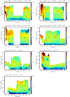 |
Fig. A.1 Same as Fig. 3, but for C2H6. |
| In the text | |
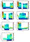 |
Fig. A.2 Same as Fig. 3, but for HCN. |
| In the text | |
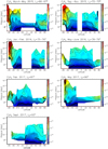 |
Fig. A.3 Same as Fig. 3, but for C4H2. |
| In the text | |
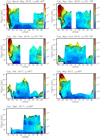 |
Fig. A.4 Same as Fig. 3, but for CH3C2H. |
| In the text | |
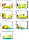 |
Fig. A.5 Same as Fig. 3, but for C3H8. |
| In the text | |
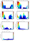 |
Fig. A.6 Same as Fig. 3, but for HC3N. |
| In the text | |
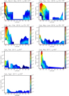 |
Fig. A.7 Same as Fig. 3, but for C6H6. |
| In the text | |
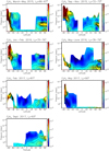 |
Fig. A.8 Same as Fig. 3, but for C2H4. |
| In the text | |
|
Fig. A.9 Haze extinction coefficient (given in cm−1 and representative of 1090 cm−1) meridional cross sections from March 2015 to September 2017. Extinction coefficient is derived from the fit of the 595–660 cm−1 spectral range and scaled to 1090 cm−1 using the spectral dependence derived by Vinatier et al. (2012). Regions without information are represented in white; they correspond to missing data or pressure levels not probed by nadir observations. |
| In the text | |
|
Fig. C.1 Thermal field (top), C2H2 (middle), and HCN (bottom) volume mixing ratio meridional cross sections from March 2015 to September 2017 (from left to right). |
| In the text | |
|
Fig. C.2 C4H2 (top), CH3C2H (middle), and C2H6 (bottom) volume mixing ratio meridional cross sections seasonal changes from March 2015 to September 2017 (from left to right). |
| In the text | |
|
Fig. C.3 HC3N (top), C6H6 (middle), and C3H8 (bottom) volume mixing ratio meridional cross sections seasonal changes from March 2015 to September 2017 (from left to right). |
| In the text | |
|
Fig. C.4 Meridional cross sections of C2H4 volume mixing ratio (top) and haze mass mixing ratio determined from the continuum in the spectral region around 610 cm−1 (FP3, middle) and 1090 cm−1 (FP4, bottom) from March 2015 to September 2017 (from left to right). |
| In the text | |
|
Fig. D.1 Comparison of the aerosol extinction coefficient at 1090 cm−1 derived from CIRS observations in 2015 and 2016 (left column) with those inferred from Cassini ISS Narrow Angle camera at 338 nm (right column) (Seignovert et al. 2020). Extinction is given in cm−1 and a factor 1.22 × 10⁻³ was applied to the extinction coefficient of Seignovert et al. (2020) in order to take into account the aerosol extinction spectral dependence between 338 nm and 1090 cm−1 (Vinatier et al. 2012). |
| In the text | |
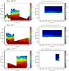 |
Fig. D.2 Same as Fig. D.1, but for 2017. |
| In the text | |
Current usage metrics show cumulative count of Article Views (full-text article views including HTML views, PDF and ePub downloads, according to the available data) and Abstracts Views on Vision4Press platform.
Data correspond to usage on the plateform after 2015. The current usage metrics is available 48-96 hours after online publication and is updated daily on week days.
Initial download of the metrics may take a while.