| Issue |
A&A
Volume 641, September 2020
|
|
|---|---|---|
| Article Number | A104 | |
| Number of page(s) | 10 | |
| Section | Interstellar and circumstellar matter | |
| DOI | https://doi.org/10.1051/0004-6361/202038243 | |
| Published online | 16 September 2020 | |
Studying star-forming processes at core and clump scales: the case of the young stellar object G29.862−0.0044
1
CONICET – Universidad de Buenos Aires. Instituto de Astronomía y Física del Espacio CC 67,
Suc. 28,
1428
Buenos Aires, Argentina
e-mail: This email address is being protected from spambots. You need JavaScript enabled to view it.
2
Isaac Newton Group of Telescopes,
38700
La Palma,
Spain
3
Instituto de Astrofísica de Canarias, Calle Vía Láctea, s/n, 38205 San Cristóbal de La Laguna,
Santa Cruz de Tenerife
38205,
Spain
4
Departamento de Astrofísica, Universidad de La Laguna (ULL),
38205
La Laguna,
Tenerife, Spain
5
Departamento de Astronomía, Universidad de Chile,
Casilla 36-D,
Santiago, Chile
Received:
23
April
2020
Accepted:
13
July
2020
Abstract
Aims. To advance our knowledge of star formation, in addition to statistical studies and large surveys of young stellar objects (YSOs), it is important to carry out detailed studies towards particular objects. Given that massive molecular clumps fragment into cores where star formation takes place, these kinds of studies should be done on different spatial scales. The aim of this work is to investigate the star-forming processes at core and clump scales.
Methods. Using near-infrared (NIR) data obtained with NIRI at the Gemini-North telescope, data of the complex molecular species CH3OCHO and CH3CN obtained from the Atacama Large Millimeter Array (ALMA) database, observations of HCN, HNC, HCO+, and C2H carried out with the Atacama Submillimeter Telescope Experiment (ASTE), and CO data from public surveys observed with the James Clerck Maxwell Telescope (JCMT), we perform a deep study of the YSO G29.862−0.0044 (YSO-G29) at core and clump spatial scales.
Results. The NIR emission shows that YSO-G29 is composed of two nebulosities separated by a dark lane, suggesting a scenario consistent with a typical disc plus jets system, albeit in this case highly asymmetric. The northern nebulosity is open, diffuse, and is divided into two branches, while the southern one is smaller and sharper. They are likely produced by the scattered light in cavities carved out by jets or winds on an infalling envelope of material, which also presents line emission of H2 S(1) 1–0 and 2–1, and [FeII]. The presence of the complex molecular species observed with ALMA confirms that we are mapping a hot molecular core. The CH3CN emission concentrates at the position of the dark lane and appears slightly elongated from southwest to northeast in agreement with the inclination of the system as observed in the NIR. The morphology of the CH3OCHO emission is more complex and extends along some filaments and concentrates in knots and clumps, mainly southwards of the dark lane, suggesting that the southern jet is encountering a dense region. The northern jet is able to flow more freely, generating the more extended features as seen in the NIR. This is in agreement with the redshifted molecular outflow traced by the 12CO J = 3–2 line extending towards the northwest and the lack of a blueshifted outflow. This configuration can be explained by considering that G29-YSO is located at the furthest edge of the molecular clump along the line of sight, which is consistent with the position of the source in the cloud mapped in the C18O J = 3–2 line. The detection of HCN, HNC, HCO+, and C2H allowed us to characterise the dense gas at clump scales, yielding results that are in agreement with the presence of a high-mass protostellar object.
Key words: stars: formation / stars: protostars / ISM: jets and outflows / ISM: molecules
© ESO 2020
1 Introduction
It is known that massive stars form deeply embedded in cores of giant molecular clouds, places with very high visual absorption due to the presence of abundant interstellar dust. They form on relatively short timescales, at distances greater than the nearest examples of their low-mass counterparts (Hill et al. 2005). Additionally, given that massive stars tend to form in clusters, the regions in which they form are very complex. These issues make it difficult to obtain useful observational data towards individual massive young stellar objects (MYSOs), and hence, our knowledge about the physics of the massive star formation is far from being complete.
MYSOs produce massive molecular outflows (Kurtz et al. 2000; Arce et al. 2007) which contribute to the removal of excess angular momentum from accreted matter and to the dispersal of infalling circumstellar envelopes (Reipurth & Bally 2001; Preibisch et al. 2003). The study of molecular outflows and accretion processes adds to our understanding of the formation of stars of all masses, in particular of high-mass stars (Yang et al. 2018). Therefore, even though the molecular outflows are frequently confused with the molecular gas of the clump in which the MYSOs are embedded, and with gas associated with other nearby sources, it is worth making efforts in studying them. Hence, besides the large surveys and statistical studies of YSOs and massive outflows, it is also necessary to do detailed studies towards particular objects. Moreover, given that massive clumps are known to fragment into cores where star formation takes place (Motte et al. 2018), this kind of study should be done at different spatial scales, characterising the physical and chemical properties of the star-forming regions at clump and core scales (see Schwörer et al. 2019 and previous papers of the series).
Nowadays there are very useful surveys of MYSOs and molecular outflows generated from sources of the Red MSX Source (RMS) survey database (Lumsden et al. 2013). For instance, Maud et al. (2015a), based on C18 O data, analysed a large sample of massive star-forming cores and then Maud et al. (2015b) studied associated molecular outflows using 12CO and 13CO data. More recently, Yang et al. (2018) present the largest survey of outflows within the Galactic plane using 13CO and C18O data. These surveys provide large and homogeneous samples of sources that allow us to select particular MYSOs to perform dedicated observations for deeper and more detailed studies on individual objects.
In this work we focus on YSO G29.862−0.044 (hereafter YSO-G29), which is embedded in the southern portion of a molecular cloud located at a distance of about 6.2 kpc, related to the star-forming region G29.96−0.02 (W43-South, Carlhoff et al. 2013). This YSO is likely embedded in a dense cold dust clump traced by both 870 μm and 1.1 mmemissions (Urquhart et al. 2014 and Rosolowsky et al. 2010, respectively). YSO-G29 presents NH3 and methanol maser emission at vLSR ~ 101 km s−1 (Urquhart et al. 2011; Pestalozzi et al. 2005), and according to Li et al. (2016), who analyse 12CO and 13CO J = 1–0 data, only a red molecular outflow is observed, which has an estimated mass of 14 M⊙. Yang et al. (2018), based on an analysis of the 13CO and C18O J = 3–2 emission, report velocity ranges for the blue and red wings in the 13CO spectra of 94.7–100.2 and 103.2–106.2 km s−1, respectively, suggesting the presence of blue and red outflows. However, these latter authors do not determine any outflow parameter for this source, probably due to the confusion with the ambient molecular gas and/or with the cold dust clump in which the YSO is likely embedded.
We present new high-resolution near-infrared (NIR) data obtained with NIRI at the Gemini-North telescope and an analysis of Atacama Large Millimeter Array (ALMA) data towards YSO-G29 to study in detail the source and its surroundings at core scales. Additionally, observations of HCN, HNC, HCO+, and C2H obtained with the Atacama Submillimeter Telescope Experiment (ASTE), and an analysis of CO public data are presented to study the molecular environment of YSO-G29 at clump scales.
2 Data and data reduction
2.1 Near-infrared data
The images were acquired with the Near InfraRed Imager and Spectrometer (NIRI; Hodapp et al. 2003) at the Gemini-North 8.2-m telescope. The observations were carried out on July 2017 in queue mode (Band-1 Program GN-2017B-Q-25). NIRI was used with the f/6 camera that provides a plate scale of 0.′′ 117 pix−1 in a field of view of 120′′ ×120′′.
The extended source in the NIR occupies a large fraction of the field and the background exhibits nebular emission. Therefore, in addition to the dithering pattern on-source, it was also necessary to perform off-source observations in each filter for sky subtraction.
The NIRI data were reduced with DRAGONS, the Gemini’s new Python-base data reduction platform (version 2.1.0), and Theli (Schirmer 2013; Erben et al. 2005). The absolute astrometric solution was made using targets in the field of the 2MASS 6X Point Source Working Database Catalog (Cutri et al. 2012).
Table 1 lists the filters used with their central wavelength and width, the effective spatial resolution measured as the average full width at half maximum (FWHM) of point sources in the final stacked images, and the effective exposure times of the final images. We note that all images presented in this paper were normalised to 1 s. No flux calibration was made.
The H-cont image was used to subtract the continuum of [FeII] and the K-cont image was used to subtract the continuum of H2 1–0 S(1), H2 2–1 S(1), and CO 2–0 (bh). For the continuum subtraction the images were convolved with a Gaussian kernel to achieve a similar PSF for the point sources at the central area of both images. In this process the effective resolution of both images was degraded to a similar value. After convolution the images were scaled to account for the differences in filter width and throughput, and other effectsderived from possibly variable observing conditions. The scale factors were derived from aperture photometry of point sources in the central part of the field.
Near-infrared bands observed with NIRI at Gemini-North.
2.2 Molecular data
The molecular analysis was done at two different spatial scales: we used ALMA data of the complex molecular species CH3OCHO and CH3CN at high angular resolution. To study the molecular environment of YSO-G29 at moderate angular resolutions we used 12CO and C18O J = 3–2 data obtained from a public database, and dedicated observations of HCN, HNC, HCO+ J = 4–3, and C2H N = 4–3 from ASTE.
2.2.1 ALMA data
Data cubes of the emission of methyl formate (CH3OCHO) and methyl cianide (CH3CN) with centralfrequencies at 226.71 and 239.01 GHz, respectively, were obtained from the ALMA Science Archive1 (Project code: 2015.1.01312.S). The beam size of both data cubes is 0.′′78 × 0.′′ 60, which provides a spatial resolution of about 0.02 pc (~4000 au) at the distance of 6.2 kpc. The velocity spectral resolution is 1.5 km s−1. The Common Astronomy Software Applications (CASA) was used to handle these data. The task imcontsub was used to subtract the continuum from the spectral lines.
2.2.2 12CO and C18O data
The 12CO and C18O J = 3–2 data were obtained from the CO High-Resolution Survey (COHRS) and 13CO/C18O (J = 3–2) Heterodyne Inner Milky Way Plane Survey (CHIMPS), two public databases of observations carried out with the 15m James Clerck Maxwell Telescope (JCMT) in Hawaii. The angular and spectral resolutions are 14′′ and 1 km s−1 in the case of 12CO (Dempsey et al. 2013), and 15′′ and 0.5 km s−1 for the C18O (Rigby et al. 2016) providing a spatial resolution of about 0.4 pc at the distance of 6.2 kpc. The intensities of both data sets are on the  scale, and the main beam efficiency ηmb = 0.61 for the 12CO, and ηmb = 0.72 for the C18O was used to convert
  to main beam brightness temperature,
  (Buckle et al. 2009).
2.2.3 ASTE observations
The observations of HCN, HNC, HCO+ J = 4–3, and C2H N = 4–3 were carried out on August 2019 with the 10m ASTE telescope at the central frequencies 354.505, 362.630, 356.734, and 349.337 GHz, respectively. The DASH 345 GHz band receiver was used with the FX-type spectrometer WHSF (bandwidth of 2018 MHz and spectral resolution of 1 MHz). The velocity resolution is 0.86 km s−1, and the beam size (FWHM) is 22′′, which provides a spatial resolution of about 0.6 pc at the distance of 6.2 kpc. The typical system temperature was about 300 K and the main beam efficiency ηmb ~ 0.65. The observed pointing of the four molecular species was: +18h45m59.5s, − 02°45′04.1′′ (J2000), with a pointing accuracy of about 3′′. The integration times were: 30, 36, 20, and 19 min for the HCN, HNC, HCO+, and C2H, respectively.
The data were reduced with NEWSTAR2. The line base fitting was done using just a first-order polynomial and the resulting rms noise level was about 200 mK for all lines.
3 Results
Taking into account that the spatial scales corresponding to cores and clumps in which massive stars are born are < 0.2 and ~ 0.5 pc, respectively (Motte et al. 2018), we present the results separately, according to their spatial scale: in Sect. 3.1 we present the results obtained from the Gemini NIR observations and ALMA data at core scales, and in Sect. 3.2, we show the results obtained from the ASTE observations and the CO surveys at clumps scale.
3.1 At core scales
Figure 1 shows a three-colour image of the emission in the JHK broad bands of a region of about 55′′ ×45′′ towards YSO-G29. Regarding the narrow bands, Fig. 2 shows the emission of the H-cont and K-cont bands, while Fig. 3 displays the emission of the [FeII], H2 1–0 S(1) and 2–1 S(1), and CO 2–0 (bh) lines with continuum (left panel), and continuum subtracted (right panel), except for the CO 2–0 (bh) as the resulting continuum subtracted image quality is poor and hence not reliable. In the continuum-subtracted images some residuals of point sources remained due to differences in the point spread functions (PSFs) of the targets in the final stacked images. Such PSF differences may arise as the combined effect of field distortions in NIRI and the relatively large offsets (~ 42 arcsec) between images resulting from the dithering pattern applied when observing. These features mainly affect point sources but their effect at the scales of extended sources is diluted.
Figure 4 displays three maps obtained from the ALMA data: the continuum map at 1.3 mm and integrated emission maps of the complex molecules CH3OCHO 20(2,19)–19(2,18)E and CH3CN J = 13–12 K = 0. For comparison, contours of the NIR Ks-emission obtained with Gemini are superimposed to each map. Table 2 presents the parameters obtained from the main core observed at 1.3 mm, that is, the more intense core located almost at the centre of the NIR emission.
To analyse the morphology of the molecular core along the line of sight and its kinematical features, Fig. 5 presents a channel map of the CH3OCHO 20(2,19)–19(2,18)E from 95 to 107 km s−1 each 1.5 km s−1, and the same is presented in Fig. 6 for the CH3CN J = 13–12 K = 0 line from 96.5 to 108.5 km s−1, in which the last two panels correspond to emission from the J = 13–12 K = 1 line. It is important to remark that the other CH3CN K projections exhibit exactly the same morphology as K = 0 in the integrated channel maps.
Figure 7 shows in a three-colour image the NIRI Ks emission in red and the integrated emission of the CH3OCHO and CH3CN in green and blue, respectively. Two contours of the integrated CH3CN at 1.5 and 5.0 Jy beam−1 km s−1 levels are also included.
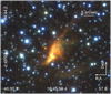 |
Fig. 1 Three-colour image of a 55′′×45′′ region towards YSO-G29 with the JHK broad-band emission presented in blue, green, and red, respectively. |
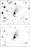 |
Fig. 2 Top: emission of the H-cont narrow band (at 1.570 μm). Bottom: emission of the K-cont narrow band (at 2.097 μm). |
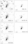 |
Fig. 3 From top to bottom: emission of the [FeII] (at 1.644 μm), H2 1–0 S(1) (at 2.2139 μm), H2 2–1 S(1) (at 2.2465 μm), and CO 2–0 (bh) (at 2.289 μm) with continuum (left column) and continuum subtracted (right column) except for the CO 2–0 (bh). |
Parameters of the central core observed from the ALMA continuum emission at 1.3 mm.
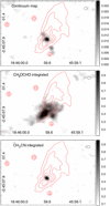 |
Fig. 4 Top: ALMA continuum map at 1.3 mm of G29-YSO. The colour scale is in Jy beam−1, and the rms noise level is 0.001 Jy beam−1. Middle and bottom panels: maps of the CH3OCHO 20(2,19)–19(2,18)E emission integrated between 95 and 107 km s−1, and the CH3CN J = 13–12 K = 0 emission integrated between 98 and 105 km s−1, respectively. The colour scale is in Jy beam−1 km s−1. The rms noise levels are 0.10, and 0.05 Jy beam−1 km s−1, respectively.The beam of the ALMA data is included in the top right corner of each panel. Red contours correspond to the Ks-emission obtained with Gemini and are included for reference. |
3.1.1 Physical parameters from the CH3CN emission
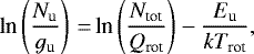
Figure 8 shows an averaged spectrum of the CH3CN J = 13–12 towards G29-YSO. The K projections of the transition are marked. The relevant parameters from the Gaussian fittings presented in Table 3 are the central frequency, the peak intensity (Ipeak), and the integrated flux density (W). The energy of the upper level (Eu) and the line strength of the transition multiplied by the dipolar moment (Sul μ2) are also included. The integrated flux densities were used to construct the rotational diagram (RD) presented in Fig. 9. By assuming LTE conditions, optically thin lines, and a beam filling factor equal to unity, we can estimate the rotational excitation temperature (Trot) and the column density of the CH3CN from the RD analysis (Turner 1991). This analysis is based on a derivation of the Boltzmann equation,
 (1)
(1)
where Nu represents the molecular column density of the upper level of the transition, gu the total degeneracy of the upper level, Ntot the total column density of the molecule, Qrot the rotational partition function, and k the Boltzmann constant.
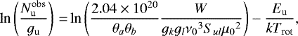
Following Miao et al. (1995), for interferometric observations, the left-hand side of Eq. (1) can also be estimated by,
 (2)
(2)
where  (in cm−2) is the observed column density of the molecule under the conditions mentioned before, θa and θb (in arcsec) are the major and minor axes of the clean beam, respectively, W (in Jy beam−1 km s−1) is the integrated intensity of each K, gk is the K-ladder degeneracy, gl is the degeneracy due to the nuclear spin,ν0 (in GHz) is the rest frequency of the transition, Sul is the line strengthof the transition, and μ0 (in Debye) is the permanent dipole moment of the molecule. The free parameters, (Ntot∕Qrot) and Trot were determined by a linear fitting of Eq. (1) (see Fig. 9). We derive a Trot of about 82 K and, using a tabulated value for Qrot at this temperature, we obtain a CH3CN column density of about 1015 cm−2.
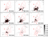 |
Fig. 5 Channel maps of the CH3OCHO 20(2,19)–19(2,18)E. Red contours correspond to the Ks-emission obtained with Gemini and are included for reference. The colour scale is in Jy beam−1 and is shown in the last panel. The beam of the ALMA data is included in the top left corner in each panel. |
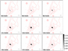 |
Fig. 6 Channel maps of the CH3CN J = 13–12 K = 0. Red contours correspond to the Ks-emission obtained with Gemini and are included for reference. The colour scale is in Jy beam−1 and is shown in the last panel. The beam of the ALMA data is included in the bottom right corner in each panel. The emission at panels 107.0 and 108.5 km s−1 is very likely contaminated with the emission of the line with projection K = 1. |
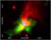 |
Fig. 7 Three-colour image composed of Gemini NIRI Ks emission (red) and the integrated emission of CH3OCHO (green) and CH3CN (blue) as presented in Fig. 4. The black contours are the integrated CH3CN emission at levels 1.5 and 5.0 Jy beam−1 km s−1. The beam of the ALMA data is displayed in the top right corner. |
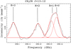 |
Fig. 8 CH3CN J = 13–12 averaged spectrum towards G29-YSO at rest frequency. The K projections of the J line are marked. The single or multiple-component Gaussian fits are shown in red. |
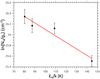 |
Fig. 9 Rotation diagram of the CH3CN J = 13–12 obtained from K = 0, 1, 2, and 3 projections. The red line is the linear fitting. |
3.1.2 Mass and density of the core
We estimatethe mass of gas of the central core from the dust continuum emission at 1.3 mm following Kauffmann et al. (2008),
![Mathematical equation: \begin{eqnarray*} M_{\textrm{gas}}&=&0.12~{M_{\odot}} \left[\textrm{exp}\left(\frac{1.439} {(\lambda/\textrm{mm})(T_{\textrm{dust}}/10~\textrm{K})}\right)-1\right] \\ \nonumber &&\times\left(\frac{\kappa_{\nu}}{0.01~\textrm{cm}^2~\textrm{g}^{-1}}\right)^{-1}\left(\frac{S_{\nu}}\textrm{Jy}\right)\left(\frac{d}{100~\textrm{pc}}\right)^2\left(\frac{\lambda}\textrm{mm}\right)^3,\end{eqnarray*}](/articles/aa/full_html/2020/09/aa38243-20/aa38243-20-eq7.png) (3)
(3)
where Tdust is the dust temperature and κν is the dust opacity per gram of matter at 1.3 mm for which we adopt the value of 0.01 cm2 g−1 (Kauffmann et al. 2008; Ossenkopf & Henning 1994). Assuming LTE conditions (Tkin = Trot), and that the gas and dust are thermally coupled (Tdust = Tkin), and considering the integrated flux intensity Sν = 0.051 Jy at 1.3 mm (see Table 2), we obtain Mgas ~ 8 M⊙. Hence, assuming spherical geometry we can derive a volume density of n(H2) ~ 1 × 106 cm−3.
Additionally, neglecting contributions from magnetic field and surface pressure, we estimate the virial mass using the CH3CN emission and the following equation:
 (4)
(4)
where k = 190 by assuming a density distribution ∝ r−1 (MacLaren et al. 1988), Δv is the line velocity width (FWHM) of the CH3CN emission obtained from the Gaussian fittings presented in Fig. 8, estimated to be about 6.7 km s−1 (the Δv of all K projections of the J = 13–12 transition goes from 5.5 to 8.0 km s−1), and R is the radius, which is equal to approximately 0.01 pc (from the source size presented in Table 2). Thus, we obtain Mvir ~ 70 M⊙.
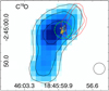 |
Fig. 10 C18O J = 3–2 emission integrated between 99 and 104.5 km s−1. The contour levels are 5, 7, and 10 K km s−1. The red contour corresponds to the 12CO J = 3–2 emission integrated between 104 and 112 km s−1. The red contour levels are 40 and 50 K km s−1. The beam isincluded at the bottom right corner. The yellow contours correspond to the NIR Ks-emission obtained with Gemini. The dashed circle represents the pointing and the beam of the ASTE observations. |
3.2 At clump scales
To study the cloud and the clump in which G29-YSO is embedded, in Fig. 10 we present the integrated C18O J = 3–2 emission between 98.0 and 104.5 km s−1 (the velocity range in which the emission of the C18O extends). Following previous works (see Sect. 1) the 12CO J = 3–2 emission integrated between 104 and 112 km s−1 (the red wing as observed in this line) is displayed in red contours showing the already reported red molecular outflow. In addition, in Fig. 11we present the C18O J = 3–2 spectrum obtained towards the G29-YSO position. By integrating the 12CO in the velocity range corresponding to the blue wing suggested by Yang et al. (2018), it is possible to distinguish a molecular feature associated with the southern portion of the elongated cloud observed in the C18O line, which is coincident with another cold dust clump as observed in ATLASGAL and radio continuum sources (NVSS J184603-024541 and NVSS J184601-024601), showing that it should be molecular gas related to another active region within the same complex. Thus, this blue component in the 12CO cannot be considered as a molecular outflow.
Figure 12 shows the spectra from the emission of the HCO+, HCN, and HNC. Figure 13 shows the spectrum of C2H as observed with ASTE towards the YSO position (dashed green circle in Fig. 10). Table 4 lists the parameters obtained from the Gaussian fitting to each spectrum presented in Figs.11–13. The C2H presents two peaks due to its fine structure components. The central frequency to observe this molecular species was set at 349.337 GHz, which corresponds to the N = 4–3 J = 9/2–7/2 F = 5–4 transition. While each C2H peak was fitted by one Gaussian, it is important to remark that one peak should correspond to the blended C2H (N = 4–3) J = 9/2–7/2 F = 5–4 and 4–3 lines (from which the systemic velocity of 100.98 km s−1 is obtained), and the other to the blended (N = 4–3) J = 7/2–5/2 F = 4–3 and 3–2 lines (see e.g. the NIST data base3). The same occurs with the HCN J = 4–3 line, which is also affected by the hyperfine splitting. The HCN/HNC integrated ratio is ~ 2.3.
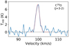 |
Fig. 11 C18O J = 3–2 spectrum from the JCMT data at the G29-YSO position. The red dotted lines are the Gaussian fittings. |
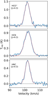 |
Fig. 12 HCO+, HCN, and HNC J = 4–3 observed with ASTE towards G29-YSO. The red dotted lines are the Gaussian fittings. |
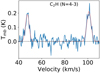 |
Fig. 13 C2H spectrum observed with ASTE towards G29-YSO. The red dotted lines are the Gaussian fittings. |
4 Discussion
As done in Sect. 3, we present separate discussions of the results at the two spatial scales (core and clump) analysed.
4.1 Core scales
The NIR bands show that YSO-G29 is composed of two nebulosities separated by a dark lane (see Figs. 1–3). The dark lane could be due to the presence of an accretion disc or a rotating toroid which may hide the protostar(s), as is usually found towards YSOs observed mainly edge-on (Beltrán & de Wit 2016; Furuya et al. 2008). The NIR emission is highly asymmetric as the northern nebulosity is extended and open, while the southern counterpart is smaller. Overall, the nebulosities seem to be composed of some jet-like structures, suggesting a scenario consistent with the typical disc-jets systems observed over decades generally towards nearby YSOs (e.g. Padgett et al. 1999) and in agreement with the description given for this source in the RMS survey of Lumsden et al. (2013) based on UKIDSS NIR data. However, the high resolution of the NIRI data allows us to distinguish some intriguing features. The jet-like structure extending towards the northwest is divided into two branches. One branch curves towards the west and slightly to the south, generating an M-shaped structure (see mainly the Ks emission displayed in red in Figs. 1 and 7). The other branch extends mainly straight to the north. Diffuse emission is observed between both branches. On the other hand, the southern jet-like feature leans more sharply to the southeast.
It is well known that the NIR emission towards this kind of object arises mainly from scattered light in the material surrounding the protostar(s), emission from warm dust plus atomic and molecular emission lines (e.g. Muzerolle et al. 2013; Bik et al. 2006, 2005; Reipurth et al. 2000). The geometry of the NIR emission presented here is quite similar to that detected towards the protostar L54361 (Muzerolle et al. 2013) and, as the authors proposed, it is probably produced by the scattered light in cavities carved out by one or more jets on an infalling envelope of material.
Most of the structures that are observed in the Ks-band are also present in the H2 1–0 and 2–1 S(1) as shown in the right panel of Fig. 3. The NIR emission from H2 can be generated by either thermal emission in shock fronts or fluorescence excitation by non-ionising UV photons (Martín-Hernández et al. 2008). As those authors mention, in high-density regions (as in this case) a combination of 1–0 (S1)/2–1 (S1) and 1–0 S(1)/3–2 S(3) ratios is necessary to assess the H2 excitation mechanism. Our NIR data set is not complete for specifying this and even though there is no evidence in the NIRI images of a well-collimated H2 structure, as is usually found towards jets (e.g. Dewangan et al. 2015), considering that jets could be curved in certain conditions we cannot discard a contribution from shocks for the observed H2 emission. Additionally, given that the H2 radiative excitation, and hence its emission, should be due to UV photons impinging the molecular gas in cavities carved out by the YSO jets and/or winds (Frank et al. 2014), it makes sense to conclude that the observed features in the H2 are indeed due to the activity of a protostar(s) likely hidden in the dark lane. In general, the [FeII] emission present a similar morphology to that seen for the other bands, but the jet-like structures are much less conspicuous and more diffuse. The origin of this emission could be knots and shock fronts along the regions where the jets propagate (Bally 2007; Davis et al. 2011).
From the analysis of the ALMA data (see Figs. 4–7) we find a well-defined core mapped in the continuum emission at 1.3 mm lying almost at the position of the dark lane of the NIR emission (slightly displaced to the north) and other weaker cores towards the northeast and southwest. The main core has a size of about 4300 au, which is in agreement, together with the measured flux and peak intensity (see Table 2), with the values obtained towards the hot core G31-NE (Beltrán et al. 2018). The CH3CN emission is in perfect spatial coincidence with the central core as observed in 1.3 mm continuum. The CH3OCHO emission is more extended and presents some knots and filament-like features. Both molecular species are usually detected towards hot molecular cores (Bonfand et al. 2017; Fuente et al. 2014; Codella et al. 2013; Olmi et al. 1996). The rotational temperature and column density determined from the rotational diagram of the CH3CN (Trot ~ 82 K and N ~ 1015 cm−2) are in agreement with those determined towards several hot molecular cores (e.g. Araya et al. 2005). The mass of gas and the density obtained for the core agrees with the lowest values obtained in several molecular hot cores that were investigated using the 1.3 mm continuum and CH3CN emission observed with the Submillimeter Array (Hernández-Hernández et al. 2014). A mass about 10 M⊙ is the usually adopted lower limit for the gas mass of a hot molecular core (Cesaroni 2005). Comparing the mass of the core with the bolometric luminosity obtained towards this source, about 4.5 × 10⁴ L⊙ (based on the luminosity of Mottram et al. 2011 corrected to the assumed distance of 6.2 kpc), and following Cesaroni (2005), we can conclude that we are observing a “light” hot molecular core, which implies that the mass of the embedded star is comparable to or greater than the gas mass. Hernández-Hernández et al. (2014) found that most of the Mvir values are greater than Mgas in their hot molecular cores sample, as in our case, and these latter authors propose that this imbalance could be due to the fact that the cores are not in dynamical equilibrium owing to complicated kinematics, and large rotating structures such as toroids and discs among other dynamical processes that will increase the line width and thus the virial mass. We conclude that we are indeed observing a “light” hot molecular core, which probably contains a rotating toroid/disc.
It is worth noting that the CH3CN emission appears slightly elongated from southwest to northeast (see contours in Fig. 7 and the channel map at 101.0 km s−1 in Fig. 6) in agreement with the inclination of the system as observed at NIR wavelengths. Taking into account that this feature coincides with the dark lane observed in NIR, it is also possible that part of the emission of CH3CN traces a toroid, as was suggested for the hot molecular core G31.41+0.31 based on observations of CH3CN J = 12–11 (Cesaroni et al. 2011). Indeed, this molecular species is also detected towards protoplanetary discs (Loomis et al. 2018).
The morphology of the CH3OCHO emission is more complex than the morphology of the CH3CN emission. As observed in the channel maps (Fig. 5), the CH3OCHO emission extends along some filaments and concentrates in knots and clumps similar to that found in the star-forming complex Sagittarius B2(N) (Schwörer et al. 2019). In that case, the authors discarded the possibility that the CH3OCHO filaments were due to outflows or explosive events like the one seen in Orion KL by Bally et al. (2017), because such filaments are curved and bent. In G29-YSO, we observe that at the first channel map (at 95 km s−1 in Fig. 5) a straightforward and collimated structure extends towards the southeast in coincidence with the southern NIR nebulosity. At the two last channel maps (at 105.5 and 107.0 km s−1) two weaker filaments are observed: one elongated and pointing to the northern NIR nebulosity, and the other one pointing to the M-shaped structure as seen in the NIR emission. These structures mapped in the CH3OCHO emission suggest expanding motions of molecular gas from the region of the dark lane where protostar(s) should be embedded, indicating outflow activity in the region, in agreement with the scenario pictured from the NIR data. The others CH3OCHO structures present core morphology. In particular, towards the southeast, a core of this molecular species coincides with a core observed in the continuum emission at 1.3 mm.
The CH3OCHO emission shows the presence of molecular material mainly southwards, in coincidence with the region where the NIR emission presents a sharper structure than in the northern case. This suggests that the jets and/or stellar winds are encountering a dense region, while towards the north they can flow more freely, generating the more extended features seen in NIR. Additionally, it is worth noting that the distribution of the CH3OCHO towards the northwest could explain the lack of NIR emission in the region below the M-shaped structure described above (see Fig. 7).
4.2 Clump scales
Figure 10 shows that YSO-G29 is located at the northwestern portion of a molecular clump belonging to an elongated cloud as mapped in the C18O J = 3–2 line. The redshifted molecular outflow traced by the 12CO J = 3–2 line (also detected in the 12CO J = 1–0 line by Li et al. 2016) extends towards the northwest, the same direction as the northwestern nebulosity detected in the NIR observations. As mentioned above, and in agreement with previous works, we did not detect any blueshifted molecular outflow. One possible explanation is that the YSO is located in the furthest edge of the molecular clump along the line of sight, and thus, the redshifted molecular outflow freely flows to the exterior of the clump (and we can observe it), while the blueshifted counterpart goes into the clump, making its detection difficult. This is consistent with the less intense and less extended southern NIR emission in comparison with the northern one and with the spatial distribution of the CH3OCHO emission discussed above.
The molecular species observed with ASTE confirm the presence of high-density gas towards YSO-G29. The detection of HCO+ is consistent with the presence of molecular outflows (e.g. Sánchez-Monge et al. 2013; Rawlings et al. 2004), and the HCN and HNC, indeed tracers of high-density gas, can be used to trace the evolutionary stages of star-forming regions (Graninger et al. 2014). A statistical tendency of increasing HCN/HNC abundance ratio was found from starless clumps (values about unity) to UC HII regions (values about 9) by Jin et al. (2015). If we consider that the HCN/HNC integrated line ratio resembles the abundance ratio (integration line ratio variations are driven by similar changes in the abundance ratio; Hacar et al. 2020), according to Jin et al. (2015), our value of 2.3 would correspond to an active IR dark cloud core (aIRDCc). Following Hacar et al. (2020), who show that the HCN/HNC integrated line ratio can be used to estimate the kinetic temperature (TK) of the gas, using their Eq. (3), we obtain TK ~ 23 K towards G29-YSO. This value is in quite good agreement with the dust temperature at the YSO position (Tdust ~ 26 K) obtained from the dust temperature map4 which was derived by applying the PPMAP procedure to the Hi-GAL maps in the wavelength range 70–500 μm (Marsh et al. 2017). Our TK obtained from the HCN/HNC ratio also agrees with TK ~ 21.7 K estimated from the NH3 emission (Wienen et al. 2012) towards the ATLASGAL cold high-mass clump G29.85-0.06 which lies at the southern portion of the molecular cloud displayed in Fig. 10, suggesting that the whole molecular cloud, analysed at clump scales, has a temperature of about 25 K. As in Hacar et al. (2020), who used the HCN and HNC J = 1–0 line, we also find a very good correlation between the TK derived from the HCN/HNC ratio (in our case using the J = 4–3 line) and the Tdust obtained from IR data.
The C2H is observed towards several types of interstellar regions (e.g. Nagy et al. 2015 and references therein), and particularly, it seems to be almost omnipresent along the different evolutionary stages of massive star formation (Beuther et al. 2008). As photodissociation of larger carbon-chain molecules and polycyclic aromatic hydrocarbons (PAHs) is one of its possible formation processes, C2H is known to be a good tracer of dense photodissociation regions (PDRs). Beuther et al. (2008) observed an increase in the C2H line widths with the evolutionary stage of the star-forming regions, with values of 2.8 for infrared dark clouds (IRDCs), 3.1 km s−1 for high-mass protostellar objects (HMPOs), and 5.5 km s−1 for UC HII regions. The values obtained towards YSO-G29 are consistent with HMPOs, which is in quite good agreement with the results obtained from the HCN and HNC observations described above. As pointed out by Jin et al. (2015), this is because the averaged HCN and HNC spectra of a IRDCs and HMPOs appear to have similar peak intensities and line widths.
5 Concluding remarks
A complete understanding of the processes involved in the formation of the stars requires detailed multi-wavelength studies of individual objects at different spatial scales. In this work, using NIR and molecular line data we perform a deep study of the young stellar object G29.862−0.0044 relating the core and clump scales. The NIR emission shows a likely disc–jet system. The study of the molecular gas at both spatial scales suggests the presence of a hot molecular core. The gas temperature at core and clump scale is about 80 and 25 K, respectively, showing the presence of an internal heating source.
YSO-G29 exhibits a conspicuous asymmetric morphology at both spatial scales. The molecular outflow at clump scale is monopolar with the red lobe located towards the north. The NIR and the CH3OCHO molecular emissions, which map the core scale, suggest a scenario where the jet has flowed more freely towards the north in agreement with the direction of the red lobe of the molecular outflow. Interestingly, unlike other studies at NIR bands towards other sources in which the redshifted jet was not detected due to extinction effects, in this work, this jet appears as the brightest feature, showing that this asymmetry cannot be due to the extinction. We observe that at core scale, the jet or outflow activity is markedly asymmetric but not monopolar. This could be due to a highly inhomogeneous medium, which has consequences at the larger spatial scales.
Acknowledgments
We thank the anonymous referee for her/his fruitful comments. M.B.A. is a doctoral fellow of CONICET, Argentina. S.P. and M.O. are members of the Carrera del Investigador Científico of CONICET, Argentina. M.R. wishes to acknowledge support from CONICYT (CHILE) through FONDECYT grant No1190684 and partial support from CONICYT project Basal AFB-170002. This paper makes use of the following ALMA data: ADS/JAO.ALMA#2015.1.01312.S. ALMA is a partnership of ESO (representing its member states), NSF (USA) and NINS (Japan), together with NRC (Canada), MOST and ASIAA (Taiwan), and KASI (Republic of Korea), in cooperation with the Republic of Chile. The Joint ALMA Observatory is operated by ESO, AUI/NRAO and NAOJ. The ASTE project is led by Nobeyama Radio Observatory (NRO), a branch of National Astronomical Observatory of Japan (NAOJ), in collaboration with University of Chile, and Japanese institutes including University of Tokyo, Nagoya University, Osaka Prefecture University, Ibaraki University, Hokkaido University, and the Joetsu University of Education.
References
- Araya, E., Hofner, P., Kurtz, S., Bronfman, L., & DeDeo, S. 2005, ApJS, 157, 279 [NASA ADS] [CrossRef] [Google Scholar]
- Arce, H. G., Shepherd, D., Gueth, F., et al. 2007, Protostars and Planets V (Tucson, AZ: University of Arizona Press), 245 [Google Scholar]
- Bally, J. 2007, Ap&SS, 311, 15 [Google Scholar]
- Bally, J., Ginsburg, A., Arce, H., et al. 2017, ApJ, 837, 60 [NASA ADS] [CrossRef] [Google Scholar]
- Beltrán, M. T., & de Wit, W. J. 2016, A&ARv, 24, 6 [NASA ADS] [CrossRef] [Google Scholar]
- Beltrán, M. T., Cesaroni, R., Rivilla, V. M., et al. 2018, A&A, 615, A141 [NASA ADS] [CrossRef] [EDP Sciences] [Google Scholar]
- Beuther, H., Semenov, D., Henning, T., & Linz, H. 2008, ApJ, 675, L33 [NASA ADS] [CrossRef] [Google Scholar]
- Bik, A., Kaper, L., Hanson, M. M., & Smits, M. 2005, A&A, 440, 121 [NASA ADS] [CrossRef] [EDP Sciences] [Google Scholar]
- Bik, A., Kaper, L., & Waters, L. B. F. M. 2006, A&A, 455, 561 [NASA ADS] [CrossRef] [EDP Sciences] [Google Scholar]
- Bonfand, M., Belloche, A., Menten, K. M., Garrod, R. T., & Müller, H. S. P. 2017, A&A, 604, A60 [NASA ADS] [CrossRef] [EDP Sciences] [Google Scholar]
- Buckle, J. V., Hills, R. E., Smith, H., et al. 2009, MNRAS, 399, 1026 [NASA ADS] [CrossRef] [Google Scholar]
- Carlhoff, P., Nguyen Luong, Q., Schilke, P., et al. 2013, A&A, 560, A24 [NASA ADS] [CrossRef] [EDP Sciences] [Google Scholar]
- Cesaroni, R. 2005, IAU Symp., 227, 59 [NASA ADS] [CrossRef] [Google Scholar]
- Cesaroni, R., Beltrán, M. T., Zhang, Q., Beuther, H., & Fallscheer, C. 2011, A&A, 533, A73 [NASA ADS] [CrossRef] [EDP Sciences] [Google Scholar]
- Codella, C., Beltrán, M. T., Cesaroni, R., et al. 2013, A&A, 550, A81 [NASA ADS] [CrossRef] [EDP Sciences] [Google Scholar]
- Cutri, R. M., Skrutskie, M. F., van Dyk, S., et al. 2012, VizieR Online Data Catalog: II/281 [Google Scholar]
- Davis, C. J., Cervantes, B., Nisini, B., et al. 2011, A&A, 528, A3 [NASA ADS] [CrossRef] [EDP Sciences] [Google Scholar]
- Dempsey, J. T., Thomas, H. S., & Currie, M. J. 2013, ApJS, 209, 8 [NASA ADS] [CrossRef] [Google Scholar]
- Dewangan, L. K., Mayya, Y. D., Luna, A., & Ojha, D. K. 2015, ApJ, 803, 100 [CrossRef] [Google Scholar]
- Erben, T., Schirmer, M., Dietrich, J. P., et al. 2005, Astron. Nachr., 326, 432 [NASA ADS] [CrossRef] [Google Scholar]
- Frank, A., Ray, T. P., Cabrit, S., et al. 2014, Protostars and Planets VI, eds. H. Beuther, R. S. Klessen, C. P. Dullemond, & T. Henning (Tucson, AZ: University of Arizona Press), 451 [Google Scholar]
- Fuente, A., Cernicharo, J., Caselli, P., et al. 2014, A&A, 568, A65 [NASA ADS] [CrossRef] [EDP Sciences] [Google Scholar]
- Furuya, R. S., Cesaroni, R., Takahashi, S., et al. 2008, ApJ, 673, 363 [NASA ADS] [CrossRef] [Google Scholar]
- Graninger, D. M., Herbst, E., Öberg, K. I., & Vasyunin, A. I. 2014, ApJ, 787, 74 [NASA ADS] [CrossRef] [Google Scholar]
- Hacar, A., Bosman, A. D., & van Dishoeck, E. F. 2020, A&A, 635, A4 [CrossRef] [EDP Sciences] [Google Scholar]
- Hernández-Hernández, V., Zapata, L., Kurtz, S., & Garay, G. 2014, ApJ, 786, 38 [NASA ADS] [CrossRef] [Google Scholar]
- Hill, T., Burton, M. G., Minier, V., et al. 2005, MNRAS, 363, 405 [NASA ADS] [CrossRef] [Google Scholar]
- Hodapp, K. W., Jensen, J. B., Irwin, E. M., et al. 2003, PASP, 115, 1388 [NASA ADS] [CrossRef] [Google Scholar]
- Jin, M., Lee, J.-E., & Kim, K.-T. 2015, ApJS, 219, 2 [NASA ADS] [CrossRef] [Google Scholar]
- Kauffmann, J., Bertoldi, F., Bourke, T. L., Evans, N. J., I., & Lee, C. W. 2008, A&A, 487, 993 [NASA ADS] [CrossRef] [EDP Sciences] [Google Scholar]
- Kurtz, S., Cesaroni, R., Churchwell, E., Hofner, P., & Walmsley, C. M. 2000, Protostars and Planets IV (Tucson, AZ: University of Arizona Press), 299 [Google Scholar]
- Li, F. C., Xu, Y., Wu, Y. W., et al. 2016, AJ, 152, 92 [CrossRef] [Google Scholar]
- Loomis, R. A., Cleeves, L. I., Öberg, K. I., et al. 2018, ApJ, 859, 131 [NASA ADS] [CrossRef] [Google Scholar]
- Lumsden, S. L., Hoare, M. G., Urquhart, J. S., et al. 2013, ApJS, 208, 11 [NASA ADS] [CrossRef] [Google Scholar]
- MacLaren, I., Richardson, K. M., & Wolfendale, A. W. 1988, ApJ, 333, 821 [NASA ADS] [CrossRef] [Google Scholar]
- Marsh, K. A., Whitworth, A. P., Lomax, O., et al. 2017, MNRAS, 471, 2730 [Google Scholar]
- Martín-Hernández, N. L., Bik, A., Puga, E., Nürnberger, D. E. A., & Bronfman, L. 2008, A&A, 489, 229 [NASA ADS] [CrossRef] [EDP Sciences] [Google Scholar]
- Maud, L. T., Lumsden, S. L., Moore, T. J. T., et al. 2015a, MNRAS, 452, 637 [NASA ADS] [CrossRef] [Google Scholar]
- Maud, L. T., Moore, T. J. T., Lumsden, S. L., et al. 2015b, MNRAS, 453, 645 [NASA ADS] [CrossRef] [Google Scholar]
- Miao, Y., Mehringer, D. M., Kuan, Y.-J., & Snyder, L. E. 1995, ApJ, 445, L59 [NASA ADS] [CrossRef] [Google Scholar]
- Motte, F., Bontemps, S., & Louvet, F. 2018, ARA&A, 56, 41 [NASA ADS] [CrossRef] [Google Scholar]
- Mottram, J. C., Hoare, M. G., Davies, B., et al. 2011, ApJ, 730, L33 [NASA ADS] [CrossRef] [Google Scholar]
- Muzerolle, J., Furlan, E., Flaherty, K., Balog, Z., & Gutermuth, R. 2013, Nature, 493, 378 [NASA ADS] [CrossRef] [Google Scholar]
- Nagy, Z., Ossenkopf, V., Van der Tak, F. F. S., et al. 2015, A&A, 578, A124 [NASA ADS] [CrossRef] [EDP Sciences] [Google Scholar]
- Olmi, L., Cesaroni, R., Neri, R., & Walmsley, C. M. 1996, A&A, 315, 565 [NASA ADS] [Google Scholar]
- Ossenkopf, V.,& Henning, T. 1994, A&A, 291, 943 [Google Scholar]
- Padgett, D. L., Brandner, W., Stapelfeldt, K. R., et al. 1999, AJ, 117, 1490 [NASA ADS] [CrossRef] [Google Scholar]
- Pestalozzi, M. R., Minier, V., & Booth, R. S. 2005, A&A, 432, 737 [NASA ADS] [CrossRef] [EDP Sciences] [Google Scholar]
- Preibisch, T., Balega, Y. Y., Schertl, D., & Weigelt, G. 2003, A&A, 412, 735 [NASA ADS] [CrossRef] [EDP Sciences] [Google Scholar]
- Rawlings, J. M. C., Redman, M. P., Keto, E., & Williams, D. A. 2004, MNRAS, 351, 1054 [NASA ADS] [CrossRef] [Google Scholar]
- Reipurth, B., & Bally, J. 2001, ARA&A, 39, 403 [NASA ADS] [CrossRef] [Google Scholar]
- Reipurth, B., Yu, K. C., Heathcote, S., Bally, J., & Rodríguez, L. F. 2000, AJ, 120, 1449 [NASA ADS] [CrossRef] [Google Scholar]
- Rigby, A. J., Moore, T. J. T., Plume, R., et al. 2016, MNRAS, 456, 2885 [NASA ADS] [CrossRef] [Google Scholar]
- Rosolowsky, E., Dunham, M. K., Ginsburg, A., et al. 2010, ApJS, 188, 123 [NASA ADS] [CrossRef] [Google Scholar]
- Sánchez-Monge, Á., López-Sepulcre, A., Cesaroni, R., et al. 2013, A&A, 557, A94 [NASA ADS] [CrossRef] [EDP Sciences] [Google Scholar]
- Schirmer, M. 2013, ApJS, 209, 21 [NASA ADS] [CrossRef] [Google Scholar]
- Schwörer, A., Sánchez-Monge, Á., Schilke, P., et al. 2019, A&A, 628, A6 [NASA ADS] [CrossRef] [EDP Sciences] [Google Scholar]
- Turner, B. E. 1991, ApJS, 76, 617 [NASA ADS] [CrossRef] [Google Scholar]
- Urquhart, J. S., Morgan, L. K., Figura, C. C., et al. 2011, MNRAS, 418, 1689 [NASA ADS] [CrossRef] [Google Scholar]
- Urquhart, J. S., Moore, T. J. T., Csengeri, T., et al. 2014, MNRAS, 443, 1555 [NASA ADS] [CrossRef] [Google Scholar]
- Wienen, M., Wyrowski, F., Schuller, F., et al. 2012, A&A, 544, A146 [NASA ADS] [CrossRef] [EDP Sciences] [Google Scholar]
- Yang, A. Y., Thompson, M. A., Urquhart, J. S., & Tian, W. W. 2018, ApJS, 235, 3 [NASA ADS] [CrossRef] [Google Scholar]
Reduction software based on AIPS developed at NRAO, extended to treat single dish data with a graphical user interface (GUI).
All Tables
Parameters of the central core observed from the ALMA continuum emission at 1.3 mm.
All Figures
|
Fig. 1 Three-colour image of a 55′′×45′′ region towards YSO-G29 with the JHK broad-band emission presented in blue, green, and red, respectively. |
| In the text | |
|
Fig. 2 Top: emission of the H-cont narrow band (at 1.570 μm). Bottom: emission of the K-cont narrow band (at 2.097 μm). |
| In the text | |
|
Fig. 3 From top to bottom: emission of the [FeII] (at 1.644 μm), H2 1–0 S(1) (at 2.2139 μm), H2 2–1 S(1) (at 2.2465 μm), and CO 2–0 (bh) (at 2.289 μm) with continuum (left column) and continuum subtracted (right column) except for the CO 2–0 (bh). |
| In the text | |
|
Fig. 4 Top: ALMA continuum map at 1.3 mm of G29-YSO. The colour scale is in Jy beam−1, and the rms noise level is 0.001 Jy beam−1. Middle and bottom panels: maps of the CH3OCHO 20(2,19)–19(2,18)E emission integrated between 95 and 107 km s−1, and the CH3CN J = 13–12 K = 0 emission integrated between 98 and 105 km s−1, respectively. The colour scale is in Jy beam−1 km s−1. The rms noise levels are 0.10, and 0.05 Jy beam−1 km s−1, respectively.The beam of the ALMA data is included in the top right corner of each panel. Red contours correspond to the Ks-emission obtained with Gemini and are included for reference. |
| In the text | |
|
Fig. 5 Channel maps of the CH3OCHO 20(2,19)–19(2,18)E. Red contours correspond to the Ks-emission obtained with Gemini and are included for reference. The colour scale is in Jy beam−1 and is shown in the last panel. The beam of the ALMA data is included in the top left corner in each panel. |
| In the text | |
|
Fig. 6 Channel maps of the CH3CN J = 13–12 K = 0. Red contours correspond to the Ks-emission obtained with Gemini and are included for reference. The colour scale is in Jy beam−1 and is shown in the last panel. The beam of the ALMA data is included in the bottom right corner in each panel. The emission at panels 107.0 and 108.5 km s−1 is very likely contaminated with the emission of the line with projection K = 1. |
| In the text | |
|
Fig. 7 Three-colour image composed of Gemini NIRI Ks emission (red) and the integrated emission of CH3OCHO (green) and CH3CN (blue) as presented in Fig. 4. The black contours are the integrated CH3CN emission at levels 1.5 and 5.0 Jy beam−1 km s−1. The beam of the ALMA data is displayed in the top right corner. |
| In the text | |
|
Fig. 8 CH3CN J = 13–12 averaged spectrum towards G29-YSO at rest frequency. The K projections of the J line are marked. The single or multiple-component Gaussian fits are shown in red. |
| In the text | |
|
Fig. 9 Rotation diagram of the CH3CN J = 13–12 obtained from K = 0, 1, 2, and 3 projections. The red line is the linear fitting. |
| In the text | |
|
Fig. 10 C18O J = 3–2 emission integrated between 99 and 104.5 km s−1. The contour levels are 5, 7, and 10 K km s−1. The red contour corresponds to the 12CO J = 3–2 emission integrated between 104 and 112 km s−1. The red contour levels are 40 and 50 K km s−1. The beam isincluded at the bottom right corner. The yellow contours correspond to the NIR Ks-emission obtained with Gemini. The dashed circle represents the pointing and the beam of the ASTE observations. |
| In the text | |
|
Fig. 11 C18O J = 3–2 spectrum from the JCMT data at the G29-YSO position. The red dotted lines are the Gaussian fittings. |
| In the text | |
|
Fig. 12 HCO+, HCN, and HNC J = 4–3 observed with ASTE towards G29-YSO. The red dotted lines are the Gaussian fittings. |
| In the text | |
|
Fig. 13 C2H spectrum observed with ASTE towards G29-YSO. The red dotted lines are the Gaussian fittings. |
| In the text | |
Current usage metrics show cumulative count of Article Views (full-text article views including HTML views, PDF and ePub downloads, according to the available data) and Abstracts Views on Vision4Press platform.
Data correspond to usage on the plateform after 2015. The current usage metrics is available 48-96 hours after online publication and is updated daily on week days.
Initial download of the metrics may take a while.