| Issue |
A&A
Volume 641, September 2020
|
|
|---|---|---|
| Article Number | A57 | |
| Number of page(s) | 22 | |
| Section | Interstellar and circumstellar matter | |
| DOI | https://doi.org/10.1051/0004-6361/202037900 | |
| Published online | 09 September 2020 | |
The abundance of S- and Si-bearing molecules in O-rich circumstellar envelopes of AGB stars★,★★
1
Instituto de Física Fundamental, CSIC,
C/ Serrano 123,
28006,
Madrid, Spain
e-mail: sarah.massalkhi@csic.es
2
Department of Space, Earth and Environment, Chalmers University of Technology, Onsala Space Observatory,
439 92
Onsala, Sweden
Received:
6
March
2020
Accepted:
22
June
2020
Aims. We aim to determine the abundances of SiO, CS, SiS, SO, and SO2 in a large sample of oxygen-rich asymptotic giant branch (AGB) envelopes covering a wide range of mass loss rates to investigate the potential role that these molecules could play in the formation of dust in these environments.
Methods. We surveyed a sample of 30 oxygen-rich AGB stars in the λ 2 mm band using the IRAM 30m telescope. We performed excitation and radiative transfer calculations based on the large velocity gradient method to model the observed lines of the molecules and to derive their fractional abundances in the observed envelopes.
Results. We detected SiO in all 30 targeted envelopes, as well as CS, SiS, SO, and SO2 in 18, 13, 26, and 19 sources, respectively. Remarkably, SiS is not detected in any envelope with a mass loss rate below 10−6 M⊙ yr−1, whereas it is detected in all envelopes with mass loss rates above that threshold. From a comparison with a previous, similar study on C-rich sources, it becomes evident that the fractional abundances of CS and SiS show a marked differentiation between C-rich and O-rich sources, being two orders of magnitude and one order of magnitude more abundant in C-rich sources, respectively, while the fractional abundance of SiO turns out to be insensitive to the C/O ratio. The abundance of SiO in O-rich envelopes behaves similarly to C-rich sources, that is, the denser the envelope the lower its abundance. A similar trend, albeit less clear than for SiO, is observed for SO in O-rich sources.
Conclusions. The marked dependence of CS and SiS abundances on the C/O ratio indicates that these two molecules form more efficiently in C- than O-rich envelopes. The decline in the abundance of SiO with increasing envelope density and the tentative one for SO indicate that SiO and possibly SO act as gas-phase precursors of dust in circumstellar envelopes around O-rich AGB stars.
Key words: astrochemistry / molecular processes / stars: abundances / stars: AGB and post-AGB / circumstellar matter
The reduced spectra are only available at the CDS via anonymous ftp to cdsarc.u-strasbg.fr (130.79.128.5) or via http://cdsarc.u-strasbg.fr/viz-bin/cat/J/A+A/641/A57
© ESO 2020
1 Introduction
When an evolved star with a mass lower than ~8 M⊙ is on the asymptotic giant branch (AGB), it experiences extensive mass loss up to rates of ~10−4 M⊙ yr−1 that dominates the evolution of that stage. AGB stars are considered the main providers of dust and enriched material to the interstellar medium (Gehrz 1989). The copious amount of material released gives rise to an expanding circumstellar envelope (CSE), which provides favorable thermodynamic conditions for the formation of simple molecules and dust grains. At the start of the AGB phase, the element mixture at the stellar photosphere has a carbon-to-oxygen ratio C/O < 1, making the stars oxygen-rich (O-rich). In the CSE of these stars, O-bearing molecules, such as H2O and SiO (Engels 1979), and S-bearing species, such as SO, SO2, and H2S (Omont et al. 1993), are observed to be abundant. Dredge-up events experienced by the AGB star mix carbon from the interior helium-burning shell to the surface such that the C/O ratio becomes >1 and carbon-bearing molecules become abundant in the CSE. The synthesis of dust in AGB CSEs is evidenced by the identification of typical dust features in the spectral energy distribution (SED) of AGB stars, such as the 9.7 and 18 μm emission features of silicate dust in O-rich AGB stars and the 11.3 μm feature of SiC dust in carbon stars.
Despite the important role dust plays in many astrophysical phenomena, the mechanisms responsible for its formation and production are still poorly understood. In general, the main scenario for dust formation around an AGB star involves a two-step process. First, some gas-phase precursors condense to produce seed nuclei with sizes on the order of nanometers, which then grow by processes of coagulation and accretion to form a macroscopic dust particle. Yetthis picture remains poorly constrained. In particular, how the transition between gas-phase molecules and solid phases occurs and which molecules act as precursors of seed nuclei are questions that have yet to be answered.
Various observational studies have provided hints as to which molecules could act as precursors of dust in the circumstellar envelopes ofevolved stars. Silicon monoxide, SiO, is known to be a candidate or precursor of dust. González Delgado et al. (2003), Schöier et al. (2006a), Ramstedt et al. (2009), and Massalkhi et al. (2019) observed and modeled the SiO emission in the three chemical types of AGB stars: M-, S-, and C-type. Those studies found a trend of decreasing SiO abundance with increasing wind density, most notably for the O-rich and C-rich AGB stars, which is thought to be due to an increased depletion of SiO onto dust grains. Similar studies on SiS were less conclusive as to the role of this molecule as a gas-phase precursor of dust (Schöier et al. 2007, Danilovich et al. 2018, Massalkhi et al. 2019). The molecules SiC2 and CS were also found to show a similar behavior in C-rich CSEs as what was found for SiO, that is to say, an abundance decline with increasing envelope density, which suggests that these molecules are playing an important role in the formation of silicon carbide (SiC) and magnesium sulfide (MgS) dust in the envelopes of C-rich AGB stars, respectively (Massalkhi et al. 2018, 2019).
In this paper, we focus on potential gas-phase precursors of dust in O-rich AGB stars. Some metal oxides recently detected have been suggested to act as precursors of seed nuclei, for example, TiO and TiO2 (Gail & Sedlmayr 1998) and AlO (Gobrecht et al. 2016). However, observational constraints are still not conclusive (Banerjee et al. 2012; Kamiński et al. 2013, 2016, 2017; Decin et al. 2017; De Beck et al. 2017). The formation of the first condensation nuclei must necessarily occur from gas-phase species present in the precondensation region, and the bulk of dust must be formed at the expense of gaseous species during the phase of grain growth. Since the gas around AGB stars is largely molecular, molecules are good candidates to serve as precursors of dust. Previous observational studies done on large samples of O-rich AGB stars to investigate potential precursors of dust are meagre. To investigate which gas-phase molecules could play a role in the formation of dust around O-rich AGB stars, in this paper we carry out a study of the abundance of five molecules, SiO, CS, SiS, SO, and SO2, in 30 oxygen-rich AGB stars. In Sect. 2, we outline the sample. In Sect. 3 we describe the observations carried out and in Sect. 4 we present the main results from the observations. In Sect. 5, we describe the radiative transfer model, the molecular data, and the procedure adopted for the derivation of the molecular abundances. In Sect. 6 we describe the results from the radiative transfer model and comment on a few peculiar cases that stood out during the modeling. Finally, in Sect. 7 we discuss the main results of our study and present our conclusions in Sect. 8.
2 The sample
The sample contains 30 O-rich AGB stars, among which there are Mira variables (M), characterized by regular variations with a large amplitude (>2.5 mag in the V band), and semiregular variables (SR), characterized by a small amplitude (<2.5 mag in the V band). We selected sources from samples in the literature (e.g., Schöier et al. 2013; Ramstedt & Olofsson 2014; Danilovich et al. 2015) mainly based on strong line emission of molecules like CO, SiO, and SO. The sample was also chosen to cover a wide range of mass loss rates (10−8−10−5 M⊙ yr−1). The list of AGB stars are presented in Tables 1 and 2 for regular and peculiar sources respectively along with their coordinates, systemic velocity with respect to the Local Standard of Rest (VLSR), distance (D), effective temperature of the star (T*), stellar luminosity (L*), mass loss rate (Ṁ), terminal expansion velocity of the envelope(Vexp), dust condensation radius (rc), dust temperature at the condensation radius (Td(rc)), gas-to-dust mass ratio (Ψ), and the corresponding references for each parameter.
Coordinates were taken from the literature and checked using the SIMBAD astronomical database1. The parameters VLSR and Vexp are determined from various strong molecular lines available in this study. These two parameters are reported in the literature mainly from CO and SiO lines with varying degrees of accuracy (e.g., Groenewegen et al. 1999; González Delgado et al. 2003; Teyssier et al. 2006). We carried out an evaluation of the values of VLSR and Vexp derived from our data and compared with those in the literature. In cases where our lines have a well-defined shape, the values from our dataset were preferred, whereas when lines show a less clear shape, the values from literature were favored (as denoted in Table 1 where the lack of reference means that the values are derived from this work). The final values of VLSR and Vexp adopted in this work are given in Tables 1 and 2. We adopted the values of T* from studies where this parameter is derived by modeling the SED of each star. Stellar luminosities were adopted from the literature, where they are mostly estimated using the period-luminosity relation for Mira variables. Mass loss rates were taken from the literature, where they are determined by modeling observations of multiple CO lines. Distances were adopted from Gaia2 for the stars that have available Gaia data. Although Gaia distances are known to be problematic for AGB stars due to the variability of the photocenter position (which may introduce an error of up to 20% in the parallax; Chiavassa et al. 2018), here we decided to favor distances from Gaia over those from Hipparcos or from the period-luminosity relation (see, e.g., McDonald et al. 2018; Díaz-Luis et al. 2019). Mass loss rates and luminosities are two quantities that follow the inverse-square law as ∝ D2, so we consistently scaled them taking into account the newly adopted Gaia distance and mark the new values in Table 1 with an asterisk. Note however that empirical mass loss rates derived from CO lines may scale with distance in a slightly different way according to Appendix A of Ramstedt et al. (2008), where scaling laws of the type ∝ D1.4−1.9 are found, depending on the CO line used. In any case, we evaluated the impact of adopting a scaling law ∝ D1.4 instead of ∝ D2 would have on the scaled mass loss rates and it is at most a factor of two.
3 The observations
The observations were carried out in the period February to October 2018 with the IRAM 30m telescope, located at Pico Veleta (Spain). Table 3 includes some basic information about the targeted lines: the rest frequency, the Einstein coefficient, Aul, the upper level energy, Eu, and the beam size of the telescope, θmb. We used the E150 receiver in dual sideband mode, with image rejections >10 dB, and observed the frequency ranges 128.5−136.2 GHz and 144.1−151.9 GHz (in the lower and upper side bands, respectively). The beam size of the telescope at these frequencies is in the range 16.2-19.0″. The observations were done in the wobbler-switching mode with a throw of 180″ in azimuth. This technique implies that the target source is measured (ON), followed by a measurement of the sky (OFF) with similar atmospheric conditions. The OFF measurement is then subtracted from the ON measurement to obtain a spectra of the source from which the contribution of the atmosphere to the signal has been removed. The focus was regularly checked on a planet and the pointing of the telescope was systematically checked on a nearby quasar before the observation of each AGB star. The error in the pointing is estimated to be 2–3″. The E150 receiver was connected to a fast Fourier transform spectrometer providing a spectral resolution of 0.2 MHz which corresponds to velocity resolutions 0.46 km s−1 at 129 GHz and 0.39 km s−1 at 151 GHz.The weather was good and stable during most of the observations, with typical amounts of precipitable water vapor of 2–4 mm and average system temperatures of 115 K. The observations were calibrated by observing the sky and two absorbers at different temperatures, a hot (ambient) and a cold (liquid nitrogen) load using the atmospherictransmission model ATM (Cernicharo 1985; Pardo et al. 2001) adopted by the IRAM 30m telescope. The intensity scale of the output spectra obtained from the antenna is calibrated in antenna temperature ( ). To express the latter in terms of the main beam brightness temperature (Tmb), we used the recommended values of Beff and Feff for EMIR3 at the frequencies of the observed lines4, where
 ![$B_{\textrm{eff}}\,{=}\,0.863\,\textrm{exp}[-(\nu(\textrm{GHz})/361)^2]$](/articles/aa/full_html/2020/09/aa37900-20/aa37900-20-eq2.png) and Feff = 0.93. The error in the intensities due to calibration is estimated to be ~20%. Typical on source integration times, after averaging horizontal and vertical polarizations, were ~1–2 h for each source, resulting in Tmb rms noise levels per 0.2 MHz channel of 3–7 mK.
and Feff = 0.93. The error in the intensities due to calibration is estimated to be ~20%. Typical on source integration times, after averaging horizontal and vertical polarizations, were ~1–2 h for each source, resulting in Tmb rms noise levels per 0.2 MHz channel of 3–7 mK.
The data were reduced using the software CLASS5 within the package GILDAS6. To obtain the final spectra for each source, we followed the standard procedure of data reduction that consists of removal of bad channels and low-quality scans, averaging the spectra corresponding to the horizontal and vertical polarizations, and subtracting a baseline of a first order polynomial. In the case of weak lines, the spectra were smoothed to a spectral resolution of 0.4 MHz to increase the signal-to-noise ratio (S/N). This corresponds to a velocity resolution of 0.8–1 km s−1. When a line was undetected, we smoothed the spectrum to a spectral resolution of 0.8 MHz, corresponding to 1.6–1.9 km s−1.
Sample of oxygen stars.
Peculiar sources.
Targeted molecular lines.
4 Observational results
A total of 30 O-rich CSEs were observed. The spectra obtained is shown in Fig. 1. We clearly detected SiO J = 3−2 in all the 30 sources, CS J = 3−2 in 18 sources, SiS J = 8−7 in 13 sources, SO 33−22 in 26 sources, while SO2 was detected in at least one of the targeted lines in 19 sources. The detection rates are therefore 100% for SiO, 60% for CS, 43% for SiS, 86% for SO, and 63% for SO2.
The lines were fit using the shell method of CLASS as described in Massalkhi et al. (2019). By performing the fit, we aim to derive for each target lines in every source the centroid frequency in MHz, the expansion velocity in km s−1, and the line area, that is, the velocity-integrated intensity in K km s−1. These line parameters are given in Table A.1.
The shapes of the emission lines arising from spherically expanding envelopes are essentially determined by the angular size of the emittingsource relative to the size of the telescope beam and the line opacity. Most of the line shapes observed here are typical of spherically expanding envelopes, that is, parabolic (optically thick spatially unresolved emission; e.g., SiO J = 3−2 in KU And), flat-topped (optically thin spatially unresolved emission; e.g., CS J = 3−2 in V1111 Oph), or double-peaked (optically thin spatially resolved emission; e.g., SO2 lines in V1300 Aql). However, there is a number of lines that show profiles with varying kinds of asymmetries. The triangular profile shown in SiO J = 3−2 in R Leo and RR Aql is said to indicate that the emission is mainly originating from a region close to the star where the gas is still accelerating. Some striking lines show one side of the profile brighter than the other, sometimes in the blue-shifted side and sometimes in the red-shifted side. An example of these are the SO2 lines in IK Tau (blue-shifted emission) and GX Mon (red-shifted emission). This indicates an asymmetry in the distribution of the gas emission. Another explanation could be due to self absorption in the line of sight, however, this effect is rather unlikely because the lines are optically thin. Regardless, the shell method of CLASS cannot deal with these kind of asymmetries, but we nevertheless use it on the account that the line area and the expansion velocity resulting from the fit should be trustworthy.
5 Excitation and radiative transfer modeling
We aim to derive the abundances of SiO, CS, SiS, SO, and SO2 in each source of our sample to provide a statistically meaningful view of how abundant these molecules are in envelopes around O-rich stars. The five molecules studied here are not excited according to local thermodynamic equilibrium (LTE) in the regions of the envelope which contribute mostly to the observed emission (see Sect. 6). Determining the level populations then requires detailed knowledge of collisional excitation data. In Sect. 5.1 we describe the spectroscopic and collisional excitation data of the five molecules that were input into our calculations and in Sect. 5.2 we briefly describe the CSE model and how information on the abundances can be derived from the observed lines using non-LTE radiative transfer modeling.
5.1 Molecular data
In the excitation analysis of SiO, we considered the first 50 rotational levels within the v = 0 and v = 1 vibrational states (i.e., a total number of 100 energy levels). The level energies and transition frequencies were calculated from the Dunham coefficients given by Sanz et al. (2003). The dipole moments for pure rotational transitions within the v = 0 and v = 1 vibrational states, 3.0982 D and 3.1178 D, respectively, were taken from Raymonda et al. (1970) and the Einstein coefficient for the ro-vibrational transition ν = 1 → 0 P(1) of 6.61 s−1 from Drira et al. (1997). As collisional rate coefficients for pure rotational transitions we adopted those calculated by Balança et al. (2018) for H2 as collider and by Dayou & Balança (2006) for He as collider, while for ro-vibrational transitions we used the values computed by Balança & Dayou (2017) scaling from He to H2 as collider (by multiplying by the squared ratio of the reduced masses of the SiO-H2 and SiO-He colliding systems) when needed.
For CS, we included the first 50 rotational levels within the v = 0 and v = 1 vibrational states (i.e., a total number of 100 energy levels). The level energies and transition frequencies were calculated from the Dunham coefficients given by Müller et al. (2005). The line strengths of pure rotational transitions were computed from the dipole moments for each vibrational state, μv = 0 = 1.958 D and μv = 1 = 1.936 D (Winnewisser & Cook 1968), while for ro-vibrational transitions we used the Einstein coefficient of 15.8 s−1 given for the v = 1→ 0 P(1) transition by Chandra et al. (1995). We adopted the H2 collision rate coefficients recently calculated by Denis-Alpizar et al. (2018) for pure rotational transitions and up to temperatures of 300 K. At higher temperatures and for ro-vibrational transitions we used the rate coefficients calculated by Lique & Spielfiedel (2007) scaling from He to H2 as collider. Rate coefficients for collisions with He were taken from Lique et al. (2006a) and Lique & Spielfiedel (2007).
For SiS, we considered the first 70 rotational levels within the v = 0 and v = 1 vibrational states (i.e., a total number of 140 energy levels). Level energies were computed from the Dunham coefficients given by Müller et al. (2007). Line strengths were computed from the dipole moments μv = 0 = 1.735 D, μv = 1 = 1.770 D, and μv = 1→0 = 0.13 D (Müller et al. 2007; Piñeiro et al. 1987). The rate coefficients for inelastic collisions with H2 were taken from the calculations of Kłos & Lique (2008), while for temperatures higher than 300 K and for ro-vibrational transitions we adopted the rate coefficients computed by Toboła et al. (2008) scaled from He to H2. Rate coefficients for He as collider were taken from Toboła et al. (2008).
For SO, we considered rotational levels up to J = 30 within the ground vibrational state v = 0 (i.e., a total number of 91 energy levels). Level energies and transition frequencies were calculated from the rotational constants reported by Bogey et al. (1997), and line strengths for rotational transitions were computed from the dipole moment, 1.52±0.02 D, measured by Lovas et al. (1992). The rate coefficients for excitation through inelastic collisions were taken from Lique et al. (2005) for temperatures up to 50 K and from Lique et al. (2006b) for higher temperatures, scaling from He to H2 when needed.
For SO2, we included the first 31 energy levels within the ground vibrational state. We used the rotational constants reported by Müller & Brünken (2005). Line strengths for rotational transitions were computed from the dipole moment measured by Patel et al. (1979). The rate coefficients for excitation through inelastic collisions with H2 were taken from Cernicharo et al. (2011) for temperatures up to 30 K, and from Balança et al. (2016) for higher temperatures, while for collisions with He rate coefficients were taken from Green (1995).
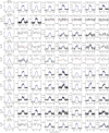 |
Fig. 1 Rotational lines observed with the IRAM 30m telescope in the 30 O-rich CSEs (black histograms). The blue lines indicate the calculated line profiles from the best-fit LVG model. The red lines correspond to the calculated line profiles with the maximum intensity compatible with the nondetection. |
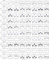 |
Fig. 1 continued. |
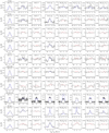 |
Fig. 1 continued. |
5.2 Modeling procedure
Here, we give a brief description of the model used to perform the non-LTE excitation and radiative transfer calculations (for details see Massalkhi et al. 2018). To derive accurate molecular abundances in each object, we take into account the specific physical properties for each envelope and source presented in Tables 1 and 2.
The main assumption in the model is that the CSE that surrounds the central AGB star has a smooth and spherically symmetric geometry that is produced by an isotropic mass loss with a constant mass loss rate Ṁ and a constant expansion velocity Vexp. We assume that the hydrogen in the CSE is molecular and its density structure (as a function of a distance r from the star) follows an r−2 law. The various physical quantities relating to the envelope such as the radial profiles of the gas density, gas temperature, and dust temperature, as well as the properties of the dust grains are described in Massalkhi et al. (2018). The only difference in this study is that we consider spherical grains of silicate with a radius of 0.1 μm, a mass density of 3.3 g cm−3, and optical properties for warm silicate from Suh (1999).
We chose to model the molecular line emission using the multishell large velocity gradient (LVG) method explained in more detail in Agúndez (2009) and Agúndez et al. (2012). The LVG formalism, first developed by Sobolev (1960), has been widely used to solve the molecular excitation and radiative transfer problem in environments with large velocity gradients. This approach is valid for molecular lines in circumstellar envelopes as long as they are not too optically thick. Bujarrabal & Alcolea (2013) showed thatthis formalism yields quite accurate excitation conditions even when the approximations of the method are marginally satisfied. These authors investigated the validity of the LVG formalism by studying the CO molecular excitation for different conditions and conclude that although the LVG approximation still produces good behavior in cases where the velocity gradient is low, the behavior is not as accurate for the very outer regions with high opacities. The LVG method provides a good compromise with respect to other methodologies such as Monte Carlo, which are more computationally expensive and exhibit problems of convergence when including a high number of energy levels.
Briefly, the CSE is divided into several concentric shells. The statistical equilibrium equations are then solved in each shell to determine the level populations. The radiation field which is needed to solve the statistical equilibrium equations is evaluated solving the radiative transfer under the LVG approximation. We assume that the molecules are excited by collisions with H2 molecules and He atoms and through radiation from three sources: the cosmic microwave background, the stellar radiation, and the thermal emission from dust. We also include infrared (IR) pumping to excited vibrational states for SiO, CS, and SiS. In the cases of SO and SO2, we only consider rotational levels within the ground vibrational state for simplicity and because of the less reliable collisional rate coefficients for ro-vibrational transitions.
5.3 Adopted abundance distribution
The abundance distribution is important in the radiative transfer modeling. For parent molecules that are injected from the inner parts of the envelope, the abundance may vary with radius due to two processes: condensation onto grains and photodissociation by ultraviolet (UV) photons. In reality, the abundance is expected to decrease from the thermochemical equilibrium (TE) value at the stellar surface in the dust formation region. The molecules are further depleted by the ambient radiation field which eventually determines the size of the emission envelope. Relating to this scenario, a few studies have reported on an abundance distribution to be consisting of two components, a compact high abundance in the inner regions of the CSE, and a lower abundance in the extended outer regions of the CSE (e.g., Schöier et al. 2007, Decin et al. 2010). For example, Schöier et al. (2004) modeled the SiO emission of the J = 6−5, J = 5−4, J = 3−2, and J = 2−1 lines in the CSE of the M-type star R Dor and found the need for a two-component abundance distribution which was characterized by a high abundance of 4 × 10⁻⁵ up to 1.2 × 1015 cm and a lower abundance of 3 × 10⁻⁶ at larger radii. This initial high abundance followed by a decrease was interpreted as adsorption of SiO onto dust. However, when Van de Sande et al. (2018) modeled the SiO emission with several low- and high-J transitions (up to J = 38−37) in the same object, R Dor, they found no indication of a two-component abundance distribution. Similarly, in the case of SiS, Schöier et al. (2007) modeled the emission in IK Tau and found a better fit to their observations when they included an inner component out to 1 × 1015 cm with a high SiS abundance of 2 × 10⁻⁵. However, Danilovich et al. (2019) performed sensitive ALMA observations with an angular resolution of ~ 150 mas that correponds to ~6 × 1014 cm and did not find evidence for such a jump in the abundance of SiS in the same source. Other studies reported on the molecular abundance distribution in CSEs as well. Agúndez et al. (2012) modeled lines of CS in the ν = 0−3 states in addition to several transitions of the isotopologues 13CS, C34 S, and C33 S in IRC +10216 and derived an abundance of 4 × 10⁻⁶ in the inner regions that decreased to 7 × 10⁻⁷ in the mid envelope at a radius of 2 × 1015 cm. Their result is in good agreement with that derived by Velilla-Prieto et al. (2019) that modeled the J = 2−1 lines of CS, and 13CS, C34 S, and C33 S using ALMA which also showed a decline in the abundance toward the intermediate envelope of IRC +10216 supporting a depletion scenario. However, no such abundance distribution is reported for the sulfur oxides thusfar that evidence any depletion (e.g., Danilovich et al. 2016, 2020).
Regardless whether or not these molecules experience a first abundance depletion due to dust condensation, they maintain a significant abundance in the extended outer envelope where photodissociation further removes the molecules from the gas phase. The lines observed in this study probe intermediate/outer regions of the envelope (see Sect. 6). That is, we are not sensitive to abundance gradients occurring in the inner envelope and the abundances derived are valid for the post-condensation region. We therefore adopt a simple scenario in which the fractional abundance remains constant throughout the envelope up to some region where it drops due to photodissociation. The adopted abundance radial distribution f(r) is described by a Gaussian as:
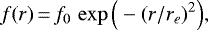 (1)
(1)
where f is the fractional abundance of the molecule relative to H2, f0 is the initial abundance, and re is the e-folding radius at which the abundance has dropped by a factor e. Danilovich et al. (2016) observed SO and SO2 emission in a sample of five stars O-rich CSEs, and found that SO2 has a Gaussian abundance distribution, whereas the SO abundance distribution differs between Gaussian for high mass-loss rate envelopes, and shell-like for low mass-loss rate envelopes where the abundance peaks at a distance from the central star. In their recent study on these two molecules using ALMA in two CSEs R Dor and IK Tau, Danilovich et al. (2020) found that SO and SO2 in R Dor have Gaussian distribution, while in IK Tau, SO and probably SO2 have a shell-like abundance distribution. Here, we adopt a Gaussian abundance distribution for all the molecules.
In their study on M-type stars, González Delgado et al. (2003) estimated the SiO emission size by using a scaling law that correlated re and the envelope density evaluated through the quantity Ṁ∕Vexp,
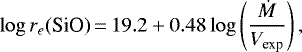 (2)
(2)
where re is given in cm, Ṁ in M⊙ yr−1, and Vexp in km s−1. We use Eq. (2) to determine the emission size of SiO, SiS, SO, and SO2 in our sample. The assumption of similar radial extents for SiO and SiS is discussed in our previous study of these molecules inC-rich CSEs in Massalkhi et al. (2019). Danilovich et al. (2018) derived empirical relations between re and Ṁ ∕Vexp for SiS and CS from a limited sample of M-, C-, and S-type stars which we noticed are unreliable outside the relatively narrow range of Ṁ ∕Vexp over which they were derived (for details see Massalkhi et al. 2019). In their recent study using ALMA data, Danilovich et al. (2020) found that SO and SO2 are colocated around the O-rich R Dor, with SO being slightly more extended than SO2. However, statistically robust empirical relations for the emission size of SO and SO2 have not been derived. Since the photodissociation rates of SO and SO2 under the interstellar radiation field are of the same order of that of SiO, a few times 10−9 s−1 (Heays et al. 2017; Agúndez et al. 2018), in the lack of better constraints on the emission size, we adopt the same radial extent for SiO, SiS, SO, and SO2. For CS, which has a significantly lower photodissociation rate than SiO, SO, and SO2, a few times 10−10 s−1 (Pattillo et al. 2018), we use a larger emission size as suggested by Massalkhi et al. (2019) for C-rich AGB stars and described by the following empirical relation:
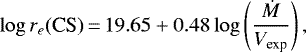 (3)
(3)
Briefly, we construct a physical model of the envelope for each source with the parameters given in Tables 1 and 2. Adopting the fractional abundance distributions given in the previous section, we perform excitation and radiative transfer calculations by varying the initial fractional abundance, f0, until the calculated line profiles match the observed ones. The criteria we adopted to determine how well the model fits the data is by matching the area of the calculated line to the observed one. The agreement between observed and calculated line area was better than 3% for the molecules for which we have only one line, SiO, CS, SiS, and SO, and better than 30% for SO2 because for this molecule we have four observed lines. When the line is undetected, we derive upper limits of the fractional abundance by choosing the maximum abundance that results in line intensities compatible with the noise level of the observations.
In our sample there are three sources which deserve to be considered separately, EP Aqr, X Her, and OH 26.5+0.6. We discuss the reasons and the procedure adopted for the line modeling of these sources in Sect. 5.4.
5.4 Peculiar sources
Some AGB stars are known to exhibit a double-component profile in some molecular lines like CO, with a narrow spectral feature centered on a much broader plateau, with both components having the same LSR velocity (Kahane & Jura 1996; Knapp et al. 1998; Kerschbaum & Olofsson 1999; Olofsson et al. 2002). The origin of these double-component profiles is still not clear. Knapp et al. (1998) suggested that it is an effect of episodic mass loss with highly varying gas expansion velocities that produces multiple shells where each shell has a different expansion velocity and different mass loss rate. Other studies argued that complicated geometries and kinematics play a role in the rise of the effect (Neri et al. 1998; Nakashima 2005; Castro-Carrizo et al. 2010; Kim & Taam 2012; Homan et al. 2015; Kim et al. 2019). Two of the sources that are known to exhibit this type of profile, X Her and Ep Aqr (Homan et al. 2018), are in our sample and their spectra are shown in Fig. 1. The two stars are M-type semiregular variable AGBs. From the rotational transitions observed here there is no sign of the superimposition of the narrow profile on the broader one in both sources. However, based on the observed line widths and expansion velocities it appears that the SiO line emission of X Her and EP Aqr are coming from the broad component, while the CS, SO and SO2 line emissions arise from the narrow component. The SiS rotational line is not detected in any of the sources, but in deriving abundance upper limits we assume that it behaves as CS, SO, and SO2 and arises from the narrow component. We then consider two different winds for the narrow and the broad component each with different values of the expansion velocity and the mass loss rate, as given in Table 2, and perform the radiative transfer andexcitation analysis independently.
Another source we encountered problems modeling is the extreme OH/IR AGB star OH 26.5+0.6. This star is thought to have gone through a superwind phase characterized by a dramatic increase of the mass loss rate (by a factor of ten at least) toward the end of the AGB (Iben & Renzini 1983) which ejects most of the remaining envelope and the initial mass of the star allowing the latter to evolve toward the planetary nebula phase. Justtanont et al. (1996) show evidence of two mass loss regimes: a higher density superwind that started recently (< 200 yr), and a lower density AGB wind that started earlier. From Justtanont et al. (1996), the reported gas mass loss rate for the superwind is Ṁ = 5.5 × 10⁻⁴ M⊙ yr−1 at r < 8.0 × 1015 cm and for the outer AGB wind is Ṁ = 1 × 10⁻⁶ M⊙ yr−1 at greater radii. Moreover, we adopt the gas kinetic temperature profile for the object reported by the authors as well (solid line in Fig. 7b of Justtanont et al. 1996). After setting the density and temperature structure in the envelope, we model the rotational line emission of the molecules.
6 Results from line modeling
The calculated line profiles from our best-fit LVG model for each of the sources are shown in blue in Fig. 1, where they are compared with the observed line profiles (black histograms). In those cases in which the lines are not detected, the calculated line profile is plotted in red instead.
In general, the calculated line shapes agree well with the observed ones. However, there are profiles that exhibit complexities which our model is not able to reproduce, for example, the SO2 emission in IK Tau. This is probably due to the simplicity of our approximated physical model which assumes smooth and spherically symmetric envelopes and does not take into consideration any deviations from that. In the case of the SiO J = 3−2 line, the observed profiles are mostly parabolic or triangular, although for some sources, such as RR Aql, the model produces flat-topped shapes. The assumption of a constant expansion velocity in our model could be playing a factor in the discrepency between the calculated and the observed line profile since as mentioned previously triangular line profiles probably indicate emission from accelerating regions close to the star. Another explanation could be related to the line opacity τ. In these cases, the line opacity is probably around one, with the modeled line having τ slightly below one and the observed line having τ slightly above one. In any case, the overall agreement between calculated and observed line profiles is good.
The excitation and radiative transfer calculations give us information about the excitation and emission region of the molecules in the envelope. In regards to the emission region, the model indicates that most of the contribution to the line emission of the five molecules is coming from regions 1015 −1016 cm from the star, i.e, most of the emission arises from intermediate and outer regions of the envelope, rather than from the inner regions. To evaluate the role of IR pumping to vibrationally excited states for SiO, CS, and SiS, we ran models excluding IR pumping. Our calculations indicate that in the absence of IR pumping, the emission is more compact than when IR pumping is included. The calculations also show that IR pumping has an effect on the intensities of the observed lines of SiO, CS and SiS. Neglecting IR pumping results in a systematic decrease in the integrated line intensities of ~ 40% for SiO J = 3−2, ~ 50% for CS J = 3−2, and ~ 35% for SiS J = 8−7.
In regards to the excitation of the rotational levels, the model indicates that the rotational levels of the five studied molecules are thermalized in the warm and dense inner layers of the envelopes. However, as the radial distance from the star increases and the gas density decreases, the rotational levels become suprathermally populated (with the ratio of the excitation temperature, Tex, to the kinetic temperature, Tk, greater than unity, Tex /Tk > 1) for SiS, CS, SO and SO2 in the regions where most of the emission is coming from. For SiO, the population of rotational levels vary. Mostly, they are subthermally populated (Tex/Tk < 1), however for a few envelopes (e.g., RR Aql, NV Aur, WX PSc), the levels are suprathermally populated. The behavior for SiO, CS, and SiS, is largely caused by IR pumping. In comparison, in C-rich CSEs, IR pumping causes the rotational transitions of these molecules to be all suprathermally excited (Massalkhi et al. 2019). We can conclude that IR pumping plays an important role in the excitation of the rotational emission of SiO, CS, and SiS whether in C-rich or O-rich envelopes.
7 Discussion
The fractional abundances relative to H2, f0, derived for SiO, CS, SiS, SO,and SO2 in the 30 O-rich envelopes are presented in Table 4 and are shown as a function of the envelope density proxy, Ṁ ∕Vexp, in blue in Fig. 2. In the panels of SiO, CS, and SiS we also include (plotted in red) the fractional abundances derived in a sample of 25 C-rich envelopes by Massalkhi et al. (2019).
7.1 Fractional abundances derived
7.1.1 SiO
The SiO fractional abundances f0(SiO) derived in this study for the 30 O-rich AGB stars are presented in blue in the upper middle panel of Fig. 2. We overplot in red the SiO abundances derived by Massalkhi et al. (2019) for 25 C-rich AGB stars.
One of the first comprehensive studies of molecular abundances in circumstellar envelopes was done by González Delgado et al. (2003), who focused on SiO in a large sample of about 40 O-rich CSEs. They used multiline data to determine the size of the emittingregion and the SiO abundance simultaneously. We share 21 objects with these authors. In general, our derived SiO abundances are very similar to theirs.
From Fig. 2, we notice from the SiO fractional abundances we are not able to distinguish the chemical type, either O-rich (in blue) or C-rich (in red). Schöier et al. (2006a) found the same result when comparing the distribution of their derived SiO abundances in C-rich stars to the distribution of SiO abundances in M-type stars derived by González Delgado et al. (2003). That is, observations indicate that the SiO abundance does not depend on the C/O ratio at the stellar surface. The mean fractional abundance of SiO we obtain is similar in both types of CSEs, with log f0(SiO) = −5.5 ± 0.7 in O-rich CSEs and logf0(SiO) = − 5.8 ± 0.6 in C-rich CSEs7.
The fact that the SiO abundance injected into the expanding wind is not sensitive to the C/O ratio is in line with theoretical expectations. Thermochemical equilibrium calculations predict that SiO maintains a uniform and high fractional abundance of several 10−5 from the photosphere out to 10 R⋆ in O-rich CSEs, while in C-rich CSEs the predicted fractional abundance from 5 R⋆ is also on the order of 10−5. The main difference occurs in the innermost region, from the photosphere to around 5 R⋆, where SiO has a low abundance in C-rich conditions while it maintains a high abundance in O-rich CSEs (Agúndez & Cernicharo 2006; Agúndez et al. 2020). In a scenario of chemical equilibrium, it seems that the low SiO abundance within 5 R⋆ in C-rich CSEs does not have an influence on the final SiO abundance that is injected into the expanding wind, and that chemical equilibrium holds for SiO in the high abundance region located beyond 5 R⋆. The low SiO abundance predicted by chemical equilibrium in the innermost envelope has been inferred by modeling multiwavelength observations of the carbon star IRC +10216 by Schöier et al. (2006b). The nonequilibrium scenario of shocks induced by the stellar pulsation of Cherchneff (2006) also predicts a low sensitivity of the SiO abundance on the photospheric C/O ratio. In the model of Cherchneff (2006), for C/O < 1 shocks have a very limited effect on the SiO fractional abundance in the inner part of the wind as it stays around ~ 10−5 from the photosphere out to 5 R⋆. For C/O > 1, the authors find that the low chemical equilibrium abundance of ~10−8 is enhanced rapidly to values around 10−5 in the 1–5 R⋆ region. Therefore, the SiO abundances calculated at 5 R⋆, which are supposed to be the ones injected into the expanding wind, are of the same order in O-rich and C-rich stars. In summary, theoretical studies show that the SiO abundance has no apparent dependence on the C/O ratio in the outer wind which is in agreement with the findings from our observational study. The different behavior of the SiO abundance in the inner wind as predicted by theoretical studies probably explains why strong SiO maser emission is detected toward O-rich stars and not toward carbon stars (e.g., Pardo et al. 2004; Cotton et al. 2004). In view of the high SiO abundance observed in C-rich stars, this could suggest that the SiO molecules are formed further out in the wind in C-rich envelopes where the physical conditions are not likely to allow the pumping by IR photons, and thus the inversion of SiO level populations.
The fractional abundance of SiO in the O-rich sample varies substantially from as low as 7.0 × 10⁻⁸ up to 4.5 × 10⁻⁵. This variation in the SiO abundance as illustrated in Fig. 2, whether C-rich or O-rich, shows a clear trend in which SiO becomes less abundant as the density in the wind, Ṁ ∕Vexp, increases. Schöier et al. (2006a) and Massalkhi et al. (2019) presented analysis of circumstellar SiO abundances for carbon stars, and González Delgado et al. (2003) for M-type stars and likewise they find a similar behavior of a strong anticorrelation between the abundance and the wind density which was interpreted as an effect of increased adsorption of SiO onto dust grains at high densities. Here, we confirm the results found for O-rich stars by González Delgado et al. (2003). We found a similar trend when we investigated SiC2 in a sample of 25 carbon-rich AGB stars (see upper left panel in Fig. 2 for comparison), which was interpreted as that SiC2 is being efficiently incorporated into dust grains and playing an important role in the formation of silicon carbide dust in C-rich envelopes (Massalkhi et al. 2018). Adsorption of SiO onto dust grains in O-rich envelopes is predicted theoretically by chemical kinetics models (Van de Sande et al. 2019). We note that the median fractional abundance of SiO of the Mira-type variables, 2.5 × 10⁻⁶, is lower by a factor of 6 with respect to the median value of the semiregular variables, 1.5 × 10⁻⁵, which may be related to the mass loss rate rather than the stellar variability type. González Delgado et al. (2003) found a similar result where the high mass-loss rate Miras in their sample have a median abundance that is more than six times lower than that of the irregular and semiregular variables.
Silicates are known to be one of the most important types of dust in oxygen-rich envelopes and SiO has long been discussed to be the gas-phase precursor of silicate dust, mainly because of its high abundance in O-rich envelopes. The trend that we see here between the fractional abundance and the wind density supports this hypothesis.
Fractional abundances of SiO, CS, SiS, SO, and SO2 derived.
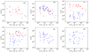 |
Fig. 2 Results for the radiative transfer and excitation analysis toward the sample of AGB stars. Fractional abundance f0 derived for SiC2 obtained byMassalkhi et al. (2018) for C-rich AGB stars (upper left), fractional abundance for SiO (upper middle), fractional abundance for CS (upper right), and fractional abundance for SiS (lower left) as a function of density measure Ṁ ∕Vexp for oxygen stars (blue) and carbon stars (red; Massalkhi et al. 2019). Fractional abundance for SO (lower middle) and for SO2 (lower right)in O-rich envelopes as a function of density measure Ṁ∕Vexp. Downward arrows represent upper limits to f0. |
7.1.2 CS
The fractional abundances derived for CS in the O-rich envelopes are shown in blue as a function of Ṁ ∕Vexp in the upper right panel of Fig. 2. We also show in red the CS fractional abundances derived for the 25 C-rich AGB stars studied in Massalkhi et al. (2019).
Bujarrabal et al. (1994) searched for CS J = 3−2 and J = 5−4 transitions in a large sample of evolved stars. Their sample contains 17 O-rich stars, 10 of which are in our sample. These authors derived abundances using a simple analytical expression based on the integrated intensities of the observed lines and assumes a constant fractional abundance inside a given radius. In general, their CS abundances are higher than ours with varying degrees, for example, ranging from a factor of two for some sources, like V1300 Aql, to one order of magnitude for other sources, like IK Tau, to a highest factor of 47 for RX Boo, where our value is an upper limit. These authors remark that their approach holds for optically thin lines and estimated only a lower limit if the line was optically thick. Danilovich et al. (2018) surveyed a diverse sample of AGB stars. They detected CS in only the highest mass loss rate O-rich stars and derived CS abundances in agreement with ours for some sources, such as GX Mon and V1300 Aql, while for other sources their derived values were approximately an order of magnitude higher than ours, such as IK Tau and RR Aql, the latter being an upper limit in both studies.
Comparing the values of f0(CS) in oxygen-rich and carbon-rich envelopes in Fig. 2, the derived abundances show substantial variations between the two chemical types where the mean fractional abundance for O-rich CSEs is log f0(CS) = −8.0 ± 0.6, more than two orders of magnitude lower than for C-rich CSEs, log f0(CS) = −5.4 ± 0.5. It is clear that the formation of CS is dependent on the photospheric C/O ratio of the star. We also notice that CS is mostly detected in O-rich CSEs with high mass-loss rates, while in C-rich CSEs, CS is detected in all the sources of the sample, regardless of the mass loss rate. Carbon monosulfide forms more readily in C-rich environments since there is available carbon, that is, not trapped by CO, to form C-bearing molecules. On the other hand, the formation of CS in O-rich CSEs is more surprising as all the available carbon is expected to be locked up in CO.
Chemical equilibrium calculations predict negligible abundances for CS in O-rich CSEs, more than 3–4 orders of magnitude below the observed values (Agúndez et al. 2020). It is clear that some nonequilibrium process is enhancing the abundance of CS in O-rich envelopes. A possible explanation for the synthesis of this molecule could be related to photochemistry in a clumpy CSE, as investigated by Agúndez et al. (2010). In this scenario, interstellar UV photons penetrate into the inner regions of the envelope, break the CO bond and induce changes in the chemical composition which ultimately allow for the formation of CS and other C-bearing molecules. Their calculations predict abundances of ~ 10−9−10−8 for mass-loss rates in the 10−7–10−5 M⊙ yr−1, in agreement with the abundances we find here. Similar models by Van de Sande et al. (2018) examined the effects that clumping and porosity have on the chemistry in the AGB outflow and found slightly higher peak abundances of ~ 10−7. However, in their recently published corrigendum these authors no longer find this peak, instead the fractional abundance of CS drop to ~10−10 (Van de Sande et al. 2020). Another explanation for the formation of CS in O-rich environments could be related to the variable nature of AGB stars. Periodic shock waves caused by stellar pulsations propagate through the photosphere and alter the gas chemistry where the collisional destruction of CO in the shocks could release free atomic carbon and trigger the formation of CS in O-rich environments (Duari et al. 1999; Cherchneff 2006; Gobrecht et al. 2016). The shock-induced chemistry model of Cherchneff (2006) predicts that CS reaches abundances of a few times 10−6 in envelopes with C/O < 1, that is to say, significantly above the mean abundance derived here from observations.
To investigate the reason for the nondetection of CS in the low mass loss rate objects, we consider the variability type (Mira variable andsemiregular variable, see Table 4) of the O-rich stars. The type of variability is generally attributed to the pulsation of the star and therefore could influence the shock conditions and provide an explanation of the abundance differentiation between high- and low-mass loss rate O-rich stars. However, we see no indication of a dependence between the abundance of CS and the variability type. On one hand, the nondetection of CS in these envelopes could be due to a low fractional abundance of the molecule, on the other hand, it could be due to a lack of sensitivity.
The CS fractional abundance in the O-rich sample varies by about two orders of magnitude, ranging from as low as 1 × 10⁻⁹ to as high as 1.1 × 10⁻⁷, yet unlike the case of SiO, this variation shows no apparent trend that the CS abundance decreases as the density in the wind (Ṁ ∕Vexp) increases for O-rich envelopes. Such a trend is however evident for carbon-rich envelopes. This suggests that CS molecules are more likely to adsorb onto dust grains in C-rich CSEs than in O-rich ones. While CS is thought to play a role in the formation of MgS dust in C-rich envelopes (Massalkhi et al. 2019), in the case of O-rich envelopes CS does not seem to be affected by adsorption onto dust grains and to be playing a role in the formation of dust.
7.1.3 SiS
In the lower left panel of Fig. 2 we show as a function of Ṁ ∕Vexp the fractional abundances of SiS derived in the 30 O-rich envelopes studied here (in blue) and in the 25 C-rich envelopes studied by Massalkhi et al. (2019; in red).
Schöier et al. (2007) reported on the detection of SiS line emission in 8 oxygen-rich envelopes, all of which are included in our sample. They performed radiative transfer calculations to derive abundances adopting, similarly to us, an abundance distribution based on the scaling law established by González Delgado et al. (2003) for SiO in M-type stars. Our SiS abundances are in good agreement with theirs for all of the sources.
By looking to the fractional abundances f0 (SiS) derived in the O-rich sample (see Table 4) we notice that they vary considerably among different sources, between < 4.0 × 10⁻⁹ and 1.9 × 10⁻⁶. The mean fractional abundance in the O-rich sample is log f0(SiS) = −7.0 ± 0.7, while in C-rich AGB stars is log f0(SiS) = −5.5 ± 0.4, that is, an order of magnitude higher than in O-rich envelopes. Similarly, in their study of SiS in a small sample of oxygen- and carbon-rich envelopes, Schöier et al. (2007) found SiS abundances in carbon-rich envelopes about an order of magnitude higher than in oxygen-rich envelopes. This indicates that SiS has a marked chemical differentiation based on the photospheric C/O ratio, being more preferentially formed in C-rich environments than in O-rich ones.
According to chemical equilibrium, in C-rich envelopes SiS reaches a high fractional abundance of about 10−5 from 2 R⋆, while in O-rich envelopes the abundance of SiS is low in the very inner regions but rises to values slightly below 10−5 from 2 R⋆ beyond 5 R⋆ (Agúndez et al. 2020). That is, the differentiation between C-rich and O-rich is restricted to the very inner regions, but beyond 5 R⋆ SiS is predicted to reach high abundances, on the order of 10−5, in both C- and O-rich envelopes. The low SiS abundances observed here in some O-rich envelopes are thus not expected according to chemical equilibrium. On the other hand, nonequilibrium chemical models based on shocks induced by the stellar pulsation predict a dependence of the SiS abundance on the C/O ratio, with abundances on the order of 10−5 and 10−8 at 5 R⋆ in the inner regions of C- and O-rich, respectively, envelopes (Cherchneff 2006). The SiS abundances derived from observations here agree with the predictions of these models in terms of differentiation based on the C/O ratio, although there is a discrepancy because some of our observed abundances are significantly above those predicted by the model. For example, Cherchneff (2006) predicts an SiS fractional abundance for TX Cam of ~ 10−8 at 5 R⋆, while for this source we derive an abundance of 3.9 × 10⁻⁷. Therefore, chemical equilibrium overestimates the SiS abundances in O-rich envelopes while nonequilibrium models underestimate them.
Strikingly, we noticed that SiS is not detected in envelopes with low mass loss rates < 10−6, while it is detected in all sources above this threshold. This fact has been reported by some previous observational studies (Bujarrabal et al. 1994; Danilovich et al. 2015, 2018; Massalkhi et al. 2019). Massalkhi et al. (2019) surveyed a sample of 25 C-rich AGB stars in SiS J = 8−7 and J = 7−6 emission and did not detect emission below the same threshold as well. They speculated that the nondetection of SiS in the low mass-loss rate C-rich envelopes could be either caused by a lack of the constituent elements, which would be trapped in other S- and Si-bearing molecules like SiO, SiC2, and CS, or could be due to sensitivity which might be the case here as well. Danilovich et al. (2019) discussed based on previous studies that SiS does not form readily in low-mass loss rate semi-regular variables, where the molecule otherwise reaches higher abundunces in Mira variable type CSEs. However, these authors detect faint SiS J = 19−18 emission toward the low mass-loss rate semiregular variable, R Dor, using ALMA and derive an abundance of 1.5 × 10⁻⁸ which indicates that the nondetection of SiS in low mass loss rate semiregular variables could be due to low sensitivity. In this study, we do not detect SiS in low-mass loss rate objects of both, semiregular and Mira variables, that is to say, we do not see a dependence of the SiS fractional abundance on the variability type, similar to the case of CS.
While SiS shows a tentative trend of a decreasing abundance with increasing envelope density for C-rich CSEs (Massalkhi et al. 2019), which was interpreted in terms of adsorption onto dust grains, here we do not see any similar trend, implying that SiS is probably not an important gas-phase precursor of dust in O-rich CSEs. However, chemical kinetics models by Van de Sande et al. (2019) predict adsorption of SiS onto dust grains in O-rich outflows.
7.1.4 SO
The resulting SO fractional abundances are shown as a function of Ṁ ∕Vexp in the lower middle panel of Fig. 2. Systematic studies of the abundance of SO on large samples of AGB stars are scarce. In fact, for some of the sources in our sample, SO abundances are reported for the first time. One of those studies was made by Bujarrabal et al. (1994), who surveyed a large sample of evolved stars in several molecular lines, including SO 65 −54. Their sample contains 18 O-rich objects, 11 of which are in our sample. For some sources, our derived abundances are higher than theirs, and for other sources, the opposite is found. But in general the difference is within a factor of a few. The modeling performed by these authors is based on a somewhat simple method as mentioned previously, in which an analytical expression is used to derive the abundance of the molecules. A more complex abundance derivation based on radiative transfer modeling was done by Danilovich et al. (2016) using high- and low-Eu lines of SO (and SO2; see below) in a small sample of five M-type AGB stars, four of which are in our sample. The authors find that the spatial distribution of SO differs between the low mass loss rate objects (R Dor, and W Hya) and the high mass loss rate ones (IK Tau, R Cas, and TX Cam), where the former were best reproduced by a Gaussian disribution whereas the latter by a shell-like one. For the four sources we have in common, their derived abundances are higher than ours by a factor of a few. In their recent study of two O-rich envelopes using ALMA, Danilovich et al. (2020) confirmed their previous findings in that the SO abundance distribution in IK Tau is shell-like with a constant inner abundance of 4.1 × 10⁻⁷, not very different from the value derived in this study (1.7 × 10⁻⁷), that increases to 2.2 × 10⁻⁶ at 5 × 1015 cm followed by a decline at e−folding radius 1.3 × 1016 cm. Velilla Prieto et al. (2017) also surveyed IK Tau and derived f0(SO) ≥ 8 × 10⁻⁶, which is significantly higher than the value derived here (1.7 × 10⁻⁷). These authors discuss that their derived SO abundance for this source may be overestimated since it is higher than previous observational studies and higher than abundances predicted by chemical equilibrium models, and that the reason behind this discrepancy is the uncertainty in the adopted SO emitting region.
The values of f0(SO) range between <6.8 × 10⁻⁸ and 6 × 10⁻⁶ and have a mean fractional abundance of log f0(SO) = −6.1 ± 0.6. Chemical equilibrium calculations predict a peak SO abundance in the 1–10 R⋆ region of ~ 10−7 (Agúndez et al. 2020), while nonequilibrium chemical models considering shocks induced by the pulsation of the star predict similar abundances at 5 R⋆ (Cherchneff 2006). Therefore, on average, our observed SO abundances are higher than theoretical predictions of the inner wind. For SO, we see no dependence of the fractional abundance on the stellar variability type.
The distribution of the fractional abundances derived in the O-rich sample show hints of decreasing SO abundance with increasing density. This is however tentative as it is not as evident as in the case of SiO. Danilovich et al. (2016) found a similar trend of SO being less abundant with wind density, although this result was based on a reduced sample of only 3 objects (TX Cam, IK Tau, and R Cas) with a limited range of mass loss rates. If the tentative decrease in the abundance of SO with increasing envelope density that we see here is interpreted in terms of adsorption onto dust grains, SO could emerge as a candidate togas-phase precursor of dust. To date, no sulfur-containing condensate has been identified in the spectra of O-rich envelopes, although CaS and FeS are expected to be important solid carriers of sulfur in these environments (Lodders & Fegley 1999; Agúndez et al. 2020).
7.1.5 SO2
The fractional abundances derived for SO2 are shown asa function of Ṁ∕Vexp in the lowerright panel of Fig. 2. For some of the sources in our sample, SO2 abundances are reported for the first time.
Infrared observations, in particular, the ISO/SWS detection of the 7.3 μm ν3 band in a few AGB stars by Yamamura et al. (1999) and observations of high energy rotational lines by, e.g., Danilovich et al. (2016) and Velilla Prieto et al. (2017) indicate that SO2 is formed in the inner layers of the CSE. Omont et al. (1993) surveyed a diverse sample of evolved stars in sulfur-bearing molecules and derived SO2 abundances for 7 of the objects in our sample. For some sources, the abundances derived by these authors are similar to the values derived in this work. While for other sources, the derived abundances are different, like RX Boo, their value is 50 times higher than ours. These authors used a relatively simple method for estimating the molecular abundances, which is based on an analytical expression in which they assumed a constant excitation temperature for simplicity. A study was conducted by Danilovich et al. (2016) to investigate the SO2 rotational lines observed with Herschel/HIFI in addition to further archival data toward a small sample M-type AGB stars. They performed radiative transfer modeling and derived SO2 abundance toward three of the objects that are in our sample, IK Tau, W Hya, and R Cas. They find SO2 fractional abundance in IK Tau similar to ours assuming a Gaussian distribution. They note that their SO2 model for IK Tau is uncertain due to the difficulty of determining an abundance distribution. In fact, in their recent study using ALMA, these authors suspect that the SO2 abundance in IK Tau is consistent with a shell-like distribution and not a Gaussian distribution (Danilovich et al. 2020). For W Hya and R Cas, their derived abundances are higher than ours, by a factor of 50 (with ours being an upper limit) and an order of magnitude, respectively. They also note that their SO2 model for R Cas is very uncertain due to the fact that they had only two detected lines toward that source. The mean fractional abundance of SO2 in the 30 O-rich envelopes studied here is log f0(SO2) = −6.2 ± 0.7, that is, very similar to that of SO.
Sulfur dioxide is predicted to have low abundances (< 10−10), well below the observed values, in the inner regions of O-rich envelopes according to chemical equilibrium (Agúndez et al. 2020). There must be a nonequilibrium process that enhances the formation of SO2 in the inner envelope. The shock-induced chemistry scenario of Cherchneff (2006) also predicts very low abundances (10−13–10−12) for SO2 in the inner winds of O-rich AGB stars. Clearly, observations and theory maintain a severe discrepancy with respect to the abundance of SO2 in the innerenvelope of M-type stars. Similar to SO, we see no dependence of the SO2 fractional abundance on the stellar variability type.
In their study on sulfur molecules in M-type AGB stars, Danilovich et al. (2016) reported that SO and SO2 are the main reservoirs of sulfur in the inner regions of the CSE of W Hya and R Cas, with more uncertainties for the latter. For W Hya, they derived a combined fractional abundance of SO and SO2 of ~ 10−5 within the inner layers of the wind, thus accounting for most of the sulfur. Here in this work, the combined fractional abundance of CS, SiS, SO, and SO2 in the intermediate regions of the W Hya envelope is just ~8 × 10⁻⁷, well below the elemental abundance of S. This could point to depletion of sulfur through dust condensation in this object. A large fraction of the sulfur could also be trapped as gaseous H2 S, which is abundant in O-rich CSEs (Danilovich et al. 2017). In any case, for SO2 we do not see any clear trend of decreasing f0 (SO2) with increasing envelope density that could point to this molecule as a gas-phase precursor of dust in O-rich envelopes.
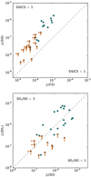 |
Fig. 3 Comparison of abundances between different pairs of molecules. The derived fractional abundances relative to H2 of CS vs. SiS (upper panel) and SO vs. SO2 (lower panel). Those sources with nondetections are denoted with arrows. The diagonal dashed lines indicate where the abundances of the two molecules become equal.The orange circles indicate fractional abundances with an upper limit. |
7.2 Correlations between abundances of different molecules
In Fig. 3 we plot the derived fractional abundance of CS against that of SiS (upper panel) and the fractional abundance of SO against that of SO2 (lower panel). We find that SiS is systematically more abundant than CS in the 30 O-rich envelopes studied, as indicated by the fact that all sources lie in the region ofSiS/CS >1, apart from EP Aqr that falls on the dashed line representing equal amounts of SiS and CS. Similarly, Danilovich et al. (2018) determined the CS and SiS abundances in a sample of AGB stars, and found SiS to be systematically more abundant than CS in their O-rich sample. Therefore, SiS seems to be a more abundant gas-phase reservoir of sulfur than CS in oxygen star envelopes. The behavior is thus different to that of C-rich envelopes, where CS and SiS have comparable abundances (Massalkhi et al. 2019). Moving on to the lower panel in Fig. 3, the comparison of SO and SO2 shows that in some sources SO is more abundant, like in R LMi and BK Vir, while in other sources SO2 is more abundant, like in NV Aur and V1111 Oph. In general, the data points fall along the line defined by f0 (SO) = f0(SO2) and there is no clear preference for either the SO/SO2 > 1 or the SO/SO2 < 1 sides. By looking to those sources where both SO andSO2 are detected, it seems that in oxygen-rich envelopes, SO and SO2 have abundances of the same order, carrying similar amounts of sulfur.
Regardless of which pair of molecules from those shown in Fig. 3, in both cases there is a trend in which the higher the abundance of one molecule the more abundant the other is, ie., the abundances of SO and SO2, and of SiS and CS, seem to scale with each other which suggests a chemical connection between the members of each couple of molecules. Danilovich et al. (2018) found this type of correlation for CS and SiS in a sample including C-, M-, and S-type stars, although in that study the trend is considered tentative because of the small number of sources included. Massalkhi et al. (2019) also found a similar correlation between the three molecules CS, SiO, and SiS in their large sample of C-rich CSEs. We remark, however, that the trends in Fig. 3 become less robust given the upper limits on some of the fractional abundances in the sources where these molecules are not detected.
8 Conclusion
In this study we observed SiO, CS, SiS, SO, and SO2 using the IRAM 30m telescope in a statistically meaningful sample of 30 O-rich AGB stars covering a wide range of mass-loss rates and circumstellar properties. We performed an extensive radiative transfer and excitation analysis based on the LVG method to derive the fractional abundance of these molecules in the circumstellar envelopes.
We found that the derived circumstellar abundances of SiS and CS have a clear dependence on the photospheric C/O ratio of the star, while SiO is not sensitive to it. Moreover, the fractional abundance of CS and SiS in carbon-rich CSEs are about two and one orders of magnitude, respectively, higher than in oxygen-rich envelopes, whereas the fractional abundance of SiO in both chemical types is of the same order of magnitude. Chemical equilibrium correctly predicts that SiO is abundant and that SiS and SO can reach high abundances in O-rich stars. However, the observed abundances of CS and SO2 are higher than predicted by several orders of magnitude. Nonequilibrium chemical models succeed to different extents in reproducing the observed abundances. A scenario of photochemistry in a clumpy envelope accounts for the abundance enhancement of CS. On the other hand, a scenario of shocks induced by the stellar pulsation results in abundances that are 1–3 orders of magnitude too high for CS, somewhat lower than observed for SiS and SO, and well below the observed values for SO2.
We find that the abundances of SiS and CS, on one hand, and SO and SO2, on the other, are positively correlated which suggests a chemical connection between the members of each couple. Moreover, as already found for C-rich envelopes, we find a clear trend of decreasing SiO abundance with increasing envelope density in O-rich envelopes, which points to adsorption of SiO onto dust grains. A similar trend is observed for SO, although not as clear as for SiO. Therefore, SiO and SO are likely candidates to act as gas-phase precursors of dust in O-rich envelopes. In the cases of CS, SiS, and SO2, abundances span over 2–3 orders of magnitude with no obvious correlation with the envelope density. These three molecules are thus less attractive candidates to be precursors of dust.
Our conclusions on the role of these molecules as gas-phase precursors of dust are based on low energy rotational lines, which probe post-condensation regions. More observations, in particular high-J lines and interferometric observationsprobing the inner regions of the envelopes, are needed to affirm the conclusions obtained in this study.
Acknowledgements
We thank the IRAM 30m staff for their help during the observations. This research has made use of the SIMBAD database, operated at CDS, Strasbourg, France. We acknowledge funding support from the European Research Council (ERC Grant610256: NANOCOSMOS) and from Spanish MINECO through grant AYA2016-75066-C2-1-P. M.A. thanks Spanish MINECO for funding support through the Ramón y Cajal programme (RyC-2014-16277). L.V.P. acknowledges funding support from the Swedish Research Council and the European Research Council (ERC Consolidator Grant 614264).
Appendix A Observed lines
Observed line parameters.
References
- Agúndez, M. 2009, PhD thesis, Universidad Autónoma de Madrid, Spain [Google Scholar]
- Agúndez, M., & Cernicharo, J. 2006, ApJ, 650, 374 [NASA ADS] [CrossRef] [Google Scholar]
- Agúndez, M., Cernicharo, J., & Guélin, M. 2010, ApJ, 724, L133 [NASA ADS] [CrossRef] [Google Scholar]
- Agúndez, M., Fonfría, J. P., Cernicharo, J., et al. 2012, A&A, 543, A48 [NASA ADS] [CrossRef] [EDP Sciences] [Google Scholar]
- Agúndez, M., Roueff, E., Le Petit, F., & Le Bourlot, J. 2018, A&A, 616, A19 [NASA ADS] [CrossRef] [EDP Sciences] [Google Scholar]
- Agúndez, M., Martínez, J. I., de Andres, P. L., Cernicharo, J., & Martín-Gago, J. A. 2020, A&A, 637, A59 [CrossRef] [EDP Sciences] [Google Scholar]
- Balança, C., & Dayou, F. 2017, MNRAS, 469, 1673 [NASA ADS] [CrossRef] [Google Scholar]
- Balança, C., Spielfiedel, A., & Feautrier, N. 2016, MNRAS, 460, 3766 [NASA ADS] [CrossRef] [Google Scholar]
- Balança, C., Dayou, F., Faure, A., Wiesenfeld, L., & Feautrier, N. 2018, MNRAS, 479, 2692 [CrossRef] [Google Scholar]
- Banerjee, D. P. K., Varricatt, W. P., Mathew, B., Launila, O., & Ashok, N. M. 2012, ApJ, 753, L20 [NASA ADS] [CrossRef] [Google Scholar]
- Bogey, M., Civiš, S., Delcroix, B., et al. 1997, J. Mol. Spectrosc., 182, 85 [NASA ADS] [CrossRef] [Google Scholar]
- Bujarrabal, V., & Alcolea, J. 2013, A&A, 552, A116 [NASA ADS] [CrossRef] [EDP Sciences] [Google Scholar]
- Bujarrabal, V., Fuente, A., & Omont, A. 1994, A&A, 285, 247 [NASA ADS] [Google Scholar]
- Castro-Carrizo, A., Quintana-Lacaci, G., Neri, R., et al. 2010, A&A, 523, A59 [NASA ADS] [CrossRef] [EDP Sciences] [Google Scholar]
- Cernicharo, J. 1985, IRAM Internal Rep. 52 [Google Scholar]
- Cernicharo, J., Spielfiedel, A., Balança, C., et al. 2011, A&A, 531, A103 [NASA ADS] [CrossRef] [EDP Sciences] [Google Scholar]
- Chandra, S., Kegel, W. H., Le Roy, R. J., & Hertenstein, T. 1995, A&AS, 114, 175 [NASA ADS] [Google Scholar]
- Cherchneff, I. 2006, A&A, 456, 1001 [NASA ADS] [CrossRef] [EDP Sciences] [Google Scholar]
- Chiavassa, A., Freytag, B., & Schultheis, M. 2018, A&A, 617, L1 [NASA ADS] [CrossRef] [EDP Sciences] [Google Scholar]
- Cotton, W. D., Mennesson, B., Diamond, P. J., et al. 2004, A&A, 414, 275 [NASA ADS] [CrossRef] [EDP Sciences] [Google Scholar]
- Danilovich, T., Teyssier, D., Justtanont, K., et al. 2015, A&A, 581, A60 [NASA ADS] [CrossRef] [EDP Sciences] [Google Scholar]
- Danilovich, T., De Beck, E., Black, J. H., Olofsson, H., & Justtanont, K. 2016, A&A, 588, A119 [NASA ADS] [CrossRef] [EDP Sciences] [Google Scholar]
- Danilovich, T., Van de Sande, M., De Beck, E., et al. 2017, A&A, 606, A124 [NASA ADS] [CrossRef] [EDP Sciences] [Google Scholar]
- Danilovich, T., Ramstedt, S., Gobrecht, D., et al. 2018, A&A, 617, A132 [Google Scholar]
- Danilovich, T., Richards, A. M. S., Karakas, A. I., et al. 2019, MNRAS, 484, 494 [NASA ADS] [CrossRef] [Google Scholar]
- Danilovich, T., Richards, A. M. S., Decin, L., Van de Sand, M., & Gottlieb, C. A. 2020, MNRAS, 494, 1323 [CrossRef] [Google Scholar]
- Dayou, F., & Balança, C. 2006, A&A, 459, 297 [NASA ADS] [CrossRef] [EDP Sciences] [Google Scholar]
- De Beck, E., Decin, L., de Koter, A., et al. 2010, A&A, 523, A18 [NASA ADS] [CrossRef] [EDP Sciences] [Google Scholar]
- De Beck, E., Decin, L., Ramstedt, S., et al. 2017, A&A, 598, A53 [NASA ADS] [CrossRef] [EDP Sciences] [Google Scholar]
- Decin, L., De Beck, E., Brünken, S., et al. 2010, A&A, 516, A69 [NASA ADS] [CrossRef] [EDP Sciences] [Google Scholar]
- Decin, L., Richards, A. M. S., Waters, L. B. F. M., et al. 2017, A&A, 608, A55 [NASA ADS] [CrossRef] [EDP Sciences] [Google Scholar]
- Denis-Alpizar, O., Stoecklin, T., Guilloteau, S., & Dutrey, A. 2018, MNRAS, 478, 1811 [NASA ADS] [CrossRef] [Google Scholar]
- Dharmawardena, T. E., Kemper, F., Scicluna, P., et al. 2018, MNRAS, 479, 536 [NASA ADS] [Google Scholar]
- Díaz-Luis, J. J., Alcolea, J., Bujarrabal, V., et al. 2019, A&A, 629, A94 [CrossRef] [EDP Sciences] [Google Scholar]
- Drira, I., Hure, J. M., Spielfiedel, A., Feautrier, N., & Roueff, E. 1997, A&A, 319, 720 [NASA ADS] [Google Scholar]
- Duari, D., Cherchneff, I., & Willacy, K. 1999, A&A, 341, L47 [NASA ADS] [Google Scholar]
- Dyck, H. M., Benson, J. A., van Belle, G. T., & Ridgway, S. T. 1996, AJ, 111, 1705 [NASA ADS] [CrossRef] [Google Scholar]
- Engels, D. 1979, A&AS, 36, 337 [NASA ADS] [Google Scholar]
- Gaia Collaboration (Brown, A. G. A., et al.) 2018, A&A, 616, A1 [NASA ADS] [CrossRef] [EDP Sciences] [Google Scholar]
- Gail, H. P., & Sedlmayr, E. 1998, Mol. Astrophys. Stars Galaxies, 4, 285 [Google Scholar]
- Gardan, E., Gérard, E., & Le Bertre, T. 2006, MNRAS, 365, 245 [NASA ADS] [CrossRef] [Google Scholar]
- Gehrz, R. 1989, IAU Symp., 135, 445 [NASA ADS] [CrossRef] [Google Scholar]
- Gobrecht, D., Cherchneff, I., Sarangi, A., Plane, J. M. C., & Bromley, S. T. 2016, A&A, 585, A6 [NASA ADS] [CrossRef] [EDP Sciences] [Google Scholar]
- González Delgado, D., Olofsson, H., Kerschbaum, F., et al. 2003, A&A, 411, 123 [NASA ADS] [CrossRef] [EDP Sciences] [Google Scholar]
- Green, S. 1995, ApJS, 100, 213 [NASA ADS] [CrossRef] [Google Scholar]
- Groenewegen, M. A. T., Baas, F., Blommaert, J. A. D. L., et al. 1999, A&AS, 140, 197 [NASA ADS] [CrossRef] [EDP Sciences] [Google Scholar]
- Heays, A. N., Bosman, A. D., & van Dishoeck, E. F. 2017, A&A, 602, A105 [NASA ADS] [CrossRef] [EDP Sciences] [Google Scholar]
- Homan, W., Decin, L., de Koter, A., et al. 2015, A&A, 579, A118 [NASA ADS] [CrossRef] [EDP Sciences] [Google Scholar]
- Homan, W., Richards, A., Decin, L., de Koter, A., & Kervella, P. 2018, A&A, 616, A34 [NASA ADS] [CrossRef] [EDP Sciences] [Google Scholar]
- Iben, I. J., & Renzini, A. 1983, ARA&A, 21, 271 [NASA ADS] [CrossRef] [Google Scholar]
- Justtanont, K., Skinner, C. J., Tielens, A. G. G. M., Meixner, M., & Baas, F. 1996, ApJ, 456, 337 [NASA ADS] [CrossRef] [Google Scholar]
- Kahane, C., & Jura, M. 1996, A&A, 310, 952 [NASA ADS] [Google Scholar]
- Kamiński, T., Gottlieb, C. A., Menten, K. M., et al. 2013, A&A, 551, A113 [NASA ADS] [CrossRef] [EDP Sciences] [Google Scholar]
- Kamiński, T., Wong, K. T., Schmidt, M. R., et al. 2016, A&A, 592, A42 [NASA ADS] [CrossRef] [EDP Sciences] [Google Scholar]
- Kamiński, T., Müller, H. S. P., Schmidt, M. R., et al. 2017, A&A, 599, A59 [NASA ADS] [CrossRef] [EDP Sciences] [Google Scholar]
- Kerschbaum, F., & Olofsson, H. 1999, A&AS, 138, 299 [NASA ADS] [CrossRef] [EDP Sciences] [Google Scholar]
- Khouri, T., de Koter, A., Decin, L., et al. 2014, A&A, 561, A5 [NASA ADS] [CrossRef] [EDP Sciences] [Google Scholar]
- Kim, H., & Taam, R. E. 2012, ApJ, 759, 59 [NASA ADS] [CrossRef] [Google Scholar]
- Kim, H., Liu, S.-Y., & Taam, R. E. 2019, ApJS, 243, 35 [NASA ADS] [CrossRef] [Google Scholar]
- Kłos, J., & Lique, F. 2008, MNRAS, 390, 239 [NASA ADS] [CrossRef] [Google Scholar]
- Knapp, G. R., Young, K., Lee, E., & Jorissen, A. 1998, ApJS, 117, 209 [NASA ADS] [CrossRef] [Google Scholar]
- Knapp, G. R., Pourbaix, D., Platais, I., & Jorissen, A. 2003, A&A, 403, 993 [NASA ADS] [CrossRef] [EDP Sciences] [Google Scholar]
- Lique, F., & Spielfiedel, A. 2007, A&A, 462, 1179 [NASA ADS] [CrossRef] [EDP Sciences] [Google Scholar]
- Lique, F., Spielfiedel, A., Dubernet, M.-L., & Feautrier, N. 2005, J. Chem. Phys., 123, 134316 [NASA ADS] [CrossRef] [PubMed] [Google Scholar]
- Lique, F., Spielfiedel, A., & Cernicharo, J. 2006a, A&A, 451, 1125 [NASA ADS] [CrossRef] [EDP Sciences] [Google Scholar]
- Lique, F., Dubernet, M.-L., Spielfiedel, A., & Feautrier, N. 2006b, A&A, 450, 399 [NASA ADS] [CrossRef] [EDP Sciences] [Google Scholar]
- Lodders, K., & Fegley, B., J. 1999, IAU Symp., 191, 279 [Google Scholar]
- Lovas, F. J., Suenram, R., Ogata, T., & Yamamoto, S. 1992, ApJ, 399, 325 [NASA ADS] [CrossRef] [Google Scholar]
- Maercker, M., Danilovich, T., Olofsson, H., et al. 2016, A&A, 591, A44 [Google Scholar]
- Massalkhi, S., Agúndez, M., Cernicharo, J., et al. 2018, A&A, 611, A29 [NASA ADS] [CrossRef] [EDP Sciences] [Google Scholar]
- Massalkhi, S., Agúndez, M., & Cernicharo, J. 2019, A&A, 628, A62 [NASA ADS] [CrossRef] [EDP Sciences] [Google Scholar]
- McDonald, I., De Beck, E., Zijlstra, A. A., & Lagadec, E. 2018, MNRAS, 481, 4984 [CrossRef] [Google Scholar]
- Müller, H. S., & Brünken, S. 2005, J. Mol. Spectros., 232, 213 [NASA ADS] [CrossRef] [Google Scholar]
- Müller, H. S., Schlöder, F., Stutzki, J., & Winnewisser, G. 2005, J. Mol. Struct., 742, 215 [NASA ADS] [CrossRef] [Google Scholar]
- Müller, H., McCarthy, M., Bizzocchi, L., et al. 2007, Phys. Chem. Chem. Phys., 9, 1579 [CrossRef] [Google Scholar]
- Nakashima, J.-i. 2005, ApJ, 620, 943 [NASA ADS] [CrossRef] [Google Scholar]
- Neri, R., Kahane, C., Lucas, R., Bujarrabal, V., & Loup, C. 1998, A&AS, 130, 1 [NASA ADS] [CrossRef] [EDP Sciences] [Google Scholar]
- Ohnaka, K., Weigelt, G., Millour, F., et al. 2011, A&A, 529, A163 [NASA ADS] [CrossRef] [EDP Sciences] [Google Scholar]
- Olofsson, H., González Delgado, D., Kerschbaum, F., & Schöier, F. L. 2002, A&A, 391, 1053 [NASA ADS] [CrossRef] [EDP Sciences] [Google Scholar]
- Omont, A., Lucas, R., Morris, M., & Guilloteau, S. 1993, A&A, 267, 490 [NASA ADS] [Google Scholar]
- Pardo, J. R., Cernicharo, J., & Serabyn, E. 2001, IEEE Trans. Antennas Propag., 49, 1683 [Google Scholar]
- Pardo, J. R., Alcolea, J., Bujarrabal, V., et al. 2004, A&A, 424, 145 [NASA ADS] [CrossRef] [EDP Sciences] [Google Scholar]
- Patel, D., Margolese, D., & Dykea, T. 1979, J. Chem. Phys., 70, 2740 [NASA ADS] [CrossRef] [Google Scholar]
- Pattillo, R. J., Cieszewski, R., Stancil, P. C., et al. 2018, ApJ, 858, 10 [NASA ADS] [CrossRef] [Google Scholar]
- Piñeiro, A. L., Tipping, R. H., & Chackerian, C. 1987, J. Mol. Spectrosc., 125, 184 [NASA ADS] [CrossRef] [Google Scholar]
- Ramstedt, S., & Olofsson, H. 2014, A&A, 566, A145 [NASA ADS] [CrossRef] [EDP Sciences] [Google Scholar]
- Ramstedt, S., Schöier, F. L., Olofsson, H., & Lundgren, A. A. 2008, A&A, 487, 645 [NASA ADS] [CrossRef] [EDP Sciences] [Google Scholar]
- Ramstedt, S., Schöier, F. L., & Olofsson, H. 2009, A&A, 499, 515 [NASA ADS] [CrossRef] [EDP Sciences] [Google Scholar]
- Raymonda, J. W., Muenter, J. S., & Klemperer, W. A. 1970, J. Chem. Phys., 52, 3458 [NASA ADS] [CrossRef] [Google Scholar]
- Ryde, N., & Schöier, F. L. 2001, ApJ, 547, 384 [NASA ADS] [CrossRef] [Google Scholar]
- Sanz, M. E., McCarthy, M. C., & Thaddeus, P. 2003, J. Chem. Phys., 119, 11715 [NASA ADS] [CrossRef] [Google Scholar]
- Schöier, F. L., Olofsson, H., Wong, T., Lindqvist, M., & Kerschbaum, F. 2004, A&A, 422, 651 [NASA ADS] [CrossRef] [EDP Sciences] [Google Scholar]
- Schöier, F. L., Olofsson, H., & Lundgren, A. A. 2006a, A&A, 454, 247 [NASA ADS] [CrossRef] [EDP Sciences] [Google Scholar]
- Schöier, F. L., Fong, D., Olofsson, H., Zhang, Q., & Patel, N. 2006b, ApJ, 649, 965 [NASA ADS] [CrossRef] [Google Scholar]
- Schöier, F. L., Bast, J., Olofsson, H., & Lindqvist, M. 2007, A&A, 473, 871 [NASA ADS] [CrossRef] [EDP Sciences] [Google Scholar]
- Schöier, F. L., Ramstedt, S., Olofsson, H., et al. 2013, A&A, 550, A78 [NASA ADS] [CrossRef] [EDP Sciences] [Google Scholar]
- Sobolev, V. V. 1960, Moving Envelopes of Stars (Harvard: Harvard University Press) [Google Scholar]
- Suh, K.-W. 1999, MNRAS, 304, 389 [NASA ADS] [CrossRef] [Google Scholar]
- Teyssier, D., Hernandez, R., Bujarrabal, V., Yoshida, H., & Phillips, T. G. 2006, A&A, 450, 167 [NASA ADS] [CrossRef] [EDP Sciences] [Google Scholar]
- Toboła, R., Lique, F., Kłos, J., & Chałasiński, G. 2008, J. Phys. B At. Mol. Phys., 41, 155702 [CrossRef] [Google Scholar]
- Van de Sande, M., Sundqvist, J. O., Millar, T. J., et al. 2018, A&A, 616, A106 [NASA ADS] [CrossRef] [EDP Sciences] [Google Scholar]
- Van de Sande, M., Walsh, C., Mangan, T. P., & Decin, L. 2019, MNRAS, 490, 2023 [NASA ADS] [CrossRef] [Google Scholar]
- Van de Sande, M., Sundqvist, J. O., Millar, T. J., et al. 2020, A&A, 634, C1 [CrossRef] [EDP Sciences] [Google Scholar]
- van Langevelde, H. J., van der Heiden, R., & van Schooneveld, C. 1990, A&A, 239, 193 [NASA ADS] [Google Scholar]
- Velilla Prieto, L., Sánchez Contreras, C., Cernicharo, J., et al. 2017, A&A, 597, A25 [NASA ADS] [CrossRef] [EDP Sciences] [Google Scholar]
- Velilla-Prieto, L., Cernicharo, J., Agúndez, M., et al. 2019, A&A, 629, A146 [CrossRef] [EDP Sciences] [Google Scholar]
- Winnewisser, G., & Cook, R. L. 1968, J. Mol. Spectrosc., 28, 266 [NASA ADS] [CrossRef] [Google Scholar]
- Winters, J. M., Le Bertre, T., Pety, J., & Neri, R. 2007, A&A, 475, 559 [NASA ADS] [CrossRef] [EDP Sciences] [Google Scholar]
- Woodruff, H. C., Eberhardt, M., Driebe, T., et al. 2004, A&A, 421, 703 [NASA ADS] [CrossRef] [EDP Sciences] [Google Scholar]
- Yamamura, I., de Jong, T., Onaka, T., Cami, J., & Waters, L. B. F. M. 1999, A&A, 341, L9 [Google Scholar]
- Zhang, B., Zheng, X., Reid, M. J., et al. 2017, ApJ, 849, 99 [NASA ADS] [CrossRef] [Google Scholar]
GILDAS is a software to reduce and analyze mainly (sub-)mm observations from single-dish and interferometric telescopes. See http://www.iram.fr/IRAMFR/GILDAS
All Tables
All Figures
|
Fig. 1 Rotational lines observed with the IRAM 30m telescope in the 30 O-rich CSEs (black histograms). The blue lines indicate the calculated line profiles from the best-fit LVG model. The red lines correspond to the calculated line profiles with the maximum intensity compatible with the nondetection. |
| In the text | |
|
Fig. 1 continued. |
| In the text | |
|
Fig. 1 continued. |
| In the text | |
|
Fig. 2 Results for the radiative transfer and excitation analysis toward the sample of AGB stars. Fractional abundance f0 derived for SiC2 obtained byMassalkhi et al. (2018) for C-rich AGB stars (upper left), fractional abundance for SiO (upper middle), fractional abundance for CS (upper right), and fractional abundance for SiS (lower left) as a function of density measure Ṁ ∕Vexp for oxygen stars (blue) and carbon stars (red; Massalkhi et al. 2019). Fractional abundance for SO (lower middle) and for SO2 (lower right)in O-rich envelopes as a function of density measure Ṁ∕Vexp. Downward arrows represent upper limits to f0. |
| In the text | |
|
Fig. 3 Comparison of abundances between different pairs of molecules. The derived fractional abundances relative to H2 of CS vs. SiS (upper panel) and SO vs. SO2 (lower panel). Those sources with nondetections are denoted with arrows. The diagonal dashed lines indicate where the abundances of the two molecules become equal.The orange circles indicate fractional abundances with an upper limit. |
| In the text | |
Current usage metrics show cumulative count of Article Views (full-text article views including HTML views, PDF and ePub downloads, according to the available data) and Abstracts Views on Vision4Press platform.
Data correspond to usage on the plateform after 2015. The current usage metrics is available 48-96 hours after online publication and is updated daily on week days.
Initial download of the metrics may take a while.