| Issue |
A&A
Volume 641, September 2020
|
|
|---|---|---|
| Article Number | A170 | |
| Number of page(s) | 12 | |
| Section | Planets and planetary systems | |
| DOI | https://doi.org/10.1051/0004-6361/202037732 | |
| Published online | 28 September 2020 | |
Occurrence rate of exoplanets orbiting ultracool dwarfs as probed by K2★
Centre for Space and Habitability, University of Bern,
Gesellschaftsstrasse 6,
Bern,
Switzerland
e-mail: marko.sestovic@csh.unibe.ch
Received:
14
February
2020
Accepted:
29
April
2020
Context. With the discovery of a planetary system around the ultracool dwarf TRAPPIST-1, there has been a surge of interest in such stars as potential planet hosts. Planetary systems around ultracool dwarfs represent our best chance of characterising temperate rocky-planet atmospheres with the James Webb Space Telescope. However, TRAPPIST-1 remains the only known system of its kind and the occurrence rate of planets around ultracool dwarfs is still poorly constrained.
Aims. We seek to perform a complete transit search on the ultracool dwarfs observed by NASA’s K2 mission, and use the results to constrain the occurrence rate of planets around these stars.
Methods. We filter and characterise the sample of ultracool dwarfs observed by K2 by fitting their spectral energy distributions and using parallaxes from Gaia. We build an automatic pipeline to perform photometry, detrend the light curves, and search for transit signals. Using extensive injection-recovery tests of our pipeline, we compute the detection sensitivity of our search, and thus the completeness of our sample. We infer the planetary occurrence rates within a hierarchical Bayesian model (HBM) to treat uncertain planetary parameters. With the occurrence rate parametrised by a step-wise function, we present a convenient way to directly marginalise over the second level of our HBM (the planetary parameters). Our method is applicable generally and can greatly speed up inference with larger catalogues of detected planets.
Results. We detect one planet in our sample of 702 ultracool dwarfs: a previously validated mini-Neptune. We thus infer a mini-Neptune (2−4 R⊕) occurrence rate of η = 0.20−0.11+0.16 within orbital periods of 1−20 days. For super-Earths (1−2 R⊕) and ice or gas giants (4−6 R⊕) within 1−20 days, we place 95% credible intervals of η < 1.14 and η < 0.29, respectively. If TRAPPIST-1-like systems were ubiquitous, we would have a ~96% chance of finding at least one.
Key words: planets and satellites: detection / methods: statistical
The data are only available at the CDS via anonymous ftp to cdsarc.u-strasbg.fr (130.79.128.5) or via http://cdsarc.u-strasbg.fr/viz-bin/cat/J/A+A/641/A170.
© ESO 2020
1 Introduction
The recent discovery of a seven-planet system around the M8V dwarf TRAPPIST-1 has attracted significant interest from the exoplanet community (Gillon et al. 2016, 2017). These planets, all rocky and roughly the size of the Earth, form the longest chain of Laplace resonances currently known (Luger et al. 2017; Grimm et al. 2018). However, perhaps its most important feature is that TRAPPIST-1 currently represents our best opportunity in the near future to characterise the atmospheres of Earth-sized planets in or near the habitable zone (Nutzman & Charbonneau 2008; Seager et al. 2013; Morley et al. 2017).
Key to this are the properties of the star. TRAPPIST-1 belongs to a class of objects known as ultracool dwarfs: late-M and early-L dwarfs with radii comparable to Jupiter. As a result, Earth-sized planets occult on the order of 1% of the ultra-cool star stellar disk when they transit. The transit depths of TRAPPIST-1 planets are therefore large enough that the upcoming James Webb Space Telescope (JWST) may be able to detect the presence and composition of an atmosphere (Seager et al. 2013; Morley et al. 2017; Lustig-Yaeger et al. 2019; Fauchez et al. 2020).
Nearly five years after its initial discovery, however, TRAPPIST-1 remains unique. There is a significant gap in the parameter space between the seven TRAPPIST-1 planets and the rest of the currently known M dwarf planets (see Fig. 1). The detection of TRAPPIST-1 has sparked several projects to search for more such systems, such as SPECULOOS (Delrez et al. 2018). It is timely to estimate the number of planets these surveys will detect in order to inform their observational strategies. We therefore need to know the true planet occurrence rate, taking into account the strong observational biases impacting such surveys.
The advent of photometric and RV surveys such as Kepler/K2 and HIRES or HARPS planet searches, among many others, has enabled the observation of thousands of stars and has led to more than 3000 confirmed planet detections. With such a sample size, the exoplanet community has managed to precisely constrain the planet occurrence rates for stars ranging from F, G, K, down to early- and mid-M dwarfs (see e.g. Youdin 2011; Howard et al. 2012; Fressin et al. 2013; Dressing & Charbonneau 2013, 2015; Kopparapu 2013; Morton & Swift 2014; Ballard & Johnson 2016; Mulders et al. 2018; Hsu et al. 2019). Remarkably, in a review of these results, Mulders (2018) highlights the fact that occurrence rates of sub-Neptunes (R <4 R⊕) rise with decreasing stellar mass – by a factor of three from the FGK stars to the M dwarfs. This trend has been explored down into the early and mid-M dwarfs, by for example Berta et al. (2013), Dressing & Charbonneau (2015), Mulders et al. (2015a), Muirhead et al. (2015), Hardegree-Ullman et al. (2019), and Hsu et al. (2020). Ultracool dwarfs, at the lower-mass limit of the stellar main sequence provide a key test of whether this trend continues. However, due to the intrinsic faintness of the ultracool dwarfs, their planetary occurrence rates are more challenging to constrain.
Previously, Demory et al. (2016) performed a search through 189 ultracool targets in early K2 Campaigns 1-6, finding no transiting planets. With an injection test, these latter authors showed that only 10% of the targets in their sample exhibited a photometric precision amenable to the detection of a TRAPPIST-1b analogue. Using high-precision Spitzer photometry, He et al. (2017) placed upper limits on the occurrence rate of planets around brown dwarfs, finding that there are fewer than 0.67 planets per star with radii between 0.75 and 3.25 R⊕ and periods of less than 1.28 days. However, as Spitzer only observes one target at a time, the study was limited to short periods and a sample size of 44 targets. During the writing of this publication, we were made aware of a work by Sagear et al. (2020), which also analyses the occurrence rates of the ultracool dwarfs observed by K2.
The K2 mission is ideal for performing occurrence rate studies due to the simultaneous observation of thousands of stars with long observation timescales. Unlike the original Kepler mission, K2 has observed thousands of mid-to-late M dwarf targets (Howell et al. 2014; Dressing et al. 2017a). In this paper, we perform a full transit search of the ultra-cool dwarf sample of K2 using our own photometric and detrending pipeline to correct for K2’s systematic error and stellar variability. Using an injection-recovery scheme to calculate our detection sensitivity, we use our results to constrain the occurrence rate of planets orbiting ultracool stars.
We characterise the sample of targets and present our methods for creating light curves for each target in Sect. 2. We describe our detrending and transit-search pipeline in Sect. 3, and the procedure for determining our pipeline’s detection sensitivity in Sect. 4. In Sect. 5, we explain our statistical model for inferring the occurrence rates with uncertain planet parameters, and we also show a convenient simplification of the resulting likelihood function. We present the inferred occurrence rates in Sect. 6 and discuss the implications in Sect. 7.
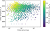 |
Fig. 1 Catalogue of exoplanets discovered to-date, showing the diversity of stellar temperatures and orbital periods. In colour: the planet equilibrium temperature (grey for planets where this is not given). The line of seven points at the bottom is the TRAPPIST-1 system. The catalogue is taken from the confirmed planets discovered by RV and transits from exoplanet.eu (updated 23/12/19). |
2 Data
2.1 Target characterisation
Our targets are taken from a number of Guest Observer programs focusing on ultracool stars and brown dwarfs and containing 1310 unique EPIC numbers. In several cases, however, two EPICs were found to refer to the same target. After resolving all duplicates and performing the target selection described below, we are left with 702 unique characterised ultracool dwarfs for the occurrence rate estimation. Some of the stars have observations spanning multiple campaigns; for such cases, we take the detection sensitivity of the light curve with the best detrended noise characteristics (see Sect. 3.1). We did not include targets from Campaign 1 due to the weaker photometric quality or Campaign 9 as it focused on microlensing.
We first characterise the target stars to find their radii and masses. We use these parameters to filter out our ultracool dwarf sample and remove any mis-classified stars. Distant red giants can masquerade as bright ultracool stars, as they have similar surface temperatures and colour indices (Mann et al. 2012; Dressing et al. 2017b). Including these in our sample would significantly affect our results: red giants tend to be brighter and have more precise photometry than ultracool stars, which would cause us to overestimate our sample detection sensitivity. We can distinguish between red giants and cool dwarfs with the parallaxes provided by Gaia.
We perform our own stellar characterisation, as the KIC and EPIC values have been found to underestimate radii for low-mass stars by up to 39% (Brown et al. 2011; Boyajian et al. 2012; Huber et al. 2016; Dressing et al. 2017b). Cross-referencing with Gaia DR21 (Marrese et al. 2019) and 2MASS (Skrutskie et al. 2006), we find full five-parameter astrometric solutions for 1143 individual EPIC identifiers, which we use to estimate distances to the stars. We then perform spectral energy distribution (SED) fitting on each target with the combined Gaia and 2MASS photometry using the Virtual Observatory Spectral Energy Distribution Analyser2 (VOSA; Bayo et al. 2008; Rodrigo et al. 2017). We use the Virtual Observatory catalogues to also add photometric magnitudes from other sources, for example including WISE (Wright et al. 2010), SDSS (Aguado et al. 2019), UKIDSS (Lawrence et al. 2007), and PAN-STARRS (Chambers et al. 2016) where available. We fit the SEDs with the BT-Settl, BT-COND, BT-DUSTY (Allard et al. 2012), and BT-Settl-CIFIST (Baraffe et al. 2015), selecting the highest-likelihood model with the VOSA tool. For each star, we thus obtain the stellar effective temperature, Teff ; and where the parallax is known, the luminosity,  .
.
We also cross-reference our target sample with the online census compiled by J. Gagné3. This list contains well-characterised ultracool dwarfs and brown dwarfs taken from various sources in the literature, and also includes spectral types. Our SED-derived spectral types agree with the values in the Gagné census to within two spectral subtypes for 97% of cases, and within one spectral subtype for 88% of cases. We also find that the difference in the stellar indices is symmetrically distributed, meaning that we are not biased to over- or underestimating the stellar temperatures compared to previously published values.
In selecting our targets, we first cut out all targets with SED-derived Teff > 3000 K and Rstar > 0.5 R⊙. The high radius cut allows us to keep faint stars with poor precision on their parallax measurements (see Fig. 2). We find a number of targets with very imprecise parallaxes; 213 EPIC numbers have a parallax-over-error of less than 10. For these targets, the stellar radii are very uncertain and biased to higher values.
A number of faint targets present in the J. Gagné list are also missing parallaxes or were not found in Gaia DR2. We cannot directly infer  for these stars, but the majority of targets with missing parallaxes have very faint magnitudes – clustered around a Gaia G-band magnitude of 20. For the 20 targets with Gaia data but missing astrometry, the mean and brightest G magnitudes are 20.1 and 16.7 respectively, while the mean and brightest 2MASS J-band magnitudes are 15.9 and12.4 respectively. For another 94 targets that could not be cross-matched to Gaia DR2, we find mean and brightest 2MASS J magnitudes of 16.0 and 11.1 respectively. All of these targets are characterised as ultracool or brown dwarfs in the J. Gagné census, and are unlikely to be mis-characterised red giants due to their low magnitude (see Mann et al. 2012). We therefore include them in our target list.
We also check the detrended noise of each target as a function of its Gaia G magnitude (see Sect. 3.1 for the detrending procedure). A number of targets have a noise level below what we would expect based on the magnitude, which could be due to the PSF of those targets being blended with a brighter star. We filter out 87 such targets.
It should be noted that TRAPPIST-1 is not part of our stellar sample. While it was included in a Guest Observer proposal for campaign 12 – before the discovery of its planets – the star itself would have fallen just outside one of the CCD frames in the initial observation field. Only after the discovery of the planets by Gillon et al. (2016) was the campaign 12 field modified to include TRAPPIST-1. The presence of TRAPPIST-1 in our sample would therefore be conditioned on it having an already discovered system. Without modelling for this selection bias, we cannot include TRAPPIST-1 in the sample.
To calculate transit depths, we must input values for stellar radii and masses. Targets with imprecise parallaxes have large uncertainties in stellar radii; in some cases, the means of the radii are inconsistent with ultracool dwarf isochrones and evolutionary tracks. We therefore use the following treatment: we use our SED-derived Teff to match toa spectral type, and take the corresponding stellar radius from the table compiled by E. Mamajek4 (Pecaut & Mamajek 2013). For targets with no parallaxes, we use the spectral type quoted in J. Gagné instead. In total, our filtered catalogue contains 702 unique targets, with 644 M Dwarfs, 46 L Dwarfs, and 3 T Dwarfs.
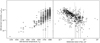 |
Fig. 2 Distribution of stellar parameters for our filtered targets. Left: SED-derived temperatures and luminosities. Right: SED-derived luminosity and the fractional noise in the fully detrended light curve of each target. Faint targets (with high noise in the light curve) have large uncertainties in their parallaxes and therefore their luminosities. |
2.2 Light curve photometry
For each target, we download the long-cadence (~30 min exposure) target pixel files (TPFs), and perform the photometry ourselves, rather than using the light curves processed by the Kepler/K2 SOC. For dim targets, we find that using our custom pipeline improves our final photometricprecision over the PDC light curves, and this also allows us to better control our systematic noise5.
Some of the targets are referenced by multiple EPIC numbers, with separate TPFs for each within the same campaign (usually on the order of 10 arcseconds apart). When this occurs, we use the Gaia proper motions to estimate the position of the target during the observation, and take the EPIC with the closest listed coordinates.
Due to its failed reaction wheels, the pointing angle of K2 is constantly drifting and being corrected by thruster firings (Howell et al. 2014), meaning that the targets move across their TPFs over a timescale of ~ 6 h. To perform the photometry, we use circular top-hat apertures following each target, with a two-pixel radius. To begin with, we search within 1.5 pixels of the predicted position to lock on to the target, using the WCS header in each TPF to transform astrometric into pixel coordinates. We repeat this procedure on 100 randomly selected frames to find the median offset from the expected position. Each TPF provides estimated pointing offset coordinates for each frame in XPOS_CORR and YPOS_CORR in units of pixels. To ensure the aperture follows the target, we offset it by XPOS_CORR and YPOS_CORR in each frame.
Finally, we remove points that are next to thruster-firing events, as well as other points flagged in the TPF QUALITY column (Jenkins et al. 2010). We find that our photometric procedure already removes a significant portion of the systematic noise present in the PDC light curves.
3 Transit-search pipeline
To estimate occurrence rates, we need to calculate the completeness of our search; meaning the probability of finding a planet for a particular target, if it were there. We must first create an automatic pipeline which encompasses all the data processing, including the removal of noise and the subsequent transit search. As our target stars are faint, which limits our photometric precision, we must make every effort to maximise the quality of our data and remove as much noise as possible. The entire pipeline must be computationally efficient, as we will repeat it thousands of times per target (see Sect. 4).
3.1 Detrending
The light curves produced by K2 photometry are well known to suffer from correlated systematic noise. This is caused by the unstable pointing vector of the spacecraft, which drifts on six-hour timescales and needs to be re-positioned with thruster firings to keep it on target. As each pixel has an (unknown) pixel-response-function (PRF), this drift introduces noise into our photometric light curve, which can be larger than the transit signals we are looking for. As a consequence, the pointing-drift noise is strongly correlated with the x and y positions of the star on the TPF. Additionally, many stars exhibit stellar variability, producing either a long-term and smooth variation in flux, or shorter timescale variations which are generally quasi-periodic.
Most transit-search algorithms require a flattened light curve, and short-timescale systematic noise can mimic transit signals. Removing both sources of systematic noise while preserving potential transit dips is a crucial step in our data analysis pipeline.
To that end, we use Gaussian process (GP) regression to fit for both sources of noise simultaneously, allowing us to remove them (referred to as detrending). Gaussian processes are a popular way to remove systematic signals from K2 data (see Aigrain et al. 2016, on which our procedure is based). We only present a brief outline here.
Our GP model uses three predictors: the time, t, as well as the x and y positions of the star on the TPF. The basic version of our model uses decaying squared-exponential kernels in each of those parameters:
 (1)
(1)
where i, j index two different points in thelight curve and δij is the Kronecker delta function, and where:

On a subset of light curves, we also tested the performance of the Matérn 5/2 kernel, which places fewer restrictions on the smoothness of the fit. The average difference in performance was not significant, though in the future it may be worth selecting the kernel on a case-by-case basis, depending on which shows better detrending performance for a given light curve.
Before conducting the full detrending procedure, we perform a short run and calculate a Lomb-Scargle periodogram of the time-correlated component of our light curve. If a periodicity is detected above a certain threshold, we instead use a quasi-periodic kernel for the time parameter:
 (4)
(4)
Our pipeline is re-purposed from the one used in Luger et al. (2017) and Grimm et al. (2018), with modifications for the increased speed required here. We perform four consecutive hyperparameter fits in a process similar to sigma clipping in order to flag outliers that will be ignored in subsequent GP fits. Masking the outliers is only relevant during the detrending stage; they are not removed for the transit search. During the hyperparameter-fitting procedure, we use a subset of the flux measurements to calculate the likelihood at each iteration. We only use the full light curve for the predicting the noise components,that is, during the outlier flagging and during the final detrending. We show an example of the detrending results in Fig. 3.
Having fit the systematic noise, we then subtract it from the light curve, in order to produce the flattened light curves on which we perform the transit search. For many targets, we also notice a ramp-like feature in the beginning of the light curve. Where this feature is detected, we fit it simultaneously with the GP hyperparameters using an exponential function and subtract it as well. The Gaussian process regression is implemented using the george package in python (Ambikasaran et al. 2015).
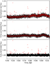 |
Fig. 3 Example of the detrending procedure for target EPIC 212035051 in campaign 5. The improvement in the flux standard deviation is from 0.008 for the raw light curve to 0.004 for the detrended light curve. Top: raw flux. Middle: time-correlated component, mostly quasiperiodic stellar variability, with pointing drift noise removed. Bottom: detrended light curve on which we perform the transit search. Red points are outliers at more than 3 standard deviations from the trend. They are masked out during the detrending; i.e. we do not use them to predict the noise trend. |
3.2 Transit search
We then perform a standard transit-search; see e.g. Dressing & Charbonneau (2015), Vanderburg et al. (2016), and Mayo et al. (2018) for similar procedures. We first calculate a series of box-fitting-least-squares (BLS) spectra to find periodic dips in our data (Kovács et al. 2002). We modify the BLS algorithm to only search for dip durations shorter than the maximum transit duration at a particular period with a 3× tolerance factor. We also limit the search resolution to the minimum required for a particular period, with 2× tolerance. These steps greatly speed up the BLS procedure.
At each iteration, we note the peak in the BLS spectrum, corresponding to the “strongest” periodic dips (see Kovács et al. 2002). We then remove the points within two durations of each dip, before rerunning the BLS algorithm to search for more signals. We test each peak by removing the two points with the lowest flux; if this changes the average depth of the peak by more than 50% we flag the peak as invalid. Peaks with negative depths are also flagged as invalid. This is repeated until ten valid peaks are found.
We then perform a physical transit model fit on each valid BLS peak. The model used is based on Mandel & Agol (2002) and implemented in the batman package (Kreidberg 2015). From this we obtain joint distributions for the planet radius, period, first-transit time t0 and impact parameter. We assume zero eccentricity, as the planets we search for are all in close-in orbits.
For each fit, we calculate a signal-to-noise ratio (S/N), defined as
 (5)
(5)
where d is the transit depth, Np is the number of points in transit, and σ is estimated in the fitted GP model of the light curve (see Eq. (1)). Here, σ is therefore the sigma-clipped standard deviation of the detrended light curve. Valid BLS peaks that produce an S/N greater than 7 are passed to visual inspection. From visual inspection, we can discard peaks that are clearly noise or anomalies, and keep peaks that could potentially be transits. Obvious and common systematic noise includes points near thruster firings, displaying a clear ramp going into the thruster firing event. This also produces a very asymmetric dip. Occasionally, we also noticed temporary bouts of heavily increased white noise, where a few points below the flux median could produce a high-S/N dip.
3.3 Transit-search results
We test our detrending and transit-search pipeline on TRAPPIST-1, finding six of the seven planets. The last planet, TRAPPIST-1h, only has four transits in the K2 data, with one occurring during a flare, and one overlapping with a transit from planet b (Luger et al. 2017). As the smallest planet in the system, its discovery was very near K2’s detection limit. Without using prior knowledge to search for it – as was done when possible periods and ephemerides were predicted from Laplace resonances in Luger et al. (2017) – it is unsurprising that it cannot be found.
Performing the search across our entire sample of targets, our pipeline identifies 116 potential transit signals. We examine these visually, and we also perform a search for possible aliases by focusing on alternate peaks in the BLS spectrum. The majority of signals near our S/N limit are caused by residual noise in the light curve. This is mostly caused by stellar variability below our detection limit, limited sections of the light curve with increased noise, or instances where the star drifts off the TPF aperture. Some light curves also have leftover red noise at timescales below what we detrended.
Out of the filtered signals, we find five credible transit-like signals. Three of them are eclipsing binaries which have been previously identified in the literature; their EPIC numbers are 211079188 (Kruse et al. 2019), 212002525 (Gillen et al. 2017), and 211075914 (David et al. 2016). We find one clear planetary signal in EPIC 210490365, which corresponds to K2-25b. Our retrieval produces a radius of 1.7 ± 0.2 R⊕. Mann et al. (2016) identified this as a Neptune-sized planet, with a radius of  and a period of 3.43 days. Mann et al. (2016) use the star’s membership in the Hyades cluster to estimate its distance, which they use to calculate the luminosity. For the radius and mass estimate, however, these latter authors use the relations derived in Mann et al. (2015); the estimates are significantly larger than the model values we use based on an M5.5V dwarf (see Sect. 2). For the occurrence rate calculation, we adopt their published values and uncertainties for the radius and period, which include their stellar radius uncertainty.
4 Detection sensitivities
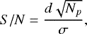
In order to estimate the occurrence rates of planets from our data, we need to know our detection sensitivity as a function of the planet parameters (i.e. the chance of finding a planet given that it transits). Each light curve has a different noise profile, and the most accurate way to find our detection sensitivity is to directly test our transit-search pipeline on the real light curves themselves. We perform injection-recovery modelling using batman (Kreidberg 2015), injecting 1000 synthetic transit signals per light curve and using random planetary and/or orbital parameters. Each injected synthetic signal has planetary radius, orbital period, inclination, and eccentricity (Rp, P, i, e) taken from the following distributions:
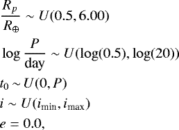
where imax and imin are calculated for each star as the maximum and minimum inclination for a transit, and where ~ U(a, b) signifies that a random variable is “drawn from a uniform distribution between a and b”. We fix the eccentricity at 0.0, as we do not know the underlying eccentricity distribution. This assumption has a small effect; close-in planets around ultracool dwarfs are subject to strong orbital circularisation (see e.g. Luger et al. 2017). The distribution of injected radii and periods is taken to match the distribution of the bins we use to parametrise the detection efficiency and occurrence rate (see Sects. 5 and 6.1).
We then run our entire transit-search pipeline on each modified light curve, and attempt to retrieve the transit parameters. This includes the detrending stage, as it can in principle remove or smear out transit signals. In order to count as a detection, we have the following tolerances: the detected period must match to within 1%, the time of first transit must match to within half a transit duration, and the duration must match to within 50% of the injected duration. Period aliases of the injected signal are treated as detections (though this naturally reduces their calculated S/N, which may lead to them being rejected). We look for alias periods at factors of  , and 3 of the injected period, with the same tolerance criteria as normal signals. We find an average of around three alias detections per 1000 injections.
We split the Rp and log P space into a set of NB bins,  , and count the fraction of injections that were recovered in each bin. There is a trade-off between the size and number of bins we use, and the number of injections we need to make per light curve. With smaller bins, the distribution of injected radii and periods within each bin is less important, and we better approximate the true smooth nature of the planetary occurrence rate distribution.However, to maintain the same level of per-bin sampling, decreasing the bin size requires an increase in the number of injected signals per light curve by the same factor.
We do not include visual identification as a step in the injection-recovery modelling because of the sheer number of light curves produced. This is a potential source of bias, and is equivalent to assuming that we would not incorrectly identify a real transit as noise if it got past all the stages of our transit search. This is also why we had to make our pipeline strongly automated and capable of discarding as much noise as possible on its own: to reduce our reliance on visual identification.
As a result, we must be careful in Sect. 3 in deciding which features to consider as noise. The rejected signals must have a feature that clearly sets them apart from a physical transit. If we remove transit-like signals that could be produced by our physical model, we may then also remove actual transit signals. Moreover, we would have to apply the same selection criterion in removing injected signals, and as we do not visually inspect the injected signals, this would bias our results.
The fraction of injected planet signals that are detected in a particular light curve, as a function of planet period and radius, is taken as the detection sensitivity in that bin, ηdet. A plot of our sample-wide detection sensitivity is shown in Fig. 4a, integrated over the entire sample of targets.
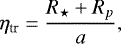
For a given planet injection, we can also calculate the geometric transit probability, given by
 (6)
(6)
where a is the orbital semi-major axis, and R⋆ is the radius of the star.
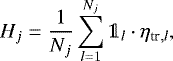
Finally, for a particular star and within a particular bin, Bj, we approximate the average completeness, Hj. We take the completeness as the number of detected injections weighted by the transit probability of each injection, and divide by the total number of injections falling inside the bin, Nj :
 (7)
(7)
where  is the geometric transit probability of the lth injection, and where
 (8)
(8)
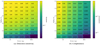 |
Fig. 4 Left: detection sensitivity, showing the chance of finding a planet in the data given that it is transiting, shown as a function of planet radius and orbital period. Right: completeness, showing the chance of finding a planet with a random orbital alignment. In both cases, we integrate over the entire sample of 702 stars, thus showing the mean of the sensitivity or completeness across our entire sample. For example, if TRAPPIST-1b (R =1.086, P =1.51d, Gillon et al. 2017) were orbiting a random star in our sample, we would have a 0.77% chance of finding it given a random inclination, or a 12% chance of detecting it if it was transiting. |
5 Modelling the occurrence rate
We treat planet detections as being drawn from an inhomogeneous Poisson point process. In other words, for the ith star, the detection of a planet with radius and orbital period (Rp, P) is an event that occurs with a rate λi which depends on (Rp, log P)6. We henceforth denote our planet parameters as x = (Rp, log P).
The ratedensity of planet detections, λi(x), is the resultof several probabilistic steps. Firstly, there is a true planetary occurrence rate, η, which determines the number of planets per star in our sample, including non-detections. This is the unknown quantity we seek to find, and we take it to be the same for all the stars in our sample. Of the planets that may orbit the stars in our sample, only a fraction will have orbits aligned so that they transit from our point of view. We refer to this fraction as the geometric transit probability, ηtr (see Eq. (6)). Finally, only a fraction of the transiting planets will be detected by our pipeline. Depending on the size of the signal and the number of transits, there is a chance our pipeline cannot distinguish it from noise. Included in this is the chance that transits fall within gaps in the data. We calculate this detection sensitivity, ηdet, through injection-recovery modelling for each star (see Sect. 4). We combine the detection sensitivity and transit probability into the completeness, H = ηtrηdet.
The total rate of planet detections is then given as the product of these probabilities λi = ηHi for each star indexed by i, where each of those quantities depends on (Rp, log P). Once we can calculate  and
and  , and thus Hi, we can use our data (detections and non-detections) to infer the occurrence rate, η.
To make the problem computationally tractable, we split our parameter space, x = (Rp, log P), into a set of NB bins:  . Treating the occurrence rate as constant within a bin, the parameters we seek to infer are the occurrence rates within the individual bins:
  . We then also treat the completeness as constant within each bin, and equal to the average completeness we calculate in Eq. (7).
In the following sections, we present the likelihood functions that we use to infer the occurrence rate parameters, η. We first do this for the case where the parameters of detected planets are precisely known (without uncertainties), and then extend that to working with uncertain planet parameters.
5.1 Precisely-known planet parameters
The likelihood of a Poisson point process is easily defined when we know the precise values of events drawn from it, where events correspond to planet detections. For the ith star, we count the number of real planet detections in bin Bj and denote it dij. For an inhomogeneous Poisson process on this parameter space (see e.g. Daley & Vere-Jones 2007), with a rate function λ(x), the likelihood function for set of detections around the ith star is:
 (9)
(9)
where the measure Λ(Bj) is the integrated rate in bin Bj, defined as:
 (10)
(10)
Within our framework, as the occurrence rate and completeness are taken to be constant within each bin, we can simplify Λ(Bj) to
 (11)
(11)
where |Bj| is the volume of bin Bj, and Hij is the completeness in bin Bj for the ith star.
Assuming that the data for each star is independent, our total likelihood, for all N⋆ stars in our sample, is then:

We only need to know the likelihood up to a multiplying constant, so we can remove any factors that do not depend on η, and we can further simplify the likelihood to obtain
![\begin{align*} L(\bm{\eta}) & \propto \prod_{j=1}^{N_B} \eta_j^{\sum_{i=1}^{N_{\star}} d_{ij}} \exp \left( - \eta_j |B_j| \sum_{i=1}^{N_{\star}} {H}_{ij} \right) \\ & = \prod_{j=1}^{N_B} \eta_j^{D_j} \exp \left( - \eta_j N_{\star} \bar{{H}} _j |B_j| \right) \\ & = \left[ \prod_{j=1}^{N_B} \eta_j^{D_j} \right] \exp \left( - \sum_{j=1}^{N_B} \eta_j N_{\star} \bar{{H}} _j |B_j| \right),\end{align*}](/articles/aa/full_html/2020/09/aa37732-20/aa37732-20-eq24.png)
where  is the total number of real planet detections in bin Bj across all the stars in our sample, and
  is the mean completeness in bin Bj across our whole sample. Here,
  is the quantity plotted in Fig. 4b, and can be written:
 (18)
(18)
The expectation of the total number of planet detections is equal to the term in the exponential of Eq. (17) (see Youdin 2011):
 (19)
(19)
We note that Nexp will also appear in the likelihood we derive for uncertain planet parameters.
5.2 Planet parameters with uncertainties
The likelihood in Eq. (17) assumes that the planet radii and periods are known precisely, without uncertainties. This is not the case for a real catalogue of detections. To correctly treat uncertain planet parameters in our Bayesian formulation, we must use a hierarchical/multi-level Bayesian model (HBM). In the first application of an HBM in modelling planetary occurrence rates, Foreman-Mackey et al. (2014) show that an HBM recovers the underlying parameters of simulated data with a higher accuracy than traditional methods. We point the reader to Foreman-Mackey et al. (2014) for an explanation and justification of the principles of using a hierarchical framework to model planetary occurrence rates, and its advantages over traditional methods (see also e.g. Hogg et al. 2010, for a more general introduction of HBMs in astrophysics).
In this section, we formulate our HBM, and show a convenient way to write the likelihood function in terms of only the parameters we are interested in (the occurrence rates, η). We can therefore sample the parameters of our HBM as if it were a two-level model. Starting with the general likelihood equation for a Poisson point process, for the ith star, we can rewrite Eq. (9) as:
![\begin{align*} L_i & = \left[ \prod_{j=1}^{N_B} \frac{(\Lambda_i (B_j))^{d_{ij}}}{d_{ij}!} \right] \exp \left(-\sum_{j=1}^{N_B} \Lambda_i (B_j) \right) \\ & = \left[ \prod_{j=1}^{N_B} \frac{(\Lambda_i (B_j))^{d_{ij}}}{d_{ij}!} \right] \exp \left(- N_{\text{exp,i}} \right),\end{align*}](/articles/aa/full_html/2020/09/aa37732-20/aa37732-20-eq30.png)
where we have the expectation of the total number of planet detections for the ith star,  . Assuming that the bins
  fully tile our parameter space, the value of Nexp,i is independent from how we choose the bin boundaries.
Equation (21) works for an arbitrary set of bins as long as they are disjoint and cover the entire parameter space. Taking this to an extreme, we can choose the bin boundaries such that for each detected planet, there exists a bin that contains the parameters of only that planet; thus no bin holds two planets. We can also arbitrarily decrease the size of the bins that contain a planet. In the limit of infinitesimally small bins, we can write:

where  is a point in the bin B′, |B′ | is the volume of the bin, and we denote the new set of bins with a prime to differentiate for later. Since only the bins containing planets will appear in the product of Eq. (21), we can write the equation as:
![\begin{equation*} L_i = \left\{ \begin{array}{ll}\displaystyle \left[ \prod_{l=1}^{d_i} \lambda_i (\boldsymbol{x}_{il}) |B_{il}'| \right] \exp \left(- N_{\text{exp,i}} \right), & \text{for } d_i \geq 1 \\[5pt] \displaystyle \exp \left(- N_{\text{exp,i}} \right), & \text{otherwise,}\end{array} \right.\end{equation*}](/articles/aa/full_html/2020/09/aa37732-20/aa37732-20-eq35.png) (24)
(24)
where di is the total number of planet detections for star i, and we use l to index over the planets detected around star i; thus xil are the parameters of the lth planet of star i.
The above still assumes that we have precise knowledge of the true planet parameters, xil. However, in reality, the true parameters xil of a detected planet are not known. Instead, our observations produce a set of measured values,  , drawn from some uncertainty distribution,
  , where αil parametrise the uncertainty distribution. For a Gaussian uncertainty distribution, αil can be the variance, that is, the error-bars squared, with xil as the mean. αil itself depends on the light curve quality; the stellar parameters and their uncertainties, and so on.
The likelihood we are now interested in is the likelihood of measuring particular values for a set of detected planets; it includes two probabilities. Firstly, the probability of a set of planets being detected, given some model parameters for the detection rate, η, and defined in terms of the true parameters of the planets, xil; and secondly, the probability of measuring the values  for those parameters. We denote this new likelihood with a tilde,
  ; if the ith star has at least one planet detection, the likelihood is:
![\begin{align} & \tilde{L}_i = p \left(\{\boldsymbol{\tilde{x}}_{il}\}_{l=1}^{d_i} \;\middle|\; \boldsymbol{\eta}, \{\boldsymbol{\alpha}_{il}\}_{l=1}^{d_i} \right) \\ & = \int p \left(\{\boldsymbol{\tilde{x}}_{il}\}_{l=1}^{d_i} \;\middle|\; \{\boldsymbol{x}_{il}\}_{l=1}^{d_i}, \{\boldsymbol{\alpha}_{il}\}_{l=1}^{d_i} \right) p \left(\{\boldsymbol{x}_{il}\}_{l=1}^{d_i} \;\middle|\; \boldsymbol{\eta} \right) \textstyle\prod _{l=1}^{d_i} \textrm{d}\boldsymbol{x}_{il} \\ & = \int\! \left[ \prod_{l=1}^{d_i} p \left(\boldsymbol{\tilde{x}}_{il} \;\middle|\; \boldsymbol{x}_{il}, \boldsymbol{\alpha}_{il} \right)\right] \left[ \prod_{l=1}^{d_i} \lambda_i (\boldsymbol{x}_{il}) |B_{il}'| \right] \exp \left(- N_{\text{exp,i}} \right) \textstyle\prod _{l=1}^{d_i} \textrm{d}\boldsymbol{x}_{il}\\ & = \left[ \prod_{l=1}^{d_i} |B_{il}'| \int \lambda_i (\boldsymbol{x}_{il}) p \left(\boldsymbol{\tilde{x}}_{il} \;\middle|\; \boldsymbol{x}_{il}, \boldsymbol{\alpha}_{il} \right) \textrm{d}\boldsymbol{x}_{il} \right] \exp \left(- N_{\text{exp,i}} \right).\end{align}](/articles/aa/full_html/2020/09/aa37732-20/aa37732-20-eq40.png)
Equation (27) is obtained by substituting the previously derived form of the likelihood for a Poisson point process, Eq. (24) into  , and using the fact that the measured values of the planets are conditionally independent given α, which in principle includes the stellar parameters and their uncertainties7. It should also be noted that this assumes that the detection efficiencies for multiple planets orbiting the same star are independent of each other. If the ith star has no planet detections, there is no parameter uncertainty, and the likelihood is:
 (29)
(29)
We now consider the likelihood over the entire set of stars in our sample,  . We can write it as a product of the individual likelihoods of the stars because we assume that the planet detections we make for individual stars are independent of each other. Most stars will not have any detected planets; the likelihood functions of these stars will come from Eq. (29). The product in Eq. (28) will only appear where there is a detected planet. Additionally, we can ignore any multiplicative constants in our likelihood; so we drop
  . The total likelihood is then:
![\begin{align*} \tilde{L} & \propto \left[ \prod_{l=1}^{D} \int \!\lambda_{i(l)} (\boldsymbol{x}_{i(l)l}) p \left(\boldsymbol{\tilde{x}}_{i(l)l} \;\middle|\; \boldsymbol{x}_{i(l)l}, \boldsymbol{\alpha}_{i(l)l} \right) \textrm{d}\boldsymbol{x}_{i(l)l} \right] \prod_{i=1}^{N_{\star}} \exp \left(- N_{\text{exp,i}} \right) \\ & = \left[ \prod_{l=1}^{D} \int \lambda_{i(l)} (\boldsymbol{x}_{i(l)l}) p \left(\boldsymbol{\tilde{x}}_{i(l)l} \;\middle|\; \boldsymbol{x}_{i(l)l}, \boldsymbol{\alpha}_{i(l)l} \right) \textrm{d}\boldsymbol{x}_{i(l)l} \right] \exp \left(- N_{\text{exp}} \right),\end{align*}](/articles/aa/full_html/2020/09/aa37732-20/aa37732-20-eq45.png)
where we are now using l to index over all D detected planets in our entire stellar sample, and where i(l) denotes the index of the star that hosts the lth planet. The quantity  is the expectation of the total number of detected planets in our entire stellar sample (see Sect. 5.1).
We now reintroduce our previous parametrisation for λi (xil): we split the parameter space x = (Rp, log P) into bins, within which the completeness, occurrence rate, and therefore λi, are constant (see Sect. 5.1). This allows us to split the integrals in Eq. (31) into sums of integrals over each bin. The set of bins we use here,  , is not related to the set of bins we used to obtain Eq. (23). The likelihood becomes:
![\begin{align*} \tilde{L} & \propto \left[ \prod_{l=1}^{D}\sum_{j=1}^{N_B} \lambda_{i(l)j} \int_{B_j} p \left(\boldsymbol{\tilde{x}}_{i(l)l} \;\middle|\; \boldsymbol{x}_{i(l)l}, \boldsymbol{\alpha}_{i(l)l} \right) \textrm{d}\boldsymbol{x}_{i(l)l} \right] \exp \left(- N_{\text{exp}} \right) \\ & = \left[ \prod_{l=1}^{D} \sum_{j=1}^{N_B} \lambda_{i(l)j} F_{i(l)jl} \right] \exp \left(- N_{\text{exp}} \right) \\ & = \left[ \prod_{l=1}^{D} \sum_{j=1}^{N_B} {H}_{i(l)j} \eta_{j} F_{i(l)jl} \right] \exp \left(- N_{\text{exp}} \right),\end{align*}](/articles/aa/full_html/2020/09/aa37732-20/aa37732-20-eq48.png)
where λij = Hijηj is the (constant) detection rate within bin Bj, for the ith star, and where we define:
 (35)
(35)
Our final likelihood in Eq. (34) may appear more complicated than Eq. (17); however, in practice it is simple to calculate. We need to calculate the terms Fijl only once; it does not need to be updated as we infer the occurrence rate. We can calculate Fijl with a Monte Carlo sampling scheme for example. The same is true for the completeness Hij, as before (see Sects. 4 and 5.1). The quantity Nexp is the same as in Sect. 5.1, and can be calculated with Eq. (19); it is independentof the planet detections themselves. It is also not difficult to calculate the Jacobian of  with respect to η, which allows us to later use gradient-based sampling methods (see Sect. 5.3).
The method presented here is general, and can be applied to any occurrence rate study where the completeness and occurrence rate distribution are parametrised with a piecewise-constant step-function, which is very popular in the literature (see e.g. Howard et al. 2012; Dong & Zhu 2013; Swift et al. 2013; Dressing & Charbonneau 2015; Mulders et al. 2015a; He et al. 2017). The alternative would have been to infer the full joint-posterior distribution of the HBM, including a set of parameters x = (Rp, log P) for each detected planet. This would add two model parameters per detected planet, and more if we wanted to find the relation between planetary occurrence rates and other parameters, such as stellar metallicity or stellar mass. With the single planet detection in our study, the difference is not large. However, in general, studies such as Dressing & Charbonneau (2015) can include hundreds of planet candidates, which rapidly inflates the number of parameters we need to infer. Directly marginalising over the planet parameters can therefore lead to a significant increase in computational speed with such large planet samples, which our method avoids.
5.3 Posterior distribution of η
We infer the occurrence rates within a Bayesian framework, and our posterior distribution on η is given by:
 (36)
(36)
where we use the Jeffreys prior for the rate parameters of a Poisson process:
 (37)
(37)
We draw samples from the posterior using Markov chain Monte Carlo sampling methods. When dealing with a smaller number of model parameters (in Sect. 6.2), we use the affine-invariant sampler implemented in emcee (see Goodman & Weare 2010; Foreman-Mackey et al. 2013); however, for larger numbers of parameters we find that this latter does not perform as well as gradient-based samplers. As we have closed-form equations for our likelihood and our prior, we also directly calculate the gradient of p(η|data) with respect to η. This allows us to use Hamiltonian Monte Carlo samplers, such as the No-U-Turn Sampler implemented in PyMC3, for much faster convergence (Hoffman & Gelman 2014; Salvatier et al. 2016).
6 Results
6.1 Occurrence rates
We consider radii between 1 R⊕ and 6 R⊕ split into bins with an interval of 0.5 R⊕; and periods between 0.5 and 20 days split into regular intervals in log-period. Given only one detected planet in the sample, our constraints on the occurrence rate act mainly as upper limits. When referring to the upper limit on the occurrence rate, we henceforth refer to the 95th percentile in the posterior distributions for η; i.e. the upper bound on the 95% credible interval. As shown in red in Fig. 5, the occurrence rate upper limits follow a roughly inverted pattern from the completeness in Fig. 4b. The upper-left numbers in Fig. 5 show the expected number of planets we would detect if the occurrence rate had been equal to 1 within the bin. At larger radii and lower periods, where we have a better completeness, our constraints are stronger and lower, down to a few percent per bin. At radii below 1.5 R⊕ on the other hand, the occurrence rate cannot be constrained to below 1.0 for longer orbital periods because of the low completeness of our sample.
For super-Earths (1−2 R⊕), we find the occurrence rate to be in 95% credible intervals below 0.24, 0.41, 0.70, and 1.29, for period ranges of 0.5−0.9, 0.9−1.6, 1.6−2.8, and 2.8−5.0 days, respectively. Our constraint on the mini-Neptune (2−4 R⊕) population is stronger. Within the same period ranges, the 95% credible intervals for mini-Neptunes are below 0.12, 0.17, 0.28, and 0.53. In the 2.8−5.0 day bin, where we detect the sub-Neptune K2-25b, we also find an occurrence rate of  for mini-Neptunes. For planets above the size of Neptune (4−6 R⊕, referred to as gas giants from here), we find that there are fewer than 0.08, 0.12, 0.18, and 0.31 per star within those period ranges. The results are summarised in Table 1. We note that the 95% upper limit integrated across multiple bins is not equal to the sum of the 95% upper limits within each bin, as the upper limit depends on the distribution variance, which is not additive.
Occurrence rates for different planet classes: upper bounds on the 95% credible interval preceded by < where no detections are found, and median and 84% credible intervals as uncertainties for the bin containing K2-25b.
6.2 Occurrence rates integrated over period
To estimate the total occurrence rate within a period range such as 1− 0 days, we must sum the rate estimates over that range at a sample level. If we do this, however, the result will be dominated by the most poorly constrained bins, namely the bins at the upper end of the period range, where the completeness is lowest.
We can instead make the assumption that the occurrence rate is uniform in the log-period, within 1 − 20 days. This is consistent with previous results for earlier stellar classes (see e.g. Mulders et al. 2015a; Mulders 2018), and with the periods of the TRAPPIST-1 system. We re-run our analysis under this constraint, and integrate the occurrence rates within 1 − 20 days for each radius bin. The results are shown in Fig. 6. This is equivalent to calculating the occurrence rates with one large bin covering our entire period range.
The distributions on the resulting occurrence rates for super-Earths (1− 2 R⊕), mini-Neptunes (2− 4 R⊕), and ice/gas giants (4−6 R⊕) are summarised in Table 2. For super-Earths and ice/gas giants, where we have no detections, we find 95% upper limits of 1.14 and 0.29 planets per star. For mini-Neptunes with one detection, we find an occurrence rate of  planets per star, with a 95% upper limit of 0.54.
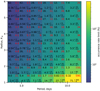 |
Fig. 5 Inferred occurrence rate as a percentage of our sample as a function of (Rp, log P). Within each bin, the numbers refer to the following quantities: top right: upper bound in 95% credible interval, i.e. the 95th percentile; top left: expected number of detections given an occurrence rate η = 1 within the bin, equal to |

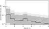 |
Fig. 6 Occurrence rate in our sample as a function of planet size. It is integrated over orbital periods of 1.0–20 days, assuming a uniform occurrence rate in log P within that range. The grey shaded regions show 84 and 95% credible intervals. |
Summary for the inferred distributions on the occurrence rates of super-Earths, mini-Neptunes, and ice/gas giants.
6.3 TRAPPIST-1-like systems
We do not find any planetary systems like TRAPPIST-1 in our sample. We can take our completeness for TRAPPIST-1-like systemsto be the probability of finding at least one of the planets if all seven were orbiting a star in our sample. With low mutual inclination, the completeness will depend on our ability to detect the most detectable planet in the system, TRAPPIST-1b. If we assume an occurrence rate for TRAPPIST-1-like systems within our sample, we can then calculate the probability of not finding any in our data (or conversely the probability of finding at least one). In the case where every ultracool dwarf in our sample held a system such as TRAPPIST-1, we would have a 4.2% chance of finding none (or a 95.8% chance of finding at least one). For a 20 and 5% system occurrence rate, the probability of finding at least one would be 46 and 14%, respectively.
7 Discussion
We find that gas giant planets are uncommon around ultracool stars, with fewer than 0.28 per star. We also improve upon the Demory et al. (2016) and He et al. (2017) constraints of mini-Neptune and super-Earth populations.Our results on the 95% upper limits are also in agreement with those of Sagear et al. (2020) across all planet classes.
The rarity of gas giants around low-mass stars has already been discussed in the literature (see e.g. Santos et al. 2004; Johnson et al. 2010; Gaidos et al. 2013; Obermeier et al. 2016; Mulders 2018). Short-period sub-Neptunes, however, have been found to become more common as stellar mass decreases (see e.g. Howard et al. 2012; Dressing & Charbonneau 2015; Mulders et al. 2015a,b; Muirhead et al. 2015). Collating the results of several studies in a review, Mulders (2018) showed that sub-Neptunes become approximately three times more common around M dwarfs relative to FGK stars8. The increased prevalence of small planets around low-mass stars is also predicted by formation synthesis models (e.g. Alibert & Benz 2017; Liu et al. 2019). However, Alibert & Benz (2017) find that larger planets such as mini-Neptunes are not reproduced by formation models for ultracool dwarfs. Whether the trend of increasing small planet occurrence rates continues into the late-M and brown dwarfs has not yet been observationally determined.
As an illustration of this trend, Fressin et al. (2013) found 0.066 ± 0.004 mini-Neptunes (2− 4 R⊕) and 0.096 ± 0.001 super-Earths (1.25−2 R⊕) per star at periods of 0.8−17 d for FGK stars in Kepler. In the sample of mostly mid- and early-M dwarfs observed by Kepler on the other hand, Dressing & Charbonneau (2015) found 0.29 planets with radii 2−4 R⊕ and periods 0.9 < P < 18.3 d, and 0.57 with radii 1−2 R⊕ (these are not upper limits, but averages). The other studies collated by Mulders (2018) show similar results; see e.g Youdin (2011), Howard et al. (2012), Dong & Zhu (2013), Petigura et al. (2013), Morton & Swift (2014), Mulders et al. (2015b), Silburt et al. (2015), Gaidos et al. (2016), and also Hsu et al. (2019, 2020).
Assuming uniform occurrence rates with log-period as in Mulders (2018) – without assuming uniformity in log-radius – we find that there are  mini-Neptunes per ultracool star (see Sect. 6.2). This is in line with the results for earlier M dwarfs, showing that the trend of high mini-Neptune occurrence rates is maintained for ultracool dwarfs. Such mini-Neptunes are larger than the range of radii reproduced by Alibert & Benz (2017), though this result relies on the detection of the mini-Neptune K2-25b, which appears to have an unusually large planet/star mass ratio9.
Extending the comparison to super-Earths (1−2 R⊕), we find that the integrated occurrence rate within 1−20d is within a 95% credible interval below 1.14, and within a 84% credible interval below 0.66. Using a well-characterised sample of M-dwarfs, Hardegree-Ullman et al. (2019) found that they host  planets per star at periods of 0.5−10 days and radii of 1.5−2.5 R⊕. To compare, our results within 1−10 orbital periods place a 95% upper limit of fewer than 0.36 planets of such size per star. The comparison depends on the assumed distribution of underlying planetary orbital periods: we assume that the occurrence rate density is uniform in log-period, while Hardegree-Ullman et al. (2019) set their distribution in period by sampling from the observed periods of their sample of 13 detected planets, 12 of which follow a roughly uniform distribution between 1 and 10 day periods. Muirhead et al. (2015) similarly find that
  of mid-M dwarfs host compact multi-planet systems with orbital periods of less than 10 days.
Overall, when compared with previous studies on mid- and early-M dwarfs, our results do not exclude a continuing trend of increasing occurrence rates for sub-Neptunes around lower mass stars. Further comparison would require more lower limits on the occurrence rate, which will be possible with more planetary detections.
With our completeness, if every ultracool dwarf hosted a TRAPPIST-1-like system, we would have a ~ 96% chance of finding at least one, based on the detectability of TRAPPIST-1b; however, this is strongly dependent on the 1.5 day period of the inner planet. Based on these facts, and that we do not detect any such systems, we can conclude that such short-periodsystems are not ubiquitous. The inner-planet periods may however be longer than those in TRAPPIST-1, allowing them to remain undetected in our sample. It is also possible that the formation of mini-Neptunes around ~ 20% of stars may inhibit the formation of long chains of rocky planets.
It has been suggested that inward migration of solids can explain the increased occurrence rate of short-period sub-Neptunes around low-mass stars (see e.g. Mulders et al. 2015a). Otherwise, we would expect the M dwarfs with lower disk masses to produce fewer and/or lower-mass planets. In future studies, it will be informative to test this hypothesis against spectral type and/or stellar mass, by directly constraining the distribution of occurrence rates as function of stellar mass. Instead of treating a sample of stars as a homogeneous set, an occurrence rate model could include a functional relation between the occurrence rate and stellar mass. With such data, we could directly test formation predictions that depend on stellar mass, such as pebble isolation enforcing a maximum super-Earth mass (Liu et al. 2019). However, this would make the computation more expensive, as simplifications such as Eqs. (14) into (17) would no longer be possible.
Given that TESS will not be sensitive to TRAPPIST-1-like systems around ultracool dwarfs (Sebastian et al., in prep), and K2 has finished its mission, our main chance of finding more rocky planets for atmospheric characterisation with JWST will come from ground-based surveys such as SPECULOOS and SAINT-EX. These surveys are aimed specifically at finding earth-sized planets around ultracool dwarfs, and they will provide much-needed completeness at low radii (Delrez et al. 2018). The downside will be that they have shorter observation timescales, and less completeness at longer orbital periods. Moreover, modelling their completeness is not trivial due to the daily gaps in the data and the likelihood of having to use single-transits as a detection criterion.
While most occurrence-rate studies tend to use data from a single survey, it is also possible to use the model in Sect. 5 on multiple surveys with different completeness functions. Combining the initial results of the SPECULOOS and SAINT-EX surveys with those of K2 will be crucial in further constraining the occurrence rate of Earth-sized planets. If such planetary systems prove to be uncommon, TRAPPIST-1 is likely to remain one of the unique few rocky planet systems that can be characterised by JWST.
Acknowledgements
The authors would like to thank Brett Morris for his helpful comments. M.S acknowledges support from the Swiss National Science Foundation (PP00P2-163967). B.-O.D. acknowledges support from the Swiss National Science Foundation in the form of a SNSF Professorship (PP00P2-163967). This work has been carried out within the framework of the NCCR PlanetS supported by the Swiss National Science Foundation. Calculationswere performed on UBELIX (http://www.id.unibe.ch/hpc), the HPC cluster at the University of Bern. This publication makes use of VOSA, developed under the Spanish Virtual Observatory project supported by the Spanish MINECO through grant AyA2017-84089. VOSA has been partially updated by using funding from the European Union’s Horizon 2020 Research and Innovation Programme, under Grant Agreement n° 776403 (EXOPLANETS-A). This paper includes data collected by the Kepler mission and obtained from the MAST data archive at the Space Telescope Science Institute (STScI). Funding for the Kepler mission is provided by the NASA Science Mission Directorate. STScI is operated by the Association of Universities for Research in Astronomy, Inc., under NASA contract NAS 5–26555. This study made use of data obtained within GO programs 2010, 2011, 3011, 3044, 3045, 3114, 4026, 4030, 4039, 4036, 4081, 5026, 5030, 5036, 5039, 5081, 6002, 6005, 6006, 7002, 7005, 7006, 8030, 8054, 10030, 10054, 11004, 11029, 11042, 12004, 12029, 12042, 13004, 13029, 13042, 14018, 14067, 15018, 15067, 16018, 16067, 17008, 17057, 18008, 18057 and 19008.
References
- Aguado, D. S., Ahumada, R., Almeida, A., et al. 2019, ApJS, 240, 23 [NASA ADS] [CrossRef] [Google Scholar]
- Aigrain, S., Parviainen, H., & Pope, B. J. S. 2016, MNRAS, 459, 2408 [NASA ADS] [Google Scholar]
- Alibert, Y., & Benz, W. 2017, A&A, 598, L5 [NASA ADS] [CrossRef] [EDP Sciences] [Google Scholar]
- Allard, F., Homeier, D., & Freytag, B. 2012, R. Soc. London Philos. Trans. Ser. A, 370, 2765 [Google Scholar]
- Ambikasaran, S., Foreman-Mackey, D., Greengard, L., Hogg, D. W., & O’Neil, M. 2015, IEEE Trans. Pattern Anal. Mach. Intell., 38, 252 [NASA ADS] [CrossRef] [Google Scholar]
- Ballard, S., & Johnson, J. A. 2016, ApJ, 816, 66 [NASA ADS] [CrossRef] [Google Scholar]
- Baraffe, I., Homeier, D., Allard, F., & Chabrier, G. 2015, A&A, 577, A42 [NASA ADS] [CrossRef] [EDP Sciences] [Google Scholar]
- Bayo, A., Rodrigo, C., Barrado Y Navascués, D., et al. 2008, A&A, 492, 277 [NASA ADS] [CrossRef] [EDP Sciences] [Google Scholar]
- Berta, Z. K., Irwin, J., & Charbonneau, D. 2013, ApJ, 775, 91 [NASA ADS] [CrossRef] [Google Scholar]
- Boyajian, T. S., von Braun, K., van Belle, G., et al. 2012, ApJ, 757, 112 [NASA ADS] [CrossRef] [Google Scholar]
- Brown, T. M., Latham, D. W., Everett, M. E., & Esquerdo, G. A. 2011, AJ, 142, 112 [NASA ADS] [CrossRef] [Google Scholar]
- Chambers, K. C., Magnier, E. A., Metcalfe, N., et al. 2016, ArXiv e-prints, [arXiv:1612.05560] [Google Scholar]
- Daley, D. J., & Vere-Jones, D. 2007, An Introduction to the Theory of Point Processes: Volume II: General Theory and Structure (New York: Springer Science & Business Media) [Google Scholar]
- David, T. J., Conroy, K. E., Hillenbrand, L. A., et al. 2016, AJ, 151, 112 [NASA ADS] [CrossRef] [Google Scholar]
- Delrez, L., Gillon, M., Queloz, D., et al. 2018, SPIE Conf. Ser., 10700, 107001I [Google Scholar]
- Demory, B.-O., Queloz, D., Alibert, Y., Gillen, E., & Gillon, M. 2016, ApJ, 825, L25 [NASA ADS] [CrossRef] [Google Scholar]
- Dong, S., & Zhu, Z. 2013, ApJ, 778, 53 [NASA ADS] [CrossRef] [Google Scholar]
- Dressing, C. D., & Charbonneau, D. 2013, ApJ, 767, 95 [NASA ADS] [CrossRef] [Google Scholar]
- Dressing, C. D., & Charbonneau, D. 2015, ApJ, 807, 45 [NASA ADS] [CrossRef] [Google Scholar]
- Dressing, C. D., Vanderburg, A., Schlieder, J. E., et al. 2017a, AJ, 154, 207 [NASA ADS] [CrossRef] [Google Scholar]
- Dressing, C. D., Newton, E. R., Schlieder, J. E., et al. 2017b, ApJ, 836, 167 [NASA ADS] [CrossRef] [Google Scholar]
- Fauchez, T. J., Villanueva, G. L., Schwieterman, E. W., et al. 2020, Nat. Astron., 4, 372 [CrossRef] [Google Scholar]
- Foreman-Mackey, D., Hogg, D. W., Lang, D., & Goodman, J. 2013, PASP, 125, 306 [CrossRef] [Google Scholar]
- Foreman-Mackey, D., Hogg, D. W., & Morton, T. D. 2014, ApJ, 795, 64 [NASA ADS] [CrossRef] [Google Scholar]
- Fressin, F., Torres, G., Charbonneau, D., et al. 2013, ApJ, 766, 81 [NASA ADS] [CrossRef] [Google Scholar]
- Gaidos, E., Fischer, D. A., Mann, A. W., & Howard, A. W. 2013, ApJ, 771, 18 [NASA ADS] [CrossRef] [Google Scholar]
- Gaidos, E., Mann, A. W., Kraus, A. L., & Ireland, M. 2016, MNRAS, 457, 2877 [NASA ADS] [CrossRef] [Google Scholar]
- Gillen, E., Hillenbrand, L. A., David, T. J., et al. 2017, ApJ, 849, 11 [NASA ADS] [CrossRef] [Google Scholar]
- Gillon, M., Jehin, E., Lederer, S. M., et al. 2016, Nature, 533, 221 [NASA ADS] [CrossRef] [PubMed] [Google Scholar]
- Gillon, M., Triaud, A. H. M. J., Demory, B.-O., et al. 2017, Nature, 542, 456 [NASA ADS] [CrossRef] [PubMed] [Google Scholar]
- Goodman, J., & Weare, J. 2010, Commun. Appl. Math. Comput. Sci., 5, 65 [Google Scholar]
- Grimm, S. L., Demory, B.-O., Gillon, M., et al. 2018, A&A, 613, A68 [NASA ADS] [CrossRef] [EDP Sciences] [Google Scholar]
- Hardegree-Ullman, K. K., Cushing, M. C., Muirhead, P. S., & Christiansen, J. L. 2019, AJ, 158, 75 [NASA ADS] [CrossRef] [Google Scholar]
- He, M. Y., Triaud, A. H. M. J., & Gillon, M. 2017, MNRAS, 464, 2687 [NASA ADS] [CrossRef] [Google Scholar]
- Hoffman, M. D., & Gelman, A. 2014, J. Mach. Learn. Res., 15, 1593 [Google Scholar]
- Hogg, D. W., Myers, A. D., & Bovy, J. 2010, ApJ, 725, 2166 [NASA ADS] [CrossRef] [Google Scholar]
- Howard, A. W., Marcy, G. W., Bryson, S. T., et al. 2012, ApJS, 201, 15 [NASA ADS] [CrossRef] [Google Scholar]
- Howell, S. B., Sobeck, C., Haas, M., et al. 2014, PASP, 126, 398 [NASA ADS] [CrossRef] [Google Scholar]
- Hsu, D. C., Ford, E. B., Ragozzine, D., & Ashby, K. 2019, AJ, 158, 109 [NASA ADS] [CrossRef] [Google Scholar]
- Hsu, D. C., Ford, E. B., & Terrien, R. 2020, MNRAS, 498, 2249 [CrossRef] [Google Scholar]
- Huber, D., Bryson, S. T., Haas, M. R., et al. 2016, ApJS, 224, 2 [NASA ADS] [CrossRef] [Google Scholar]
- Jenkins, J. M., Caldwell, D. A., Chandrasekaran, H., et al. 2010, ApJ, 713, L87 [NASA ADS] [CrossRef] [Google Scholar]
- Johnson, J. A., Aller, K. M., Howard, A. W., & Crepp, J. R. 2010, PASP, 122, 905 [NASA ADS] [CrossRef] [Google Scholar]
- Kopparapu, R. K. 2013, ApJ, 767, L8 [NASA ADS] [CrossRef] [Google Scholar]
- Kovács, G., Zucker, S., & Mazeh, T. 2002, A&A, 391, 369 [NASA ADS] [CrossRef] [EDP Sciences] [Google Scholar]
- Kreidberg, L. 2015, PASP, 127, 1161 [NASA ADS] [CrossRef] [Google Scholar]
- Kruse, E., Agol, E., Luger, R., & Foreman-Mackey, D. 2019, ApJS, 244, 11 [CrossRef] [Google Scholar]
- Lawrence, A., Warren, S. J., Almaini, O., et al. 2007, MNRAS, 379, 1599 [NASA ADS] [CrossRef] [MathSciNet] [Google Scholar]
- Liu, B., Lambrechts, M., Johansen, A., & Liu, F. 2019, A&A, 632, A7 [NASA ADS] [CrossRef] [EDP Sciences] [Google Scholar]
- Luger, R., Sestovic, M., Kruse, E., et al. 2017, Nat. Astron., 1, 0129 [Google Scholar]
- Lustig-Yaeger, J., Meadows, V. S., & Lincowski, A. P. 2019, AJ, 158, 27 [NASA ADS] [CrossRef] [Google Scholar]
- Mandel, K., & Agol, E. 2002, ApJ, 580, L171 [NASA ADS] [CrossRef] [Google Scholar]
- Mann, A. W., Gaidos, E., Lépine, S., & Hilton, E. J. 2012, ApJ, 753, 90 [NASA ADS] [CrossRef] [Google Scholar]
- Mann, A. W., Feiden, G. A., Gaidos, E., Boyajian, T., & von Braun, K. 2015, ApJ, 804, 64 [CrossRef] [Google Scholar]
- Mann, A. W., Gaidos, E., Mace, G. N., et al. 2016, ApJ, 818, 46 [NASA ADS] [CrossRef] [Google Scholar]
- Marrese, P. M., Marinoni, S., Fabrizio, M., & Altavilla, G. 2019, A&A, 621, A144 [NASA ADS] [CrossRef] [EDP Sciences] [Google Scholar]
- Mayo, A. W., Vanderburg, A., Latham, D. W., et al. 2018, AJ, 155, 136 [NASA ADS] [CrossRef] [Google Scholar]
- Morley, C. V., Kreidberg, L., Rustamkulov, Z., Robinson, T., & Fortney, J. J. 2017, ApJ, 850, 121 [Google Scholar]
- Morton, T. D., & Swift, J. 2014, ApJ, 791, 10 [NASA ADS] [CrossRef] [Google Scholar]
- Muirhead, P. S., Mann, A. W., Vanderburg, A., et al. 2015, ApJ, 801, 18 [NASA ADS] [CrossRef] [Google Scholar]
- Mulders, G. D. 2018, Handbook of Exoplanets (Tucson, AZ: University of Arizona Press), 153 [Google Scholar]
- Mulders, G. D., Pascucci, I., & Apai, D. 2015a, ApJ, 798, 112 [Google Scholar]
- Mulders, G. D., Pascucci, I., & Apai, D. 2015b, ApJ, 814, 130 [NASA ADS] [CrossRef] [Google Scholar]
- Mulders, G. D., Pascucci, I., Apai, D., & Ciesla, F. J. 2018, AJ, 156, 24 [NASA ADS] [CrossRef] [Google Scholar]
- Nutzman, P., & Charbonneau, D. 2008, PASP, 120, 317 [NASA ADS] [CrossRef] [Google Scholar]
- Obermeier, C., Koppenhoefer, J., Saglia, R. P., et al. 2016, A&A, 587, A49 [NASA ADS] [CrossRef] [EDP Sciences] [Google Scholar]
- Pascucci, I., Mulders, G. D., Gould, A., & Fernandes, R. 2018, ApJ, 856, L28 [NASA ADS] [CrossRef] [Google Scholar]
- Pecaut, M. J.,& Mamajek, E. E. 2013, ApJS, 208, 9 [NASA ADS] [CrossRef] [Google Scholar]
- Petigura, E. A., Marcy, G. W., & Howard, A. W. 2013, ApJ, 770, 69 [NASA ADS] [CrossRef] [Google Scholar]
- Rodrigo, C., Bayo, A., & Solano, E. 2017, ASP Conf. Ser., 512, 577 [Google Scholar]
- Sagear, S. A., Skinner, J. N., & Muirhead, P. S. 2020, AJ, 160, 19 [CrossRef] [Google Scholar]
- Salvatier, J., Wiecki, T. V., & Fonnesbeck, C. 2016, PeerJ Comput. Sci., 2, e55 [Google Scholar]
- Santos, N. C., Israelian, G., & Mayor, M. 2004, A&A, 415, 1153 [NASA ADS] [CrossRef] [EDP Sciences] [Google Scholar]
- Seager, S., Bains, W., & Hu, R. 2013, ApJ, 777, 95 [NASA ADS] [CrossRef] [Google Scholar]
- Silburt, A., Gaidos, E., & Wu, Y. 2015, ApJ, 799, 180 [NASA ADS] [CrossRef] [Google Scholar]
- Skrutskie, M. F., Cutri, R. M., Stiening, R., et al. 2006, AJ, 131, 1163 [NASA ADS] [CrossRef] [Google Scholar]
- Swift, J. J., Johnson, J. A., Morton, T. D., et al. 2013, ApJ, 764, 105 [NASA ADS] [CrossRef] [Google Scholar]
- Vanderburg, A., Latham, D. W., Buchhave, L. A., et al. 2016, ApJS, 222, 14 [NASA ADS] [CrossRef] [Google Scholar]
- Wolfgang, A., Rogers, L. A., & Ford, E. B. 2016, ApJ, 825, 19 [NASA ADS] [CrossRef] [Google Scholar]
- Wright, E. L., Eisenhardt, P. R. M., Mainzer, A. K., et al. 2010, AJ, 140, 1868 [Google Scholar]
- Youdin, A. N. 2011, ApJ, 742, 38 [NASA ADS] [CrossRef] [Google Scholar]
We use the cross-matched database created by Megan Bedell: gaia-kepler.fun/
Comparing our light curves with the PDC light curves, we find that some of the PDCs contain anomalously high noise and potentially altered flux variations. This was noticed for TRAPPIST-1, where both the noise and the transit depths in the PDC light curve are inflated by a factor of ~5. It is possible that the K2SOC pipeline is not well-suited to very faint targets.
We explicitly parametrise by log P as our completeness function bins have uniform intervals in log P, and the completeness function varies more gradually when parametrised by log P. The completeness function varies much more strongly between 1.0 and 1.5 days than it does between 20.0 and 20.5 days for example.
For multiple planets orbiting a single star, the measured planet parameters are not fully independent. They are instead mutually correlated to the estimated stellar radius and mass. However, for this step we only need them to be conditionally independent, given some values for the stellar parameters.
Using the empirical M-R relation derived by Wolfgang et al. (2016), K2-25b would have a mass of 13.4 ± 1.9 M⊕, which leads to a planet/star mass-ratio of 2 × 10⁻⁴ (with the stellar mass estimate from Mann et al. 2016), larger than the 3 × 10⁻⁵ cutoff found by Pascucci et al. (2018). Mann et al. (2016) note that it is possible that K2-25b’s large radius could be due to its relatively young age, and that it may not have had the time to lose its hydrogen envelope.
All Tables
Occurrence rates for different planet classes: upper bounds on the 95% credible interval preceded by < where no detections are found, and median and 84% credible intervals as uncertainties for the bin containing K2-25b.
Summary for the inferred distributions on the occurrence rates of super-Earths, mini-Neptunes, and ice/gas giants.
All Figures
|
Fig. 1 Catalogue of exoplanets discovered to-date, showing the diversity of stellar temperatures and orbital periods. In colour: the planet equilibrium temperature (grey for planets where this is not given). The line of seven points at the bottom is the TRAPPIST-1 system. The catalogue is taken from the confirmed planets discovered by RV and transits from exoplanet.eu (updated 23/12/19). |
| In the text | |
|
Fig. 2 Distribution of stellar parameters for our filtered targets. Left: SED-derived temperatures and luminosities. Right: SED-derived luminosity and the fractional noise in the fully detrended light curve of each target. Faint targets (with high noise in the light curve) have large uncertainties in their parallaxes and therefore their luminosities. |
| In the text | |
|
Fig. 3 Example of the detrending procedure for target EPIC 212035051 in campaign 5. The improvement in the flux standard deviation is from 0.008 for the raw light curve to 0.004 for the detrended light curve. Top: raw flux. Middle: time-correlated component, mostly quasiperiodic stellar variability, with pointing drift noise removed. Bottom: detrended light curve on which we perform the transit search. Red points are outliers at more than 3 standard deviations from the trend. They are masked out during the detrending; i.e. we do not use them to predict the noise trend. |
| In the text | |
|
Fig. 4 Left: detection sensitivity, showing the chance of finding a planet in the data given that it is transiting, shown as a function of planet radius and orbital period. Right: completeness, showing the chance of finding a planet with a random orbital alignment. In both cases, we integrate over the entire sample of 702 stars, thus showing the mean of the sensitivity or completeness across our entire sample. For example, if TRAPPIST-1b (R =1.086, P =1.51d, Gillon et al. 2017) were orbiting a random star in our sample, we would have a 0.77% chance of finding it given a random inclination, or a 12% chance of detecting it if it was transiting. |
| In the text | |
|
Fig. 5 Inferred occurrence rate as a percentage of our sample as a function of (Rp, log P). Within each bin, the numbers refer to the following quantities: top right: upper bound in 95% credible interval, i.e. the 95th percentile; top left: expected number of detections given an occurrence rate η = 1 within the bin, equal to |
| In the text | |
|
Fig. 6 Occurrence rate in our sample as a function of planet size. It is integrated over orbital periods of 1.0–20 days, assuming a uniform occurrence rate in log P within that range. The grey shaded regions show 84 and 95% credible intervals. |
| In the text | |
Current usage metrics show cumulative count of Article Views (full-text article views including HTML views, PDF and ePub downloads, according to the available data) and Abstracts Views on Vision4Press platform.
Data correspond to usage on the plateform after 2015. The current usage metrics is available 48-96 hours after online publication and is updated daily on week days.
Initial download of the metrics may take a while.