| Issue |
A&A
Volume 640, August 2020
|
|
|---|---|---|
| Article Number | L19 | |
| Number of page(s) | 9 | |
| Section | Letters to the Editor | |
| DOI | https://doi.org/10.1051/0004-6361/202038651 | |
| Published online | 19 August 2020 | |
Letter to the Editor
Is NGC 300 a pure exponential disk galaxy?
1
Leibniz-Institut für Astrophysik Potsdam (AIP), An der Sternwarte 16, 14482 Potsdam, Germany
e-mail: This email address is being protected from spambots. You need JavaScript enabled to view it.
2
Department of Astronomy, University of Michigan, 311 West Hall, 1085 South University Ave., Ann Arbor, MI, 48109-1107, USA
3
Instituto de Investigación Multidisciplinar en Ciencia y Tecnología, Universidad de La Serena, Raúl Bitrán 1305, La Serena, Chile
4
Departamento de Astronomía, Universidad de La Serena, Av. Juan Cisternas 1200 Norte, La Serena, Chile
5
Department of Physics and Astronomy, 102 Natural Science Building, University of Louisville, Louisville, KY, 40292, USA
6
Department of Physics and Astronomy, University of Alabama, Box 870324, Tuscaloosa, AL, 35487-0324, USA
7
Vatican Observatory, 00120, Vatican City State
Received:
12
June
2020
Accepted:
20
July
2020
Abstract
NGC 300 is a low-mass disk galaxy in the Sculptor group. In the literature, it has been identified as a pure exponential disk galaxy, as its luminosity profile can be well fit with a single exponential law over many disk scale lengths (Type I). We investigate the stellar luminosity distribution of NGC 300 using Hubble Space Telescope archive data, reaching farther and deeper than any other previous studies. Color-magnitude diagrams show a significant population of old red giant branch (RGB) stars in all fields out to R ∼ 19 kpc (32′), as well as younger populations in the inner regions. We construct the density profiles of the young, intermediate-aged, and old stellar populations, and find two clear breaks in the density profiles of the old RGB and intermediate-aged stars: one down bending (Type II) at R ∼ 5.9 kpc, and another up bending (Type III) at R ∼ 8.3 kpc. Moreover, the old RGB stars exhibit a negative radial color gradient with an upward bend at R ∼ 8 kpc, beyond which the stellar populations are uniformly old (>7 Gyr) and metal poor ([Fe/H] = −1.6−0.4+0.2 dex). The outer stellar component at R ⪆ 8 kpc is therefore well separated from the inner disk in terms of stellar density and stellar population. While our results cast doubt on the currently established wisdom that NGC 300 is a pure exponential disk galaxy, a more detailed survey should be carried out to identify the outskirts as either a disk or a stellar halo.
Key words: Galaxy: halo / galaxies: individual: NGC 300 / Galaxy: structure / galaxies: stellar content / galaxies: spiral
© ESO 2020
1. Introduction
Since the early work of Freeman (1970), disk galaxies have been recognized as having an exponential light distribution either without (Type I) or with a down-bending (Type II) break. This classification has more recently been augmented with Type III profiles that have an upward bending in the outer light profile (Erwin et al. 2005). Various models have been proposed to account for the observed features. The exponential nature of the disk profile has often been ascribed to the specific angular momentum of the protogalactic cloud (van der Kruit 1987), star formation with viscous evolution (Ferguson & Clarke 2001), and radial stellar scattering (Elmegreen & Struck 2016). Models for the disk breaks considered the angular momentum limit (van der Kruit 1987), star formation threshold (Kennicutt 1989), disk resonances (Minchev et al. 2012), and minor mergers (Younger et al. 2007). The very outskirts of disks form sensitive test areas for these models because their evolution is more extreme due to the low disk self-gravity and the lack of gas for star formation.
Most exponential disk formation models above have difficulty explaining very extended stellar disks because gas densities are too low for star formation and any (dark matter subhalo) interactions would quickly destroy these tenuous disk outskirts. However, observations have shown that there is a population of galaxies that have an exponential light profile traceable out to approximately ten disk scale lengths with no sign of a break or a separate halo component: NGC 5833 – Barton & Thompson (1997), NGC 4123 – Weiner et al. (2001), and NGC 300 – Bland-Hawthorn et al. (2005). Measuring the galaxy light profile in the faint outer regions is very difficult, but taken at face value such a population of pure exponential disk galaxies would present a major challenge to the known disk formation models.
In this Letter we focus on NGC 300, which has a light profile that until now was known to be a single exponential (Bland-Hawthorn et al. 2005; Vlajić et al. 2009). We present the density profile of NGC 300 and report that there are two measurable breaks.
2. Data and data reduction
We used images of eight Hubble Space Telescope (HST) fields around NGC 300 available in the archive. Images were taken with three instruments (ACS/WFC, WFC3/UVIS, and WFPC2) in F606W and F814W filters. The locations of the HST fields are shown in Fig. 1 and information about the observations can be found in Table A.1.
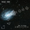 |
Fig. 1. Finding chart for NGC 300. The eight HST fields used in this study are marked on the Digitized Sky Survey image. The shaded area indicates the region we used to derive the integrated light profile from the Spitzer 3.6 μm data. |
We obtained photometry of resolved stellar objects using the GHOSTS pipeline, which is based on DOLPHOT (Dolphin 2000). After obtaining the raw DOLPHOT output catalogs, we applied photometric cuts to select point sources. Details of the pipeline and data-reduction procedures can be found in our previous papers (Radburn-Smith et al. 2011; Monachesi et al. 2016; Jang et al. 2020). Extensive artificial star tests were carried out to estimate uncertainties and recovery rates of our photometry. We converted the WFC3 and WFPC2 photometric systems to the ACS system using equations in Jang & Lee (2015) and Sirianni et al. (2005), respectively.
3. Results
3.1. Color-magnitude diagrams of resolved stars
In Fig. 2 we display color–magnitude diagrams (CMDs) of stars in the eight HST fields. Shaded regions indicate the CMD bins we defined to select distinct stellar populations: main sequence (MS) and upper helium-burning (HeB) stars, typically younger than 300 Myr (blue region), bright asymptotic giant branch (AGB) stars with ages of 1−3 Gyr (yellow region), and red giant branch (RGB) stars mostly older than 3 Gyr (pink region). The CMDs show a gradual change in stellar populations from inner to outer regions as expected. Fields F1, F2, and F7 in the inner regions contain a large population of young MS and red HeB stars. These features are also visible in F3 at R = 7.4 kpc, but are much weaker in the fields beyond R ≈ 10 kpc.
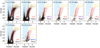 |
Fig. 2. Color-magnitude diagrams of the HST fields along the major (top) and minor (bottom) axes of NGC 300. The field IDs and projected galactocentric distances are marked in each panel. The projected distances for the minor axis fields are corrected for the disk inclination (i = 45°). Blue, yellow, and pink shaded regions represent selection bins for the young (MS and HeB), intermediate-aged (AGB), and old (RGB) stellar populations, respectively. A stellar isochrone for 10 Gyr age with [Fe/H] = −1.6 dex (solid line) and the 50% completeness limit (dashed line) are overlaid in each CMD. |
We detect a significant population of old RGB stars in all the survey fields, indicating that they extend out to at least 18 kpc. The RGB stars show a radial color gradient such that the mean RGB color becomes bluer with increasing radial distance. The narrow sequence of RGB stars in the fields beyond 10 kpc (F4, F5, F6, and F8) matches well with a stellar isochrone of 10 Gyr age with [Fe/H] = −1.6 dex in the Padova models (Bressan et al. 2012) (red line).
The CMDs of NGC 300 exhibit a dense clump of stars at F814W ∼ 26.2 mag, which is the red clump (RC). The weak clustering of stars at F814W ∼ 25.2 mag seen in Fields F5 and F6 is likely the RGB bump. We used these features to estimate the mean stellar age of the galaxy outskirts in Sect. 3.3.
3.2. Radial number density profiles of resolved stars
In Fig. 3, we present the radial star count profiles for the three stellar populations (MS/HeB, AGB, and RGB) along the major (circles) and minor (squares) axes of NGC 300, corrected for the photometric incompleteness using the artificial star data. For the fields that have enough stars (N ≳ 15), we subdivided them into two or three regions to get a better spatial sampling of the radial profile. We measured background levels (shaded regions) using empty fields and provide technical details in Appendix A. Briefly, we used a number of empty fields that are located at a high galactic latitude, similar to the case of the NGC 300 fields. These empty fields are expected to be dominated by foreground stars or unresolved background galaxies. The background level and its uncertainty were taken to be the mean and standard deviation of the source densities in the individual empty fields, respectively.
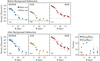 |
Fig. 3. Top: radial star count profiles for the MS/HeB (a), AGB (b), and RGB (c) stars in NGC 300. Circles and squares indicate the profiles along the major and minor axes of the galaxy, respectively. The approximate background levels of each population are marked by shaded regions. Bottom: same as top but after background subtraction. Numbers in each panel indicate field IDs. Dashed lines in panel (d) represent the exponential fit of the major and minor axis profiles. (g) Relative densities of MS/HeB and AGB stars with respect to RGB stars along the major axis. |
In the bottom-left panels of Fig. 3, we plot the background-subtracted radial star counts. The error bars are from Poisson noise of star counts and the background estimation errors. We trace the young stellar populations out to at least 12 kpc along the major axis (left panel). We fit the major and minor axis profiles with an exponential law (dashed lines), resulting in scale lengths for the young stellar component of hd, major = 1.4 ± 0.1 kpc and hd, minor = 1.2 ± 0.1 kpc. While the fit is good along the radially limited minor axis, an exponential model is clearly a poor fit along the major axis.
Both the AGB and RGB star count profiles in panels (e) and (f) show two clear breaks along the major axis: down bending, or Type II break, at R ∼ 6 kpc, and up bending, or Type III break, at R ∼ 8 kpc. The outermost component beyond the Type III break is discussed in Sect. 4.2. Turning our attention towards the minor axis, we find that the sign of a break is not clear, mainly due to the short radial coverage with sparse sampling.
The bottom-right panel of the figure shows the relative number of MS/HeB and AGB stars with respect to RGB stars. The ratio of MS stars becomes very low beyond the Type III break radius, indicating that the outskirts of NGC 300 host substantially less star formation (in a relative sense) than its inner parts. Intriguingly, the ratio of AGB stars to RGB stars tentatively appears to be larger towards NGC 300’s largest major axis radius, although the measurement errors are large.
3.3. Mean age of the NGC 300 outskirts
The absolute magnitude of the RC is known to depend on the age and metallicity of stellar populations (Girardi & Salaris 2001). Three of the eight HST fields around NGC 300 (F4, F5, and F6) show an RC above the 50% completeness level with a dominant old RGB population. These have approximately the same color at the tip of the RGB (TRGB). We generated three groups of artificial stars with ages of 5, 7, and 10 Gyr using the Padova models. Each group contains about two million artificial stars that follow the stellar initial mass function (IMF) of Chabrier (2003). These were shifted according to the distance modulus (m − M)0 = 26.52 ± 0.05 (Dalcanton et al. 2009) and the foreground reddening E(B − V) = 0.011 (Schlafly & Finkbeiner 2011) of NGC 300, and were convolved with photometric uncertainties and incompleteness, similarly to the real stars in the HST fields.
The left three panels of Fig. 4 show the density-coded CMDs (Hess diagrams) of the artificial stars. We adopted metallicities of [Fe/H] = –1.4, –1.5, and –1.6 dex, as marked in the figure, so that all the model CMDs have approximately the same color at the TRGB of (F606W − F814W)TRGB = 1.1. This color is also consistent with those of the observed CMDs. All the model CMDs show a prominent RC. The location of the RC changes gradually with age: F814W ∼ 25.9, ∼26.1, and ∼26.3 mag for the 5-, 7-, and 10-Gyr populations, respectively. There are also two small over-densities above the RC in the 5-Gyr model, which are identified by the AGB bump (at F814W ∼ 25.0 mag) and the RGB bump (at F814W = 25.2 mag). These two bumps almost overlap in the 7-Gyr and 10-Gyr models at F814W ∼ 25.2 mag.
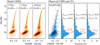 |
Fig. 4. Left three panels: Hess diagrams for the simulated 5, 7, and 10 Gyr simple stellar populations at the distance of NGC 300. The highest density regions of the RC are marked by crosses. We note the gradual change of the RC magnitudes as a function of age. Right four panels: observed CMD of F4, F5, and F6 and its LF (filled histograms) overplotted with the model LFs (open histograms). The red curved line in the CMD represents the stellar isochrone for age = 10 Gyr and [Fe/H] = −1.6 in the Padova models. The probability (P) of the Kolmogorov–Smirnov test for the stars brighter than F814W = 26.5 and 27 mag are marked in the panels with LFs. |
On the right side of Fig. 4, we display a composite CMD of the three observed outer fields (F4, F5, and F6), and its luminosity function (LF) in comparison with the LFs of the model CMDs. The observed LF shows the best match with the 10 Gyr model LF. A Kolmogorov-Smirnov test confirms that the oldest 10 Gyr model is preferred over the other younger models, regardless of the faint boundary of the input stars (F814W = 26.5 and 27.0 mag), indicating that the NGC 300 outskirts are older than 7 Gyr and probably as old as ∼10 Gyr.
3.4. Radial distributions of the RGB stars
In the top panel of Fig. 5 we show the radial density distribution of RGB stars along NGC 300’s major axis. The profile is background subtracted and also corrected for photometric incompleteness, where completeness is mostly higher than 80% except for the inner 5 kpc regions (∼60%). We also plot the integrated light profile we derived from the Spitzer 3.6 μm image using the wedge indicated by the shaded area in Fig. 1 (ϕ = 293° ±22.5°) in order to get a similar spatial sampling with the RGB counts. The integrated light profile was scaled to the RGB density using the Padova stellar models. We generated a well-populated CMD for old (10 Gyr) and low-metallicity ([Fe/H] = –1.6 dex) stars and derived a relation between the 3.6 μm luminosity and the number of RGB stars in the CMD bin.
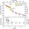 |
Fig. 5. Top: stellar density profile along the NGC 300 major axis. RGB star counts are shown by circles. The orange line with a shaded region indicates the integrated light profile in the Spitzer 3.6 μm band. Surface brightness is shown on the right y-axis, and can be converted to V-mag by adding ∼2.0 mag. Solid lines indicate fits to the resulting three regions using exponential-law models. Also shown is a fit to the outermost component with a power law (dashed line). Bottom: Q-color distribution of the bright RGB stars with F814W ≤ 24.5 mag. Individual stars and their median colors are indicated by gray dots and red circles, respectively. |
The star count and the integrated light profiles overlap in a region between R = 2 and 5 kpc. The two independent profiles show a slight offset of ∼0.5 mag in the inner region. Such an offset is naturally expected as the younger stellar populations in this radial range will contribute to the integrated light. We divided the profile into three components based on the two breaks and fit each component with an exponential-law model. Derived scale lengths (fitting range) for the inner to outer components are: hd, inner = 1.4 ± 0.1 kpc (1 < R [kpc] ≤5), hd, middle = 0.7 ± 0.1 kpc (6 < R [kpc] ≤8), and hd, outer = 3.2 ± 0.5 kpc (9 < R [kpc] ≤19). The fit for the inner component was made using the integrated light only, while that for the middle one is based on both the integrated light and star count data, taking into account their uncertainties. The fits appear to be stable; changing the fitting range of each component by ±1 kpc gives statistically consistent results within 1σ level. When we fit the inner component using the star count data, we find hd, inner = 1.9 ± 0.1 kpc. The break radii are identified at R ∼ 5.9 kpc (Type II) and 8.3 kpc (Type III).
We selected the bright RGB stars with F814W ≤ 24.5 mag and derived the radial color profile, as shown in the bottom panel of Fig. 5. The equivalent color of the RGB at F814W = 23.0 mag, accounting for the slope of the RGB following Monachesi et al. (2013) (Q-index), was used to get the median color with a lower scatter. The color profile shows a gradual decrease out to R ∼ 8 kpc, where the Type III break was detected in the density profile. Beyond the 8 kpc radius, the color profile does not show a measurable gradient and converges to (F606W − F814W)0 = 1.02 ± 0.04. The error budget includes systematic uncertainty due to photometric calibration. We can convert this median color to metallicity using the relation by Streich et al. (2014) with [α/Fe] = 0.3, which results in ![Mathematical equation: $ \rm[Fe/H] = -1.6^{+0.2}_{-0.4} $](/articles/aa/full_html/2020/08/aa38651-20/aa38651-20-eq2.gif) dex.
dex.
4. Discussion
4.1. Comparison with previous studies
Studies of the NGC 300 outskirts have a long history. Early work by de Vaucouleurs & Page (1962) and Carignan (1985) using photographic plates reported that its luminosity profile falls exponentially down to μB ∼ 26 mag arcsec−2. Their profiles, averaged over azimuthal angle, reached out to R ∼ 13′, which is still one of the largest radial extents taken from integrated light. However, in addition to the global exponential fall off, these latter authors also noted slight variations in the profiles. de Vaucouleurs & Page (1962) stated that “The steeper slope beyond r* ∼ 10′ may or may not be real”. A similar profile steepening is also seen in Fig. 14 of Carignan (1985). More recent studies with CCDs presented an integrated light profile of NGC 300 (Kim et al. 2004; Muñoz-Mateos et al. 2007; Laine et al. 2016). However, those ended at R = 9′−10′, making it difficult to discuss the outer disk properties.
Bland-Hawthorn et al. (2005) used resolved star counts from Gemini/GMOS combined with the integrated light from Carignan (1985), finding that NGC 300’s light profile is well described by a single exponential law out to R ∼ 24′ (14 kpc). However, they only had images in one passband (r′) and no other information (e.g., on stellar populations) could be derived. They revisited NGC 300 in Vlajić et al. (2009) with multi-band (g′ and i′) observations using the same instrument; it was confirmed again that the stellar density profile is well approximated by a single exponential law. Vlajić et al. (2009) also derived the metallicity profile of the RGB stars showing a monotonic decrease to  and a flattening or an upturn thereafter, with a mean metallicity of the outer component of [Fe/H] ∼ −1.0 dex.
Our result can be contrasted with the above two studies based on ground-based resolved star counts. Our stellar density profile reaches out to R ∼ 32′ (19 kpc), or about 30% farther than those previous studies, and shows two measurable breaks. The median metallicity of the outer component we derived is ![Mathematical equation: $ \rm[Fe/H] = -1.6^{+0.2}_{-0.4} $](/articles/aa/full_html/2020/08/aa38651-20/aa38651-20-eq4.gif) dex, which is significantly lower than the value by Vlajić et al. (2009). However, the HST fields used in this work are placed along the opposite side (northwest) of NGC 300’s major axis to the GMOS fields used in the previous studies (southeast), which makes it difficult to compare the density profiles directly. The measurable difference in both the density profile and abundance could be due to the asymmetric distribution of the NGC 300 outskirts or different analysis methods applied in each study (e.g., stellar model, background estimation), but the exact origin is unclear and requires further study.
dex, which is significantly lower than the value by Vlajić et al. (2009). However, the HST fields used in this work are placed along the opposite side (northwest) of NGC 300’s major axis to the GMOS fields used in the previous studies (southeast), which makes it difficult to compare the density profiles directly. The measurable difference in both the density profile and abundance could be due to the asymmetric distribution of the NGC 300 outskirts or different analysis methods applied in each study (e.g., stellar model, background estimation), but the exact origin is unclear and requires further study.
Hillis et al. (2016) studied the young stellar disk of NGC 300 using the same HST data as in our fields F3–F6. Using a CMD fitting technique, they isolated a stellar population younger than 200 Myr and found an unbroken young disk profile out to R = 11 kpc (with an upper limit out to 14 kpc) with a scale length of hd = 1.4 ± 0.1 kpc. While the global exponential decay of the young density profile is reproduced in this study, the profile appears to be a poor fit with a single exponential law over the whole radial extent (Fig. 3, bottom left).
The Type II break we find at R ∼ 10′ in the AGB and RGB profiles is also supported by a down bending in the UV profile of NGC 300 found by Roussel et al. (2005) and Gil de Paz et al. (2007). Taken at face value, the youngest stellar disk of the galaxy is also likely truncated.
4.2. Identification of the outer stellar component: extended disk or stellar halo?
The outer stellar component beyond the up bending is well separated from the inner ones in terms of both its stellar density and its stellar populations. The identification of this outer component, as either an extended stellar disk or a stellar halo, is important to understand the growth history of the galaxy outskirts. Unfortunately, it is not easy to distinguish between both options based on the limited information we have, especially with the lack of measurements along the minor axis of the galaxy.
Interpreting the outer component as disk stars, we note that NGC 300 has an extended HI disk reaching out to at least R ∼ 20 kpc (Westmeier et al. 2011), which may be the source of our younger population reaching out to R ∼ 17 kpc. Explaining the upturn in the NGC 300’s outer stellar component is then still hard to explain as it consists mainly of old stars, which would be hard to transport to these extreme radii by the radial migration of earlier disk stars alone. Minchev et al. (2012) used N-body tree-SPH simulations to show that a combination of Type II + III breaks, as found here, can result from gas accretion in the outer region, which has the effect of strongly increasing the eccentricity of the orbits of the existing stellar population beyond Type III (see their Fig. 17). The anti-truncation can also result from the perturbation of a minor merger provided the existence of a gas-rich disk (Younger et al. 2007). A successful NGC 300 disk model should be able to explain both the double break in the density profile and the old stars with a flat color/metallicity profile beyond the Type III break.
Alternatively, the outermost component could be a stellar halo; fitting a power-law model to this (curved dashed line in Fig. 5) resulted in a 2D density slope of αmajor = −4.2 ± 0.5, which is in good agreement with −5.3 ≤ αmajor ≤ −2.7, which was measured for the stellar halos of nearby Milky Way mass disk galaxies (Harmsen et al. 2017). Numerically integrating the power-law profile from 10 kpc to 19 kpc, we obtained an observed total stellar mass of Mhalo, 10−19 = 3 × 10⁷ M⊙. Here we assumed 10 Gyr age with [Fe/H] = −1.6 dex. Combining the halo mass with the total stellar mass of NGC 300 of Mgal = 2 × 10⁹ M⊙ (Muñoz-Mateos et al. 2015; Laine et al. 2016), we obtain the stellar halo mass fraction, Mhalo, 10−19/Mgal = 1.5%. Extrapolating this observed halo profile further inward, the total stellar halo mass fraction becomes several times larger. Such a massive stellar halo would be very unusual in current low-mass disk galaxy models, as low-mass galaxies are assembled from lower-mass dark matter halos with lower star formation efficiency (Purcell et al. 2008; Cooper et al. 2013).
5. Closing remarks
The nearby galaxy NGC 300 has been presented in the literature as a prototypical example of a Type I disk galaxy with a pure exponential light profile over many disk scale lengths. Most exponential disk formation models have difficultly explaining such an extended stellar disk; accordingly we investigated NGC 300’s light distribution using high-resolution HST data in the archive.
We constructed density profiles of different stellar populations reaching out to ∼19 kpc from the galaxy center. We found that the profiles for the AGB and RGB populations show two clear breaks: one down-bending (Type II) at R ∼ 5.9 kpc, and another up-bending (Type III) at R ∼ 8.3 kpc. The stellar populations beyond the Type III break radius become predominantly old (≳9 Gyr) and metal poor ([Fe/H] = –1.6), well separated from the inner disk regions.
While our results cast doubt on the currently established wisdom that NGC 300 is a pure exponential disk galaxy, a more detailed study should be carried out. It is expected that wide-field imaging with large ground-based telescopes would be useful to map out the global structure of the extended stellar component, providing evidence to the formation history of NGC 300.
Acknowledgments
We are thankful to the anonymous referee for his/her useful comments. I.S.J. and R.dJ. gratefully acknowledge support from the Deutsches Zentrum für Luft- und Raumfahrt (DLR) through grant 50OR1815. A.S. acknowledges support for this work by the National Science Foundation Graduate Research Fellowship Program under grant No. DGE 1256260. Any opinions, findings, and conclusions or recommendations expressed in this material are those of the author(s) and do not necessarily reflect the views of the National Science Foundation. This paper is based on observations made with the NASA/ESA Hubble Space Telescope, obtained from the data archive at the Space Telescope Science Institute. STScI is operated by the Association of Universities for Research in Astronomy, Inc. under NASA contract NAS 5-26555. I.S.J. is grateful to Florian Niederhofer for his help in Python programming. AM acknowledges financial support from FONDECYT Regular 1181797 and funding from the Max Planck Society through a Partner Group grant. This research has made use of the NASA/IPAC Extragalactic Database (NED), which is funded by the National Aeronautics and Space Administration and operated by the California Institute of Technology.
References
- Barton, I. J., & Thompson, L. A. 1997, AJ, 114, 655 [Google Scholar]
- Bland-Hawthorn, J., Vlajić, M., Freeman, K. C., & Draine, B. T. 2005, ApJ, 629, 239 [Google Scholar]
- Bressan, A., Marigo, P., Girardi, L., et al. 2012, MNRAS, 427, 127 [NASA ADS] [CrossRef] [Google Scholar]
- Carignan, C. 1985, ApJS, 58, 107 [Google Scholar]
- Chabrier, G. 2003, PASP, 115, 763 [Google Scholar]
- Cooper, A. P., D’Souza, R., Kauffmann, G., et al. 2013, MNRAS, 434, 3348 [Google Scholar]
- Dalcanton, J. J., Williams, B. F., Seth, A. C., et al. 2009, ApJS, 183, 67 [Google Scholar]
- de Vaucouleurs, G., & Page, J. 1962, ApJ, 136, 107 [Google Scholar]
- Dolphin, A. E. 2000, PASP, 112, 1383 [Google Scholar]
- Elmegreen, B. G., & Struck, C. 2016, ApJ, 830, 115 [Google Scholar]
- Erwin, P., Beckman, J. E., & Pohlen, M. 2005, ApJ, 626, L81 [Google Scholar]
- Ferguson, A. M. N., & Clarke, C. J. 2001, MNRAS, 325, 781 [Google Scholar]
- Freeman, K. C. 1970, ApJ, 160, 811 [Google Scholar]
- Gil de Paz, A., Boissier, S., Madore, B. F., et al. 2007, ApJS, 173, 185 [Google Scholar]
- Girardi, L., & Salaris, M. 2001, MNRAS, 323, 109 [Google Scholar]
- Harmsen, B., Monachesi, A., Bell, E. F., et al. 2017, MNRAS, 466, 1491 [Google Scholar]
- Hillis, T. J., Williams, B. F., Dolphin, A. E., Dalcanton, J. J., & Skillman, E. D. 2016, ApJ, 831, 191 [Google Scholar]
- Jang, I. S., & Lee, M. G. 2015, ApJ, 807, 133 [Google Scholar]
- Jang, I. S., de Jong, R. S., Holwerda, B. W., et al. 2020, A&A, 637, A8 [EDP Sciences] [Google Scholar]
- Kennicutt, R. C. 1989, ApJ, 344, 685 [Google Scholar]
- Kim, S. C., Sung, H., Park, H. S., & Sung, E.-C. 2004, Ch. J. Astron. Astrophys, 4, 299 [Google Scholar]
- Laine, J., Laurikainen, E., & Salo, H. 2016, A&A, 596, A25 [NASA ADS] [CrossRef] [EDP Sciences] [Google Scholar]
- Minchev, I., Famaey, B., Quillen, A. C., et al. 2012, A&A, 548, A126 [NASA ADS] [CrossRef] [EDP Sciences] [Google Scholar]
- Monachesi, A., Bell, E. F., Radburn-Smith, D. J., et al. 2013, ApJ, 766, 106 [Google Scholar]
- Monachesi, A., Bell, E. F., Radburn-Smith, D. J., et al. 2016, MNRAS, 457, 1419 [Google Scholar]
- Muñoz-Mateos, J. C., Gil de Paz, A., Boissier, S., et al. 2007, ApJ, 658, 1006 [Google Scholar]
- Muñoz-Mateos, J. C., Sheth, K., Regan, M., et al. 2015, ApJS, 219, 3 [Google Scholar]
- Purcell, C. W., Bullock, J. S., & Zentner, A. R. 2008, MNRAS, 391, 550 [Google Scholar]
- Radburn-Smith, D. J., de Jong, R. S., Seth, A. C., et al. 2011, ApJS, 195, 18 [Google Scholar]
- Roussel, H., Gil de Paz, A., Seibert, M., et al. 2005, ApJ, 632, 227 [NASA ADS] [CrossRef] [Google Scholar]
- Schlafly, E. F., & Finkbeiner, D. P. 2011, ApJ, 737, 103 [NASA ADS] [CrossRef] [Google Scholar]
- Sirianni, M., Jee, M. J., Benítez, N., et al. 2005, PASP, 117, 1049 [Google Scholar]
- Streich, D., de Jong, R. S., Bailin, J., et al. 2014, A&A, 563, A5 [NASA ADS] [CrossRef] [EDP Sciences] [Google Scholar]
- van der Kruit, P. C. 1987, A&A, 173, 59 [NASA ADS] [Google Scholar]
- Vlajić, M., Bland-Hawthorn, J., & Freeman, K. C. 2009, ApJ, 697, 361 [Google Scholar]
- Weiner, B. J., Sellwood, J. A., & Williams, T. B. 2001, ApJ, 546, 931 [Google Scholar]
- Westmeier, T., Braun, R., & Koribalski, B. S. 2011, MNRAS, 410, 2217 [Google Scholar]
- Younger, J. D., Cox, T. J., Seth, A. C., et al. 2007, ApJ, 670, 269 [Google Scholar]
Appendix A: Contamination estimation
NGC 300 is located at a high galactic latitude of b ∼ 79.4° in the sky, and its CMDs shown in Fig. 2 exhibit a well-defined sequence of old RGB stars, indicating that the detected point sources are mostly the NGC 300 stars. Nevertheless, there could be a small contribution of contaminating sources that passed the GHOSTS culls, such as foreground stars in the Milky Way and unresolved background galaxies. These sources should be properly taken into account to derive the intrinsic radial number density profile of the NGC 300 stars. Here we describe the method that we used to measure the contamination levels of the NGC 300 data.
We selected eight fields in empty sky regions taken with each HST instrument used in this study (ACS/WFC, WFC3/UVIS, and WFPC2), as listed in Table A.1. These fields are located at high galactic latitude with |b|≳40°, and also well away from known stellar objects in the sky (e.g., bright stars, star clusters, tidal streams in the Milky Way halo, bright galaxies, and galaxy clusters). The fields for ACS/WFC and WFC3/UVIS have also been used for the background control of M101 in our previous study (Jang et al. 2020). Table A.1 also lists the NGC 300 fields used in this study for reference.
We treated these empty sky fields identically to the NGC 300 fields, deriving point source photometry using the GHOSTS pipeline. Figures A.1–A.3 show CMDs of the emtpy fields taken with ACS/WFC, WFC3/UVIS, and WFPC2, respectively. Shaded regions in the figures indicate the population bins (Ms/HeB, AGB, and RGB) used for the NGC 300 data. The sources presented in the CMDs are considered to be the contaminating sources, either foreground stars or unresolved background galaxies. We calculated the spatial number densities of these sources considering the photometric incompleteness and the effective field area, as listed in Table A.2. Here the errors are taken to be the standard deviation of the individual densities. We used these values to correct for the contribution of contaminating sources in the NGC 300 profiles.
Summary of HST data of the control fields and NGC 300 used in this study
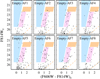 |
Fig. A.1. Color-magnitude diagrams for the selected point sources in the eight empty fields taken with ACS/WFC. We correct for the foreground extinction toward each field using the values in Schlafly & Finkbeiner (2011). Shaded regions are the same as those in Fig. 2. Dashed lines represent the 50% completeness limits. |
Estimated contamination levels for distinct stellar populations measured from the control fields.
All Tables
Estimated contamination levels for distinct stellar populations measured from the control fields.
All Figures
|
Fig. 1. Finding chart for NGC 300. The eight HST fields used in this study are marked on the Digitized Sky Survey image. The shaded area indicates the region we used to derive the integrated light profile from the Spitzer 3.6 μm data. |
| In the text | |
|
Fig. 2. Color-magnitude diagrams of the HST fields along the major (top) and minor (bottom) axes of NGC 300. The field IDs and projected galactocentric distances are marked in each panel. The projected distances for the minor axis fields are corrected for the disk inclination (i = 45°). Blue, yellow, and pink shaded regions represent selection bins for the young (MS and HeB), intermediate-aged (AGB), and old (RGB) stellar populations, respectively. A stellar isochrone for 10 Gyr age with [Fe/H] = −1.6 dex (solid line) and the 50% completeness limit (dashed line) are overlaid in each CMD. |
| In the text | |
|
Fig. 3. Top: radial star count profiles for the MS/HeB (a), AGB (b), and RGB (c) stars in NGC 300. Circles and squares indicate the profiles along the major and minor axes of the galaxy, respectively. The approximate background levels of each population are marked by shaded regions. Bottom: same as top but after background subtraction. Numbers in each panel indicate field IDs. Dashed lines in panel (d) represent the exponential fit of the major and minor axis profiles. (g) Relative densities of MS/HeB and AGB stars with respect to RGB stars along the major axis. |
| In the text | |
|
Fig. 4. Left three panels: Hess diagrams for the simulated 5, 7, and 10 Gyr simple stellar populations at the distance of NGC 300. The highest density regions of the RC are marked by crosses. We note the gradual change of the RC magnitudes as a function of age. Right four panels: observed CMD of F4, F5, and F6 and its LF (filled histograms) overplotted with the model LFs (open histograms). The red curved line in the CMD represents the stellar isochrone for age = 10 Gyr and [Fe/H] = −1.6 in the Padova models. The probability (P) of the Kolmogorov–Smirnov test for the stars brighter than F814W = 26.5 and 27 mag are marked in the panels with LFs. |
| In the text | |
|
Fig. 5. Top: stellar density profile along the NGC 300 major axis. RGB star counts are shown by circles. The orange line with a shaded region indicates the integrated light profile in the Spitzer 3.6 μm band. Surface brightness is shown on the right y-axis, and can be converted to V-mag by adding ∼2.0 mag. Solid lines indicate fits to the resulting three regions using exponential-law models. Also shown is a fit to the outermost component with a power law (dashed line). Bottom: Q-color distribution of the bright RGB stars with F814W ≤ 24.5 mag. Individual stars and their median colors are indicated by gray dots and red circles, respectively. |
| In the text | |
|
Fig. A.1. Color-magnitude diagrams for the selected point sources in the eight empty fields taken with ACS/WFC. We correct for the foreground extinction toward each field using the values in Schlafly & Finkbeiner (2011). Shaded regions are the same as those in Fig. 2. Dashed lines represent the 50% completeness limits. |
| In the text | |
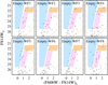 |
Fig. A.2. Same as Fig. A.1, but for WFC3/UVIS fields. |
| In the text | |
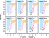 |
Fig. A.3. Same as Fig. A.1, but for WFPC2 fields. |
| In the text | |
Current usage metrics show cumulative count of Article Views (full-text article views including HTML views, PDF and ePub downloads, according to the available data) and Abstracts Views on Vision4Press platform.
Data correspond to usage on the plateform after 2015. The current usage metrics is available 48-96 hours after online publication and is updated daily on week days.
Initial download of the metrics may take a while.