| Issue |
A&A
Volume 640, August 2020
|
|
|---|---|---|
| Article Number | L13 | |
| Number of page(s) | 12 | |
| Section | Letters to the Editor | |
| DOI | https://doi.org/10.1051/0004-6361/202038571 | |
| Published online | 10 August 2020 | |
Letter to the Editor
Detection of vibrationally excited HC7N and HC9N in IRC +10216⋆
1
Grupo de Astrofísica Molecular, Instituto de Física Fundamental (IFF-CSIC), C/ Serrano 121, 28006 Madrid, Spain
e-mail: This email address is being protected from spambots. You need JavaScript enabled to view it.
2
Centro de Desarrollos Tecnológicos, Observatorio de Yebes (IGN), 19141 Yebes, Guadalajara, Spain
3
Department of Space, Earth and Environment, Chalmers University of Technology, Onsala Space Observatory, 439 92 Onsala, Sweden
4
Observatorio Astronómico Nacional (OAN, IGN), Madrid, Spain
5
Institut de Radioastronomie Millimétrique, 300 Rue de la Piscine, 38406 Saint Martin d’Hères, France
Received:
3
June
2020
Accepted:
29
June
2020
Abstract
Observations of IRC +10216 with the Yebes 40 m telescope between 31 and 50 GHz have revealed more than 150 unidentified lines. Some of them can be grouped into a new series of 26 doublets, harmonically related with integer quantum numbers ranging from Jup = 54 to 80. The separation of the doublets increases systematically with J, that is to say, as expected for a linear species in one of its bending modes. The rotational parameters resulting from the fit to these data are B = 290.8844 ± 0.0004 MHz, D = 0.88 ± 0.04 Hz, and q = 0.1463 ± 0.0001 MHz. The rotational constant is very close to that of the ground state of HC9N. Our ab initio calculations show an excellent agreement between these parameters and those predicted for the lowest energy vibrationally excited state, ν19 = 1, of HC9N. This is the first detection, and complete characterization in space, of vibrationally excited HC9N. An energy of 41.5 cm−1 is estimated for the ν19 state. In addition, 17 doublets of HC7N in the ν15 = 1 state, for which laboratory spectroscopy is available, were detected for the first time in IRC +10216. Several doublets of HC5N in its ν11 = 1 state were also observed. The column density ratio between the ground and the lowest excited vibrational states are ≈127, 9.5, and 1.5 for HC5N, HC7N, and HC9N, respectively. We find that these lowest-lying vibrational states are most probably populated via infrared pumping to vibrationally excited states lying at ≈600 cm−1. The lowest vibrationally excited states thus need to be taken into account to precisely determine absolute abundances and abundance ratios for long carbon chains. The abundance ratios N(HC5N)/N(HC7N) and N(HC7N)/N(HC9N) are 2.4 and 7.7, respectively.
Key words: molecular data / line: identification / stars: carbon / circumstellar matter / stars: individual: IRC +10216 / astrochemistry
Based on observations carried out with the Yebes 40 m telescope and the IRAM 30 m telescope. The 40 m radiotelescope at Yebes Observatory is operated by the Spanish Geographic Institute (IGN, Ministerio de Transportes, Movilidad y Agenda Urbana). IRAM is supported by INSU/CNRS (France), MPG (Germany), and IGN (Spain).
© ESO 2020
1. Introduction
Sensitive line surveys are the best tool to unveil the molecular content of astronomical sources and to search for new molecules. A key element for carrying out a detailed analysis of line surveys is the availability of spectroscopic information of the already-known species, their isotopologues, and their vibrationally excited states. The ability to identify the maximum possible number of lines coming from them leaves the cleanest possible forest of unidentified lines; this opens up a chance to discover new molecules and to get insights into the chemistry and chemical evolution of the observed object. Lines from vibrationally excited states of long molecules have been observed in the carbon-rich circumstellar envelope (CSE) IRC +10216; C4H and C6H are good examples of such emission (Guélin et al. 1993; Yamamoto et al. 1987; Cernicharo et al. 2008). The longer a linear molecule is, the lower in energy its vibrational bending modes are. Hence, even in relatively cold regions of CSEs, the lines from vibrationally excited states can be rather prominent in sensitive surveys. Moreover, the correct determination of the abundance ratios between species of the same family (e.g. CnH radicals or cyanopolyynes HC2n + 1N) requires an estimation of populations in vibrationally excited states if they are significant.
Rotational lines from vibrationally excited levels of moderate energies provide useful information on the pumping mechanisms in the CSE and allow us to assess the role of infrared (IR) pumping and its effect on intensity line variations with the stellar phase (Cernicharo et al. 2008, 2014; Agúndez et al. 2017; Pardo et al. 2018). A different case occurs when these lines involve very high energy vibrational states because they trace the physical and chemical conditions of the innermost and warm regions of CSEs. The main difference between the rotational lines from low and high energy vibrational states relies on the line profile. Transitions from low energy excited vibrational levels should show the same velocity extent and similar line profiles as those of the ground vibrational state, with C4H and C6H as clear examples (Guélin et al. 1993; Cernicharo et al. 2008). However, rotational lines from high energy excited vibrational states show Gaussian profiles and trace the kinematics of the gas in the innermost regions (Cernicharo et al. 2011, 2013; Patel et al. 2011).
In this Letter we report on the discovery of a new series of lines toward IRC +10216 that we attribute to the ν19 = 1 state of HC9N, for which we determine accurate rotational constants. In addition, we report on the detection of HC7N in the ν15 = 1 and ν15 = 2 states, and of HC5N in the ν11 = 1 state. The abundance ratio between members of this molecular family is revisited in the light of the high column densities observed in vibrationally excited states for some of them.
2. Observations
The Q-band observations (31.0–50.3 GHz) were carried out in spring 2019 with the 40 m radiotelescope of the Centro Astronómico de Yebes (IGN, Spain), hereafter Yebes 40 m. New receivers, built within the Nanocosmos project1 and installed at the telescope, were used for these observations during its commissioning phase. The experimental setup will be described elsewhere (Tercero et al., in prep.). Briefly, the Q-band receiver consists of two HEMT cold amplifiers covering the 31.0–50.3 GHz band with horizontal and vertical polarizations. Receiver temperatures vary from 22 K at 32 GHz to 42 K at 50 GHz. The backends are 16 × 2.5 GHz fast Fourier transform spectrometers (FFTS) with a spectral resolution of 38.1 kHz providing the whole coverage of the Q-band in both polarizations. The observing mode was position switching with an off position at 300″ in azimuth. The main beam efficiency varies from 0.6 at 32 GHz to 0.43 at 50 GHz. The spectra were smoothed to a resolution of 0.195 MHz, that is, a velocity resolution of ≈1.9 and 1.2 km s−1 at 31 and 50 GHz, respectively. The sensitivity of the final spectra varies from 0.4 to 1 mK across the Q-band, which is a factor of ≈10 better than previous observations in the same band made with the Nobeyama 45 m telescope (Kawaguchi et al. 1995).
The observations in the λ3 mm band presented in this paper were carried out with the IRAM 30 m radio telescope and were described in detail by Cernicharo et al. (2019). Briefly, they correspond to observations acquired over the last 35 years and cover the 70–116 GHz domain with very high sensitivity (1–3 mK). Examples of these data can be found in Cernicharo et al. (2004, 2007, 2008, 2019) and Agúndez et al. (2008, 2014).
The beam size of the Yebes 40 m in the Q-band is in the range 36–56″, while that of the IRAM 30 m telescope in the 3 mm domain is 21–30″. Pointing corrections were obtained by observing strong nearby quasars and the SiO masers of R Leo. Pointing errors were always within 2–3″. The intensity scale, antenna temperature ( ), was corrected for atmospheric absorption using the ATM package (Cernicharo 1985; Pardo et al. 2001). We adopted calibration uncertainties to be 10%. Additional uncertainties could arise from the line intensity fluctuation with time, induced by the variation of the stellar IR flux (Cernicharo et al. 2014; Pardo et al. 2018). All data were analyzed using the GILDAS package2.
3. Results
One of the most surprising results from the line survey in the Q-band is the presence of bright lines from vibrationally excited states of C4H, C6H, HC5N, and HC7N, and of two series of doublets recently assigned by Cernicharo et al. (2019) to MgCCCN and MgCCCCH (see Fig. 1, where the bottom panel shows one of the MgCCCN doublets). Also, a new series of lines consisting of 26 doublets, with central frequencies in harmonic relation from J = 54 up to J = 80, was found in the Q-band data.
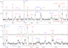 |
Fig. 1. Data from two frequency ranges within the Q-band observed with the Yebes 40 m telescope towards IRC +10216. Each frequency range is shown through two panels with different limits in intensity. The vertical scale is antenna temperature in mK. The horizontal scale is the rest frequency in MHz. Labels for HC7N features are in blue, while those belonging to HC9N are in violet. Other spectral features from known species, together with unidentified lines (labeled as “U” lines), are indicated in red. The N = 16−15 doublet of MgCCCN, a new species recently detected (Cernicharo et al. 2019), is shown in the bottom panels. Vibrationally excited lines from HC7N, HC9N, and C6H are nicely detected at these frequencies. Additional lines from vibrationally excited states of HC5N, HC7N, and HC9N are shown in Figs. 2, A.1, and A.3. |
None of the frequencies of the new doublets could be identified in the public JPL (Pickett et al. 1998) or CDMS (Müller et al. 2005) catalogs or in the MADEX catalog (Cernicharo 2012). They belong to a new molecular species or to a new vibrationally excited state of a known molecule. The lines appear at frequencies slightly higher than those of HC9N with the same quantum numbers. Line frequencies for this series of doublets were determined by fitting them with a specific line profile typical of expanding envelopes (Cernicharo et al. 2018). Selected lines of this series are shown in Figs. 1 and 2. The typical profile of the lines with rather sharp edges allows us to fit the lines’ central frequencies with an accuracy on the order of, or even better than, the spectral resolution of the data, even when signals are weak (Cernicharo et al. 2018). Some doublets of this series are blended with other features, but frequencies can still be derived for most of them by fixing the expanding velocity to 14.5 km s−1 (Cernicharo et al. 2000, 2018). However, the integrated line intensities are rather uncertain in these cases. Observed and fitted line frequencies for these doublets are given in Table A.2. One of the components of the J = 64−63 doublet is fully blended with HC7N J = 33−32, with a frequency difference between both features of ≈0.5 MHz. The other component of the same transition is blended with HCCC13CCN J = 14−13, with a frequency difference of 1.3 MHz. This is the only doublet missing in the series from J = 54−53 through J = 80−79.
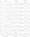 |
Fig. 2. Selected doublets of HC9N ν19 = 1 in the 31–50 GHz domain. Left panels: lines of HC9N in the ground vibrational state. The rotational quantum numbers are indicated in the top-right side of each panel. The same transitions for the ν19 = 1 state are shown in the middle (e component) and right (f component) panels. The intensity scale is antenna temperature in mK. The abscissa corresponds to local standard of rest (LSR) velocities in km s−1. The vertical violet dotted line at −26.5 km s−1 indicates the systemic velocity of the envelope (Cernicharo et al. 2000, 2018). Two additional ν19 doublets are shown in Fig. 1. |
The line frequencies were fitted to the following expression for the energy of the rotational levels in a excited vibrational bending mode with ℓ = 1:
 (1)
(1)
where the sign ± corresponds to the different parities of each doublet (f for + and e for −, assuming qt is positive following the convection of Brown et al. 1975) for a given value of J. Additional distortion terms were found unnecessary in the fitting process, the results of which are: B = 290.8844 ± 0.0003 MHz, D = 0.88 ± 0.04 Hz and qt = 0.1463 ± 0.0001 MHz, where the quoted uncertainties are 1 σ values. The standard deviation of the fit to the 52 observed lines is 105 kHz (roughly half a resolution element). The rotational constant, B, is just 0.37 MHz larger than that of the ground state of HC9N, while the distortion constant, D, is practically the same: for the ground state of HC9N, B = 290.51832 ± 0.00001 MHz and D = 0.860 ± 0.010 Hz (McCarthy et al. 2000). Hence, it is very likely that this series of doublets corresponds to a vibrational state of HC9N with an excited bending mode. From the observed value of qt and B, it is possible to estimate the frequency of this bending mode using the relation ων≈ 2.6  cm−1 (Gordy & Cook 1984). To assign the lines to one of the bending modes of HC9N, we performed ab initio calculations at different levels of theory (see Appendix B). We unambiguously conclude that the lines belong to the lowest energy bending mode, ν19 = 1, of HC9N. From the observed rotational constants, we derive a first order vibration-rotation coupling constant α19 = −0.3661 ± 0.0004 MHz. Line intensities and other parameters for the observed HC9N lines in the ground and its ν19 states are given in Table A.2.
For HC5N, in addition to the lines of the ground vibrational state, all the doublets arising from its lowest vibrationally excited state ν11 were detected in the 31–50 and 70–116 GHz domains. It had previously been detected toward CRL 618 (Cernicharo et al. 2001; Wyrowski et al. 2003). Its energy above the ground state was estimated by Vichietti & Haiduke (2012) to be ≈111 cm−1 (see also Appendix B). Details on the available laboratory spectroscopy for this bending mode of HC5N are given in Appendix A. Selected lines are shown in Fig. A.1, and the derived parameters are given in Table A.4.
For HC7N, two series of lines from the ν15 and 2ν15 were detected in addition to those from the ground vibrational state. Figure 1 shows a couple of doublets from these two vibrationally excited states. Additional lines are shown in Fig. A.3. In the 70–116 GHz domain, only lines from the ν15 state up to Jup = 72 were detected. Line parameters for HC7N are given in Table A.3. This is the first time that this state has been analyzed in detail in space. Nevertheless, the ν15 and 2ν15 states are reported, but not discussed, in the figures in Pardo et al. (2004, 2008); Pardo & Cernicharo (2007). Several unidentified features in the 1.3 cm line survey of IRC +10216 by Gong et al. (2015) can also be assigned to the ν15 state of HC7N, namely U21458.8 (J = 19−18e), U23732.7 (J = 21−20f), U24862.7 (J = 22−21f), U25976.2, and U25992.8 (J = 23−22e and f components).
4. Discussion
Vibrationally excited cyanopolyynes show a clear trend in which the line intensities, relative to those of the ground vibrational state, increase with increasing chain length. For HC5N, the observed intensity ratio between the ground and the sum of the two components (e and f) of its ν11 = 1 state is ≈30 (see Fig. A.1), while for HC7N and its ν15 = 1 state the ratio is ≈8, and for HC9N and its ν19 = 1 state it is ≈1. From the observed line shapes for these species, and taking into account the half power beam of the two telescopes, the emission arises from the external layers of the envelope where ultraviolet photons drive a rich photochemistry (Agúndez et al. 2017). The kinetic temperature in this zone of the CSE is ≈20-30 K (Agúndez et al. 2017). Hence, it is difficult to believe that the ν11 = 1 state of HC5N, which is at ≈160 K above the ground (Vichietti & Haiduke 2012), is pumped by collisions alone. The same applies to the ν15 = 1 and ν19 = 1 states of HC7N and HC9N, respectively, which lie at ≈92 K (Vichietti & Haiduke 2012) and ≈72 K (this work) above the ground. Pumping through IR photons coming from the internal regions of the envelope probably plays an important role in the excitation of these species.
We analyzed the HC5N, HC7N, and HC9N data by constructing rotational diagrams for their ground and low-lying vibrational states. We assumed a 15″ radius for the source and convolved it with the main beam of both telescopes, depending on the line. For HC9N, we find a rotational temperature for the ν19 = 1 state very similar to that of the ground vibrational state, ≈23.5 K, and a column density ratio between the ground and the ν19 = 1 state of 1.45 ± 0.50 (see Fig. 3). The vibrational partition function at 23.5 K (see Table A.1) is ≈1.15. If the ν19 = 1 state is populated by collisions and thermalized with the ground state at this temperature, then its expected column density would be 8% that of the ground state. In fact, the derived vibrational temperature for the ν19 = 1 is close to 80 K. Hence, an efficient mechanism must exist to pump molecules into this excited vibrational state. The column densities of HC9N in the ground and the ν19 = 1 states are (4.5 ± 0.5)×1013 cm−2 and (3.1 ± 0.5)×1013 cm−2, respectively. The total column density of this species is, hence, (7.6 ± 1.4)×1014 cm−2. We searched for possible lines that could be assigned to the ν19 = 2 state without success. Hence, contribution from other vibrational levels is expected to be marginal.
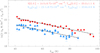 |
Fig. 3. Rotational diagram of HC9N in its ground state (red) and ν19 = 1 vibrationally excited state (blue). The derived rotational temperatures and column densities are indicated in the plot. |
For HC5N and HC7N, the rotational diagram analysis indicates the presence of a cold and a warm regime for the ground and the first vibrationally excited states (see Appendices A.1 and A.2). For these two components of HC5N (Trot ≃ 10 K and 25 K, respectively), we derive N(ground)/N(ν11 = 1)≈127 and 93, respectively (see Appendix A.1). The total column density of HC5N is thus (8.3 ± 0.7)×1014 cm−2, with a negligible contribution of the ν11 state. For the cold (Trot ≃ 17 K) and warm (Trot≃32 K) HC7N components, we derive N(ground)/N(ν15 = 1)≈9.5 and 1.5, respectively (see Appendix A.2). The total column density of HC7N, including the contribution of its ν15 state, is 3.5 ± 0.7 × 1014 cm−2. Hence, N(HC5N)/N(HC7N) ≃ 2.4 and N(HC7N)/N(HC9N) ≃ 7.7. The values obtained for these ratios by Gong et al. (2015), without any correction for the vibrational states, are 1.24 and 14.8, respectively. We note that without the contribution of the ν19 state, the abundance ratio N(HC7N)/N(HC9N) would be a factor of ≃2 higher. The trend in the total abundance ratio between consecutive cyanopolyynes is similar to that found in cold molecular clouds, ≃3–4; however, for long members of this molecular family, the low energy bending modes population can be as high as that of the ground state.
IR pumping for polyatomic molecules can proceed through different paths. Stretching and bending modes harbor a large number of states and bands that provide a plethora of radiative paths to pump the different levels of the molecule. The simple case of the triatomic molecule HNC, which has two stretching modes and one bending mode, was studied by Cernicharo et al. (2014). Excitation through each vibrational mode has a different effect on the line intensities of the ground vibrational state. In the case of HNC, the frequency of the bending mode is high and its IR intensity corresponds to large Einstein coefficients (i.e. the molecule in the bending mode decays mainly to the ground vibrational state). However, for long linear molecules, the frequencies of their bending modes and their IR intensities decrease with increasing chain length. Hence, Einstein coefficients of pure rotational transitions within the bending mode are similar to those of ro-vibrational transitions between the bending mode and the ground vibrational state. This allows for the maintenance of a significant population in the excited bending mode.
While in HNC there are a few radiative paths that redistribute the population of the ground vibrational state between the different vibrationally excited states, in the case of HC9N there are ten stretching and nine bending modes. Hence, the number of transitions from the ground to excited vibrational states and the subsequent radiative de-excitation cascades is huge. Nevertheless, IR pumping will also depend on the flux of the source at the wavelengths of the different IR bands (see, e.g. Fonfría et al. 2008; Agúndez et al. 2017). In the case of IRC +10216, it is well known that the IR emission peaks around 10 μm (Cernicharo et al. 1999). Hence, we could expect to have a dominant path through vibrational bands with large IR intensities and frequencies around 1000 cm−1.
To investigate these effects on the population of the excited vibrational states of cyanopolyynes in IRC +10216, we carried out excitation and radiative transfer calculations for HC5N, HC7N, and HC9N. The physical structure of the envelope and the radial abundance profiles are taken from the chemical model of IRC +10216 from Agúndez et al. (2017). We consider rotational levels within the ground vibrational state, and also within the lowest-lying vibrational state (ν11 = 1 for HC5N, ν15 = 1 for HC7N, and ν19 = 1 for HC9N). In addition, we include for each molecule rotational levels within a vibrational state associated with the CH bending mode (ν7 = 1 for HC5N, ν9 = 1 for HC7N, and ν11 = 1 for HC9N), which has the most intense fundamental band at mid-IR wavelengths, where the radiation field in IRC +10216 is high. We adopted the IR intensities calculated in this work at the second order Møller Plesset perturbation theory (MP2; Møller & Plesset 1934) in the anharmonic limit (see Table B.4). Since IR intensities between excited vibrational states are not known for these molecules, we assumed that molecules from the mid-IR-lying excited vibrational state decay to the lowest-lying vibrational state with the same Einstein coefficient as to the ground vibrational state. We note that this assumption is an important source of uncertainty in the models. We adopted the approximate expression of Deguchi & Uyemura (1984) as rate coefficients for pure rotational excitation through inelastic collisions with H2. We considered ro-vibrational excitation through collisions to be negligible, an assumption that could introduce important uncertainties in the models due to the low energy separation between the rotational levels of the ground and the lowest-lying vibrational states. In summary, IR pumping occurs through absorption in the fundamental band of the CH bending mode, which lies around 600 cm−1 for the three cyanopolyynes, and through further radiative decay to the lowest-lying vibrational states and to the ground state.
In Fig. 4 we show the calculated line profiles for one selected rotational transition of HC5N, HC7N, and HC9N lying in the Q-band in both the ground and the lowest-lying vibrational state. We see that the intensity of the line belonging to the lowest-lying vibrational state approaches the intensity of the line in the ground vibrational state as the size of the cyanopolyyne increases. The calculated line intensity ratio between the ground state and the lowest-lying vibrational state is ∼3.9, ∼2.2, and ∼1.9 for HC5N, HC7N, and HC9N, respectively. These values differ from those observed. For example, they overestimate the relative population of the ν11 = 1 state of HC5N and the ν15 = 1 state of HC7N, although they agree reasonably well for the ν19 = 1 state of HC9N. In any case, the model satisfactorily reproduces the observed trend of increasing relative population of the vibrationally excited state with increasing molecular size.
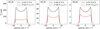 |
Fig. 4. Calculated line profiles for selected lines of HC5N, HC7N, and HC9N in their ground state (G.S.) and lowest energy bending vibrational states. Calculated intensities have been multiplied by 10, 8, and 2 for HC5N, HC7N, and HC9N, respectively, to match the observed intensities of the ground vibrational state lines. |
The observed behavior in the abundance ratio of the cyanopolyynes could introduce an important limitation in detecting longer chains. While HC11N could be present in the envelope, its presence in space has never been confirmed (Cordiner et al. 2017). In our sensitive Q-band data, none of the expected transitions of the ground state are detected. Theoretical calculations of the vibrational modes of this species by Vichietti & Haiduke (2012) suggest that the lowest bending mode, ν23, will be at an energy of 42 K. The effect of IR pumping could be very similar to that of HC9N and would reduce the intensity of the rotational lines of the ground state by a factor of two. Hence, detecting HC11N would be at the sensitivity limit of present instruments. IR pumping also has important consequences on the possibility of detecting other long chain molecules, such as C9H, C10H, and C11H. Their rotational frequencies are well known (see Gottlieb et al. 1998 and references therein). We have searched for them in our Q-band data without success. These species, as is the case for C6H (Cernicharo et al. 2008), have very low energy bending modes that could be highly populated, decreasing the chances of detecting them in their ground vibrational states.
Acknowledgments
The Spanish authors thank Ministerio de Ciencia e Innovación for funding support through project AYA2016-75066-C2-1-P. We also thank ERC for funding through grant ERC-2013-Syg-610256-NANOCOSMOS. MA thanks Ministerio de Ciencia e Innovación for Ramón y Cajal grant RyC-2014-16277. CB thanks Ministerio de Ciencia e Innovación for Juan de la Cierva grant FJCI-2016-27983. LVP acknowledges support from the Swedish Research Council and from the ERC through the consolidator grant 614264.
References
- Agúndez, M., Fonfría, J. P., Cernicharo, J., et al. 2008, A&A, 479, 493 [NASA ADS] [CrossRef] [EDP Sciences] [Google Scholar]
- Agúndez, M., Cernicharo, J., & Guélin, M. 2014, A&A, 570, A45 [NASA ADS] [CrossRef] [EDP Sciences] [Google Scholar]
- Agúndez, M., Cernicharo, J., Quintana-Lacaci, G., et al. 2017, A&A, 601, A4 [NASA ADS] [CrossRef] [EDP Sciences] [Google Scholar]
- Bizzocchi, L., & Esposti, Degli 2004, ApJ, 614, 518 [NASA ADS] [CrossRef] [Google Scholar]
- Botschwina, P., Horn, M., Markey, M., & Oswald, R. 1997, Mol. Phys., 92, 381 [CrossRef] [Google Scholar]
- Brown, J. M., Hougen, J. T., Huber, K.-P., et al. 1975, J. Mol. Spectrosc., 55, 500 [CrossRef] [Google Scholar]
- Cernicharo, J. 1985, Internal IRAM Report (Granada: IRAM) [Google Scholar]
- Cernicharo, J. 2012, in ECLA 2011: Proc. of the European Conference on Laboratory Astrophysics, eds. C. Stehl, C. Joblin, & L. d’Hendecourt (Cambridge: Cambridge Univ. Press), EAS Publ. Ser., 251, https://nanocosmos.iff.csic.es/?page_id=1619 [Google Scholar]
- Cernicharo, J., Yamamura, I., González-Alfonso, E., et al. 1999, ApJ, 526, L41 [NASA ADS] [CrossRef] [PubMed] [Google Scholar]
- Cernicharo, J., Guélin, M., & Kahane, C. 2000, A&AS, 142, 181 [NASA ADS] [CrossRef] [EDP Sciences] [Google Scholar]
- Cernicharo, J., Heras, A. M., Pardo, J. R., et al. 2001, ApJ, 546, L127 [NASA ADS] [CrossRef] [Google Scholar]
- Cernicharo, J., Guélin, M., & Pardo, J. R. 2004, ApJ, 615, L145 [NASA ADS] [CrossRef] [Google Scholar]
- Cernicharo, J., Guélin, M., Agúndez, M., et al. 2007, A&A, 467, L37 [NASA ADS] [CrossRef] [EDP Sciences] [Google Scholar]
- Cernicharo, J., Guélin, M., Agúndez, M., et al. 2008, ApJ, 688, L83 [NASA ADS] [CrossRef] [Google Scholar]
- Cernicharo, J., Agúndez, M., Kakane, C., et al. 2011, A&A, 529, L3 [NASA ADS] [CrossRef] [EDP Sciences] [Google Scholar]
- Cernicharo, J., Daniel, F., Castro-Carrizo, A., et al. 2013, ApJ, 778, L25 [Google Scholar]
- Cernicharo, J., Teyssier, D., Quintana-Lacaci, G., et al. 2014, ApJ, 796, L21 [NASA ADS] [CrossRef] [Google Scholar]
- Cernicharo, J., Guélin, M., Agúndez, M., et al. 2018, A&A, 618, A4 [NASA ADS] [CrossRef] [EDP Sciences] [Google Scholar]
- Cernicharo, J., Cabezas, C., Pardo, J. R., et al. 2019, A&A, 630, L2 [NASA ADS] [CrossRef] [EDP Sciences] [Google Scholar]
- Cooksy, A. L., Gottlieb, C. A., Killian, T. C., et al. 2015, ApJS, 216, 30 [NASA ADS] [CrossRef] [Google Scholar]
- Cordiner, M. A., Charnley, S. B., Kisiel, Z., et al. 2017, ApJ, 850, 187 [NASA ADS] [CrossRef] [Google Scholar]
- Degli Esposti, C., Bizzocchi, L., Botschwina, P., et al. 2005, J. Mol. Spectrosc., 230, 185 [CrossRef] [Google Scholar]
- Deguchi, S., & Uyemura, M. 1984, ApJ, 285, 153 [NASA ADS] [CrossRef] [Google Scholar]
- Fonfría, J. P., Cernicharo, J., Richter, M. J., & Lacy, J. 2008, ApJ, 673, 445 [NASA ADS] [CrossRef] [Google Scholar]
- Frisch, M. J., Trucks, G. W., Schlegel, H. B., et al. 2009, Gaussian 09, Revision D.01 (Wallingford, CT: Gaussian, Inc.) [Google Scholar]
- Gottlieb, C. A., McCarthy, M. C., Travers, M. J., et al. 1998, J. Chem. Phys., 109, 5433 [CrossRef] [Google Scholar]
- Gottlieb, C. A., McCarthy, M. C., & Thaddeus, P. 2010, ApJS, 189, 261 [CrossRef] [Google Scholar]
- Gong, Y., Henkel, C., Spezzano, S., et al. 2015, A&A, 574, A56 [NASA ADS] [CrossRef] [EDP Sciences] [Google Scholar]
- Gordy, W., & Cook, R. 1984, Microwave Molecular Spectra, Techniques of Chemistry (New York: Wiley) [Google Scholar]
- Guélin, M., Cernicharo, J., Navarro, S., et al. 1993, A&A, 182, L37 [Google Scholar]
- Hutchinson, M., Kroto, H. W., & Walton, D. R. M. 1980, J. Mol. Spectrosc., 82, 394 [NASA ADS] [CrossRef] [Google Scholar]
- Iida, M., Ohshima, Y., & Endo, Y. 1991, ApJ, 371, L45 [CrossRef] [Google Scholar]
- Kawaguchi, K., Kasai, Y., Ishikawa, S., & Kaifu, N. 1995, PASJ, 47, 853 [Google Scholar]
- Lee, C., Yang, W., & Parr, R. G. 1988, Phys. Rev. B, 37, 785 [Google Scholar]
- McCarthy, M. C., Levine, E. S., Apponi, A. J., & Thaddeus, P. 2000, J. Mol. Spectrosc., 203, 75 [NASA ADS] [CrossRef] [Google Scholar]
- Møller, C., & Plesset, M. S. 1934, Phys. Rev., 46, 618 [NASA ADS] [CrossRef] [Google Scholar]
- Müller, H. S. P., Schlöder, F., Stutzki, J., & Winnewisser, G. 2005, J. Mol. Struct., 742, 215 [NASA ADS] [CrossRef] [Google Scholar]
- Pardo, J. R., & Cernicharo, J. 2007, ApJ, 654, 978 [NASA ADS] [CrossRef] [Google Scholar]
- Pardo, J. R., Cernicharo, J., & Serabyn, E. 2001, IEEE Trans. Antennas Propag., 49, 12 [NASA ADS] [CrossRef] [MathSciNet] [Google Scholar]
- Pardo, J. R., Cernicharo, J., Goicoechea, J. R., et al. 2004, ApJ, 615, L145 [NASA ADS] [CrossRef] [Google Scholar]
- Pardo, J. R., Cernicharo, J., Goicoechea, J. R., et al. 2008, ApJ, 661, 250 [NASA ADS] [CrossRef] [Google Scholar]
- Pardo, J. R., Cernicharo, J., Velilla-Prieto, L., et al. 2018, A&A, 615, L4 [NASA ADS] [CrossRef] [EDP Sciences] [Google Scholar]
- Patel, N. A., Young, K. H., Gottlieb, C. A., et al. 2011, ApJS, 193, 17 [NASA ADS] [CrossRef] [Google Scholar]
- Pickett, H. M., Poynter, R. L., Cohen, E. A., et al. 1998, J. Quant. Spectrosc. Radiat. Transfer, 60, 883 [Google Scholar]
- Vichietti, R. M., & Haiduke, R. L. A. 2012, Spectrochim. Acta Part A, 90, 1 [CrossRef] [Google Scholar]
- Wyrowski, F., Schilke, P., Thorwirth, S., et al. 2003, ApJ, 586, 344 [NASA ADS] [CrossRef] [Google Scholar]
- Yamada, K. M. T., Degli Esposti, C., Botschwina, P., et al. 2004, A&A, 425, 767 [NASA ADS] [CrossRef] [EDP Sciences] [Google Scholar]
- Yamamoto, S., Saito, S., Guélin, M., et al. 1987, ApJ, 323, L149 [NASA ADS] [CrossRef] [Google Scholar]
Appendix A: Line frequencies
The main goal of this paper is to study the emission from vibrationally excited states of the long cyanopolyynes HC5N, HC7N, and HC9N. However, many lines in the 31–50 GHz and 70–116 GHz frequency ranges arise from the vibrationally excited states of the CnH family of radicals. C4H in its ν7 and 2ν7 states were previously reported in this source (Guélin et al. 1993), and its frequencies are well known from laboratory measurements (Yamamoto et al. 1987; Cooksy et al. 2015). C6H in its ν11 state was detected and spectroscopically characterized in this source (Cernicharo et al. 2008). One of the doublets of this vibrational state of C6H is shown in the top panel of Fig. 1. Additional laboratory information for this state was provided by Gottlieb et al. (2010). Most of these data have already been analyzed and further details will be published elsewhere (Pardo et al., in prep.). The following sections describe the data and the spectroscopic literature used in this work for HC5N and HC7N. We discussed HC9N in Sect. 3, where observed lines are shown in Fig. 2 and observed frequencies are given in Table A.2. All these vibrationally excited states were implemented into the MADEX code (Cernicharo 2012), allowing for the calculation of column densities and the search for all their rotational lines in the 31–50 GHz and 70–116 GHz frequency ranges.
Observed line parameters of HC9N.
To evaluate the fraction of molecules in the different vibrational states for the typical temperatures of the external envelope (10–40 K) of IRC +10216, we calculated the vibrational partition function of these molecules using the standard expression (see, e.g. Gordy & Cook 1984)
 (A.1)
(A.1)
where ωi and gi represent the energy and the degeneracy of each vibrational mode i. For HC9N, we used our ab initio values for the vibrational frequencies (see Appendix B). For HC5N, HC7N, and HC11N, we used the calculations from Vichietti & Haiduke (2012). The results are given in Table A.1.
Vibrational partition function for HC2n + 1N (n = 2 − 5).
For low vibrational temperatures, the value of the vibrational partition function is dominated by the lowest energy vibrational state. In this case
 (A.2)
(A.2)
where ωl and gl are the frequency and the degeneracy of this lowest energy state and Tvib is the vibrational temperature. The abundance ratio between this level (we assume a bending mode, i.e. gl = 2) and the ground state (g = 1) is given by N(νl)/N(ground) ≃2e−(hωl/KTvib), where N(ground) is the column density in the ground state, N(ground) = NT/Qvib, and NT is the total number of molecules in all vibrational states.
For a vibrational temperature of 20 K, and using the frequencies in Table B.4, we obtain
N(HC5N ν11)/N(HC5N ground state) ≃ 0.00,
N(HC7N ν15)/N(HC7N ground state) ≃ 0.04,
N(HC9N ν19)/N(HC9N ground state) ≃ 0.05,
while for a vibrational temperature of 50 K we obtain
N(HC5N ν11)/N(HC5N ground state) ≃ 0.08,
N(HC7N ν15)/N(HC7N ground state) ≃ 0.41,
N(HC9N ν19)/N(HC9N ground state) ≃ 0.46,
that is to say, for a vibrational temperature of 50 K, HC7N and HC9N will have a significant fraction of molecules in their lowest energy bending modes (ν15 and ν19). However, HC5N would need higher vibrational temperatures to have a significant fraction of molecules in its ν11 mode.
A.1. HC5N
For HC5N, the rotational spectrum was measured in the laboratory for several vibrationally excited states involving the ν6, ν7, ν8, ν9, ν10, and ν11 modes, including fundamental bands, overtones, and combination bands (Hutchinson et al. 1980; Yamada et al. 2004; Degli Esposti et al. 2005). In this work, we detected the lowest energy state ν11. Table A.4 provides the line parameters for all lines of HC5N in its ground and ν11 states observed in the 31–50 GHz and 70–116 GHz ranges. Figure A.1 shows some of the observed lines of HC5N in these states. We have searched without success for lines arising from the ν11 = 2, ν10 = 1, and ν10 + ν11 vibrational states within the observed frequency domains. These states lie at energies of ≈222, 264, and 374 cm−1, respectively, above the ground state (Vichietti & Haiduke 2012).
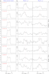 |
Fig. A.1. Observed lines of HC5N with the Yebes 40 m and IRAM 30 m telescopes. The rotational quantum numbers are indicated in the top-right side of each panel. The same transitions for the ν11 state are shown in the middle (e component) and right panels (f component). The intensity scale is antenna temperature in mK. The abscissa corresponds to LSR velocities in km s−1. The vertical red dotted line at −26.5 km s−1 indicates the systemic velocity of the envelope (Cernicharo et al. 2000, 2018). |
From the observed intensities of HC5N and its ν11 state, we performed a rotational diagram analysis. The results are shown in Fig. A.2. For the ground state, two different slopes, corresponding to two different rotational temperatures, were found. For low-J transitions in the Q-band, we derived Trot = 10.1 ± 0.6 K and N(HC5N) = 4.2 ± 0.4 × 1014 cm−2. The high-J data at 3 mm indicate a higher rotational temperature of 24.5 ± 0.6 K and a column density of 4.1 ± 0.3 × 1014 cm−2. The lines of the ν11 state are detected in the Q-band and the 3 mm domain and also show two different regimes: a low temperature component Trot = 13.0 ± 5.7 K and N(HC5N ν11) = 3.3 ± 1.8 × 1012 cm−2; and a high temperature component with Trot = 46.2 ± 13.8 K and N(HC5N ν11) = 4.4 ± 2.0 × 1012 cm−2. The observed column density ratio between the ground and the ν11 states is 127 ± 60 and 93 ± 50 for the cold and warm components, respectively. Consequently, the correction to the total column density of HC5N due to its vibrational state ν11 is ≃1%, that is to say the ground state contains more than 99% of the molecules. The observed column density ratio suggests a vibrational temperature ≃30 K, similar to the rotational temperature of the warm component.
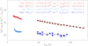 |
Fig. A.2. Rotational diagram for HC5N in its ground state (red) and ν11 = 1 vibrationally excited state (blue). |
A.2. HC7N
The rotational spectrum of HC7N in vibrationally excited states was recorded in the laboratory for ν13, ν14, and ν15 = 1, 2, 3 (Bizzocchi & Degli 2004). In this work, we detected all the lines of the ν15 = 1 state and some of the ν15 = 2 state within the covered 31–50 GHz frequency range. These two states lie at energies of ≈62 and 124 cm−1, respectively, above the ground state (Botschwina et al. 1997; Vichietti & Haiduke 2012). In the 70–116 GHz frequency range, only a few lines of the ν15 state are detected. Table A.3 gives the line parameters for the observed transitions of HC7N in its ground and vibrationally excited states, ν15 = 1 and ν15 = 2. Figure A.3 shows a selected sample of the observed lines. We have searched without success for lines arising from the ν14, and ν13 vibrational states within the covered frequency ranges. These states lie at energies of ≈163 and 280 cm−1, respectively, above the ground state (Botschwina et al. 1997; Vichietti & Haiduke 2012).
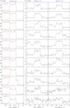 |
Fig. A.3. Observed lines of HC7N with the Yebes 40 m telescope. The rotational quantum numbers are indicated in the top-left side of each panel. The same transitions for the ν15 state are shown in the middle (e component) and right panels (f component). The intensity scale is antenna temperature in mK. The abscissa corresponds to LSR velocities in km s−1. The vertical red dotted line at −26.5 km s−1 indicates the systemic velocity of the envelope (Cernicharo et al. 2000, 2018). |
Same as Table A.2 but for HC7N.
Same as Table A.2 but for HC5N.
From the observed intensities of HC7N and its ν15 state, we performed a rotational diagram analysis. The results are shown in Fig. A.4. For the ground state, two different slopes, corresponding to two different rotational temperatures, were found; that is to say, the molecule shows a similar behavior to that of HC5N. For low-J transitions in the Q-band, we derived Trot = 16.8 ± 0.9 K and N(HC7N) = 1.9 ± 0.2 × 1014 cm−2. The high-J data at 3 mm indicate a higher rotational temperature of 32.6 ± 2.2 K and a column density of 8.4 ± 0.3 × 1013 cm−2. The lines of the ν15 state are mainly detected in the Q-band, for which we derive Trot = 21.6 ± 3.1 K and N(HC7N ν15) = 2.0 ± 0.5 × 1013 cm−2. Only a few rotational lines within the ν15 vibrational state were detected in the 3 mm domain and they are too weak to derive a reasonable rotational temperature and column density. For the Q-band data, which cover lines from Jup = 28 up to Jup = 44, the observed column density ratio between the ground and ν15 states is 9.5 ± 3.4. Consequently, the correction to the total column density of HC7N due to its vibrational state ν15 is ≃10%. Although the effect in the total column density is negligible, the observed column density in the ν15 level is a factor of ∼3 higher that the one we would expect if the vibrational levels were under thermodynamic equilibrium at the derived Trot. The observed column density ratio suggests a vibrational temperature of ≃30 K. As discussed in this letter, the increase in the population of the ν15 level is due to IR pumping from the ground state by absorption of IR photons coming from the central source and the subsequent IR radiative decay cascades. From the observed intensities of the ν15 = 2 lines, we derive a column density ratio of N(ν15 = 1)/N(ν15 = 2)≃5, which is also compatible with a vibrational temperature of 30 K. It is worth noting that this vibrational temperature is similar to the rotational temperature of the high-J lines of HC7N observed in the 3 mm domain, 26.2 ± 4.2 K. The effect of IR pumping on the ground state is, hence, to pump molecules from low-J levels to high-J ones.
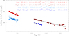 |
Fig. A.4. Rotational diagram for HC7N in its ground state (red) and ν15 = 1 vibrationally excited state (blue). |
Appendix B: Quantum chemical calculations for HC9N vibrationally excited states
We carried out quantum chemical calculations to obtain accurate values of the spectroscopic parameters necessary to assign the new spectral features. These parameters are the rotational constant B and the l-type doubling constant qe. To obtain these parameters for the vibrationally excited states of HC9N, we performed anharmonic frequency calculations. We used two different levels of theory for this purpose: density functional theory (DFT) calculations with the B3LYP functional (Lee et al. 1988) and the Møller–Plesset post-Hartree–Fock method (Møller & Plesset 1934), using explicitly electron correlation effects through perturbation theory up to second order (MP2). The Dunning basis set with consistent polarized valence triple-ζ (cc-pVTZ) was used in both calculation methods. The use of coupled cluster methods was not considered because of their large computing time. All the calculations were performed using the Gaussian 09 program package (Frisch et al. 2009). A previous theoretical study on the vibrationally excited states of HC9N, including other cyanopolyynes, was published by Vichietti & Haiduke (2012). However, the authors only provide the vibrational band frequencies and intensities under the harmonic approximation. The results of our anharmonic calculations in terms of energy and intensities are compatible with those reported by Vichietti & Haiduke (2012).
The value of Bν for each vibrationally excited state of HC9N can be determined using the values of the first order vibration-rotation coupling constants αi, which are different for each vibrational state and are obtained from the anharmonic frequency calculations. Values of Bν can be derived using the expression (Gordy & Cook 1984)
 (B.1)
(B.1)
where Bν and Be are the rotational constant in a given excited state and in equilibrium, respectively, νi is the vibrational quantum number, and di is the corresponding degeneracy of the state. On the other hand, the values for the l-type doubling constant  can be directly obtained from the frequency calculations.
Table B.1 shows the vibration-rotation coupling constants αi and the l-type doubling constant  for each vibrationally excited state i of HC9N obtained from the B3LYP and MP2 calculations. The estimated rotational constants for each vibrationally excited state were calculated as described above using the Bground constant for the ground state determined by Iida et al. (1991). The anharmonic vibrational frequencies and the IR intensities of the corresponding fundamental bands are also shown in Table B.1. The assignment of the observed transitions to the vibrationally excited state ν19 = 1 is based on the excellent agreement between the experimental and predicted values for B19 and the
  . It can be observed that the accordance between the experimental and predicted values is a bit better when the B3LYP/cc-pVTZ level of theory is used. However, the theoretical results for both methods indicate that the assignment is unequivocal regardless of the level of the calculation. Further evidence in support of this assignment is related to the vibrational frequency. Using the experimental values derived from the rotational analysis and the approximate expression
  (Gordy & Cook 1984), the obtained value for the vibrational frequency is only compatible with the assignment of the series of lines to the ν19 state.
Theoretical values for the vibrational excited states of HC9N calculated at B3LYP/cc-pVTZ and MP2/cc-pVTZ levels of theory under the anharmonic approach.
The reliability of both methods of calculation used for HC9N was first tested for the analogue molecular systems HC5N and HC7N to rule out any kind of doubt in the assignment. Tables B.2 and B.3 show the results of anharmonic calculations for HC5N and HC7N at both B3LYP/cc-pVTZ and MP2/cc-pVTZ levels of theory. The values of Bν and  calculated for HC5N and HC7N are compared to those reported experimentally (Bizzocchi & Degli 2004; Yamada et al. 2004; Degli Esposti et al. 2005). We see that the predicted values with both levels of theory reproduce the experimental values for the two molecules very well. The errors obtained for HC5N and HC7N are on the same order of those found for the ν19 mode of HC9N. As is usually observed for linear molecules, the values of
  obtained by these calculations are slightly lower than the corresponding experimental values. Finally, Table B.4 collects the energies and intensities of the fundamental bands of all the vibrational modes of HC5N, HC7N, and HC9N calculated at the MP2 and B3LYP levels of theory.
Comparison between experimental and theoretical values, using the anharmonic approximation at B3LYP/cc-pVTZ level of theory, for the vibrationally excited states of HC5N and HC7N.
Comparison between experimental and theoretical values, using the anharmonic approximation at MP2/cc-pVTZ level of theory, for the vibrationally excited states of HC5N and HC7N.
Calculated energies and IR intensities of the fundamental bands of all the vibrational modes of HC5N, HC7N, and HC9N.
All Tables
Theoretical values for the vibrational excited states of HC9N calculated at B3LYP/cc-pVTZ and MP2/cc-pVTZ levels of theory under the anharmonic approach.
Comparison between experimental and theoretical values, using the anharmonic approximation at B3LYP/cc-pVTZ level of theory, for the vibrationally excited states of HC5N and HC7N.
Comparison between experimental and theoretical values, using the anharmonic approximation at MP2/cc-pVTZ level of theory, for the vibrationally excited states of HC5N and HC7N.
Calculated energies and IR intensities of the fundamental bands of all the vibrational modes of HC5N, HC7N, and HC9N.
All Figures
|
Fig. 1. Data from two frequency ranges within the Q-band observed with the Yebes 40 m telescope towards IRC +10216. Each frequency range is shown through two panels with different limits in intensity. The vertical scale is antenna temperature in mK. The horizontal scale is the rest frequency in MHz. Labels for HC7N features are in blue, while those belonging to HC9N are in violet. Other spectral features from known species, together with unidentified lines (labeled as “U” lines), are indicated in red. The N = 16−15 doublet of MgCCCN, a new species recently detected (Cernicharo et al. 2019), is shown in the bottom panels. Vibrationally excited lines from HC7N, HC9N, and C6H are nicely detected at these frequencies. Additional lines from vibrationally excited states of HC5N, HC7N, and HC9N are shown in Figs. 2, A.1, and A.3. |
| In the text | |
|
Fig. 2. Selected doublets of HC9N ν19 = 1 in the 31–50 GHz domain. Left panels: lines of HC9N in the ground vibrational state. The rotational quantum numbers are indicated in the top-right side of each panel. The same transitions for the ν19 = 1 state are shown in the middle (e component) and right (f component) panels. The intensity scale is antenna temperature in mK. The abscissa corresponds to local standard of rest (LSR) velocities in km s−1. The vertical violet dotted line at −26.5 km s−1 indicates the systemic velocity of the envelope (Cernicharo et al. 2000, 2018). Two additional ν19 doublets are shown in Fig. 1. |
| In the text | |
|
Fig. 3. Rotational diagram of HC9N in its ground state (red) and ν19 = 1 vibrationally excited state (blue). The derived rotational temperatures and column densities are indicated in the plot. |
| In the text | |
|
Fig. 4. Calculated line profiles for selected lines of HC5N, HC7N, and HC9N in their ground state (G.S.) and lowest energy bending vibrational states. Calculated intensities have been multiplied by 10, 8, and 2 for HC5N, HC7N, and HC9N, respectively, to match the observed intensities of the ground vibrational state lines. |
| In the text | |
|
Fig. A.1. Observed lines of HC5N with the Yebes 40 m and IRAM 30 m telescopes. The rotational quantum numbers are indicated in the top-right side of each panel. The same transitions for the ν11 state are shown in the middle (e component) and right panels (f component). The intensity scale is antenna temperature in mK. The abscissa corresponds to LSR velocities in km s−1. The vertical red dotted line at −26.5 km s−1 indicates the systemic velocity of the envelope (Cernicharo et al. 2000, 2018). |
| In the text | |
|
Fig. A.2. Rotational diagram for HC5N in its ground state (red) and ν11 = 1 vibrationally excited state (blue). |
| In the text | |
|
Fig. A.3. Observed lines of HC7N with the Yebes 40 m telescope. The rotational quantum numbers are indicated in the top-left side of each panel. The same transitions for the ν15 state are shown in the middle (e component) and right panels (f component). The intensity scale is antenna temperature in mK. The abscissa corresponds to LSR velocities in km s−1. The vertical red dotted line at −26.5 km s−1 indicates the systemic velocity of the envelope (Cernicharo et al. 2000, 2018). |
| In the text | |
|
Fig. A.4. Rotational diagram for HC7N in its ground state (red) and ν15 = 1 vibrationally excited state (blue). |
| In the text | |
Current usage metrics show cumulative count of Article Views (full-text article views including HTML views, PDF and ePub downloads, according to the available data) and Abstracts Views on Vision4Press platform.
Data correspond to usage on the plateform after 2015. The current usage metrics is available 48-96 hours after online publication and is updated daily on week days.
Initial download of the metrics may take a while.