© ESO 2020

1. Introduction

One important goal of extragalactic astronomy and cosmology is understanding galaxy formation and evolution. The following two different types of simulations try to reproduce the observed galaxy and matter distribution: full hydrodynamical simulations (e.g. Vogelsberger et al. 2014; Crain et al. 2015; Kaviraj et al. 2017; Nelson et al. 2019) and dark-matter-only N-body simulations with galaxies inserted according to semi-analytic models (SAMs) of galaxy formation and evolution.

Multiple SAMs, with different assumptions on small-scale physics, such as the gas cooling time, the star formation rate, or supernovae feedback, have been proposed (e.g. Bower et al. 2006; Guo et al. 2011; Lagos et al. 2012; Henriques et al. 2015). These models must be assessed by comparing their predictions to observations of galaxy statistics. Previous tests of SAMs included galaxy-galaxy lensing (GGL; e.g. Saghiha et al. 2017) and galaxy clustering (e.g. Henriques et al. 2017).

A more sensitive test than GGL is comparing the galaxy–galaxy–galaxy lensing (G3L) signal predicted by the SAMs to observations. The G3L effect, which was first discussed by Schneider & Watts (2005), describes the weak gravitational lensing of pairs of background galaxies around foreground galaxies (lens-shear-shear correlation) and of individual background galaxies around pairs of foreground galaxies (lens-lens-shear correlation). Unlike GGL or galaxy clustering, G3L depends on the galaxy-matter three-point correlation and the halo occupation distribution of galaxy pairs. In principle, it also depends on the ellipticity of dark matter halos as well as misalignments between the galaxy and matter distribution because the galaxy pair orientation introduces a preferred direction.

The lens-lens-shear correlation was measured for lens pairs separated by several megaparsecs (Mpc) in order to detect inter-cluster filaments (Mead et al. 2010; Clampitt et al. 2016; Epps & Hudson 2017; Xia et al. 2020). However, for the evaluation of SAMs, it is more suitable to study the correlation at smaller, sub-Mpc scales. At these scales, the G3L signal is more sensitive to the small-scale physics that vary between different SAMs, because it depends primarily on galaxy pairs with galaxies in the same dark matter halo. For lens pairs with galaxies of a similar stellar mass or colour, the small-scale lens-lens-shear correlation was determined by Simon et al. (2008) in the Red Cluster Sequence survey (Hildebrandt et al. 2016) and Simon et al. (2013) in the Canada-France-Hawaii Telescope Lensing Survey (CFHTLenS; Heymans et al. 2012). The G3L measured in CFHTLenS was compared to predictions by multiple SAMs that were implemented in the Millennium Run (MR; Springel et al. 2005) by Saghiha et al. (2017) and Simon et al. (2019). They demonstrate that G3L is more effective in evaluating SAMs than GGL and that the SAM by Henriques et al. (2015, H15 hereafter) is in agreement with the observations in CFHTLenS, while the SAM by Lagos et al. (2012, L12 hereafter) predicts G3L signals that are too large.

Nonetheless, these previous measurements of G3L at small scales only used photometric data with imprecise redshift estimates for the lens galaxies. Therefore, lens galaxy pairs with galaxies separated along the line-of-sight (chance pairs) were treated the same as lens galaxy pairs with galaxies close to each other (true pairs). As the G3L signal of chance pairs is much weaker, this lowers the signal-to-noise ratio (S/N).

However, Linke et al. (2020, L20 hereafter) demonstrate that the S/N could be improved substantially by weighting each lens galaxy pair according to the line-of-sight separation between its galaxies to reduce the impact of chance pairs. We used this improved estimator to test the H15 and the L12 SAMs with state-of-the-art observational data, consisting of the photometric Kilo-Degree Survey (KiDS) and VISTA Kilo-degree Infrared Galaxy survey (VIKING) as well as the spectroscopic Galaxy And Mass Assembly survey (GAMA). We used the shapes of galaxies observed by KiDS as shear estimates, while GAMA provides lens galaxies with precise spectroscopic redshifts. These spectroscopic redshifts allowed us to employ the redshift weighting suggested by L20. Furthermore, we extended the angular range at which we measured the G3L signal to lower scales with the adaptive binning scheme for the G3L three-point correlation function proposed by L20. Thereby, we could assess the SAMs deeper inside dark-matter halos.

As of now, the lens-lens-shear correlation has only been measured for lens pairs with galaxies from the same colour or stellar-mass sample (unmixed lens pairs) and not for lens pairs with galaxies from different samples (mixed lens pairs). However, comparing the measurements for G3L with mixed pairs is a compelling new test of SAMs, because this signal depends on the correlation of different galaxy populations inside halos. For example, the mixed pair G3L signal would be higher for two fully correlated galaxy populations than for two uncorrelated populations, while the GGL signal would stay the same. Therefore, we can assess the predictions of SAMs for the correlation between different galaxy populations with the G3L of mixed lens pairs. Accordingly, we measure not only the G3L signal for lens pairs from the same population but also the signal for mixed lens pairs, with galaxies from different colour- or stellar-mass samples.

This paper is structured as follows: in Sect. 2 we review the basics of G3L and introduce the third-order aperture statistics, which are the G3L observables throughout this work. Section 3 discusses our estimators for the three-point correlation function and the aperture statistics. The SAMs and the creation of the simulated and observational data sets are described in Sect. 4. We present the G3L signals measured in the observation and the simulation in Sect. 5 and discuss our findings in Sect. 6.

Throughout this paper we assume a flat ΛCDM cosmology with matter density Ω_m = 0.25, baryon density Ω_b = 0.045, dark energy density Ω_Λ = 0.75, Hubble constant H₀ = 73 km s⁻¹ Mpc⁻¹ and power spectrum normalisation σ₈ = 0.9. These parameters were used in the creation of the MR and differ from more recent constraints (e.g. Planck Collaboration I 2020). However, weak gravitational lensing is most sensitive to the combination of the matter density and the power spectrum normalisation $S_8={\sigma }_8\sqrt{{\mathrm{\Omega }}_{\text{m}}/0.3}$. This parameter is almost the same in the MR and the most recent Planck measurements; it is S_8, MR = 0.822 for the MR and S_8, Planck = 0.825 ± 0.011 in Planck Collaboration I (2020).

2. Theory of galaxy–galaxy–galaxy lensing

G3L is a weak gravitational lensing effect (see e.g. Bartelmann & Schneider 2001). It comprises the correlation of individual lens galaxies with the shear of source galaxy pairs, as well as the correlation of lens galaxy pairs with the shear of individual source galaxies. Here, we study the second effect, the lens-lens-shear correlation. Figure 1 illustrates the geometric configuration of lens and source galaxies for this correlation.

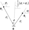Fig. 1. Geometry of a G3L configuration with one source and two lens galaxies; adapted from Schneider & Watts (2005). The two lens galaxies are at angular positions θ1 and θ2 on the sky; the source galaxy is at θ. The separation vectors ϑ1 and ϑ2 of the lenses from the source have lengths ϑ1 and ϑ2, as well as polar angles φ1 and φ2. The angle between ϑ1 and ϑ2 is the opening angle ϕ. The tangential shear of the source galaxy is measured with respect to the dashed line, which is the bisector of ϕ.

2.1. Three-point correlation function

The main observable for the lens-lens-shear correlation is the three-point correlation function $\stackrel{\sim }{\mathcal{G}}$. This function correlates the projected lens galaxy number density and the tangential gravitational lensing shear γ_t, measured with respect to the bisector of the angle ϕ between the lens-source separations ϑ₁ and ϑ₂ (see Fig. 1). For unmixed lens pairs, whose galaxies have the projected number density N(ϑ), $\stackrel{\sim }{\mathcal{G}}$ is

$$\begin{array}{c}\hfill \stackrel{\sim }{\mathcal{G}}({\mathit{\vartheta }}_{\mathbf{1}},{\mathit{\vartheta }}_{\mathbf{2}})={\displaystyle \frac{1}{{\overline{N}}^2}}⟨N(\mathit{\theta }+{\mathit{\vartheta }}_{\mathbf{1}})N(\mathit{\theta }+{\mathit{\vartheta }}_{\mathbf{2}}){\gamma }_{\text{t}}(\mathit{\theta })⟩,\end{array}$$(1)

where $\overline{N}$ is the mean number density of lenses. For mixed lens pairs, where the lenses are from samples with number densities N₁ and N₂, the correlation function is

$$\begin{array}{c}\hfill \stackrel{\sim }{\mathcal{G}}({\mathit{\vartheta }}_{\mathbf{1}},{\mathit{\vartheta }}_{\mathbf{2}})=\frac{1}{{\overline{N}}_1{\overline{N}}_2}⟨N_1(\mathit{\theta }+{\mathit{\vartheta }}_1)N_2(\mathit{\theta }+{\mathit{\vartheta }}_{\mathbf{2}}){\gamma }_{\text{t}}(\mathit{\theta })⟩.\end{array}$$(2)

Instead of measuring $\stackrel{\sim }{\mathcal{G}}$, we estimated a redshift-weighted correlation function ${\stackrel{\sim }{\mathcal{G}}}_Z$, which includes a redshift weighting function Z, which depends on the redshift difference Δz₁₂ = z₁ − z₂ of the lenses in a pair. We chose the redshift weighting such that it is large for small Δz₁₂ and vanishes for large Δz₁₂. It, therefore, weights true pairs with small redshift differences higher than chance pairs with large redshift differences and increases the S/N (L20). To define the redshift-weighted correlation function ${\stackrel{\sim }{\mathcal{G}}}_Z$, we used that the projected lens number densities N_1, 2 are related to the three-dimensional number densities n_1, 2(θ, z) at redshift z by the selection functions ν_1, 2(z),

$$\begin{array}{c}\hfill N_{1,2}(\mathit{\theta })={\displaystyle \int \mathrm{d}z}{\nu }_{1,2}(z)n_{1,2}(\mathit{\theta },z).\end{array}$$(3)

The selection functions give the fraction of galaxies at redshift z included in the lens sample. For a flux-limited galaxy sample, this corresponds to the fraction of galaxies brighter than the magnitude limit. The selection functions ν_1, 2(z) are related to the galaxies’ redshift distributions p_1, 2(z) by

$$\begin{array}{c}\hfill {\nu }_{1,2}(z)=p_{1,2}(z)\frac{{\int }_A{\mathrm{d}}^2\theta N_{1,2}(\mathit{\theta })}{{\int }_A{\mathrm{d}}^2\theta n_{1,2}(\mathit{\theta },z)}\end{array}$$(4)

with Eq. (3), the redshift-weighted correlation function is

$$\begin{array}{cc}& {\stackrel{\sim }{\mathcal{G}}}_Z({\mathit{\vartheta }}_{\mathbf{1}},{\mathit{\vartheta }}_{\mathbf{2}})\hfill \\ \hfill & ={\left[{\displaystyle {\int }_0^{\infty }}\mathrm{d}{z}_1{\displaystyle {\int }_0^{\infty }}\mathrm{d}{z}_2{\nu }_1(z_1){\nu }_2(z_2)Z(\mathrm{\Delta }{z}_{12}){\overline{n}}_1(z_1){\overline{n}}_2(z_2)\right]}^{-1}\hfill \\ \hfill & \times {\displaystyle {\int }_0^{\infty }}\mathrm{d}{z}_1{\displaystyle {\int }_0^{\infty }}\mathrm{d}{z}_2{\nu }_1(z_1){\nu }_2(z_2)Z(\mathrm{\Delta }{z}_{12})\hfill \\ \hfill & \times ⟨n_1(\mathit{\theta }+{\mathit{\vartheta }}_{\mathbf{1}},z_1)n_2(\mathit{\theta }+{\mathit{\vartheta }}_{\mathbf{2}},z_2){\gamma }_{\text{t}}(\mathit{\theta })⟩,\hfill \end{array}$$(5)

where Δz₁₂ := z₁ − z₂ is the redshift difference between lenses in a pair and

$$\begin{array}{c}\hfill {\overline{n}}_{1,2}(z)=⟨n_{1,2}(\mathit{\theta }\mathbf{,}\mathit{z})⟩=\frac{1}{A}{\displaystyle {\int }_A}{\mathrm{d}}^2\theta n_{1,2}(\mathit{\theta },z).\end{array}$$(6)

Additionally, we also measured the physical correlation function ${\stackrel{\sim }{\mathcal{G}}}_{\text{phys}}({\mathit{r}}_{\mathbf{1}},{\mathit{r}}_{\mathbf{2}})$, which gives the projected excess mass around lens pairs with physical lens-source separations r₁ and r₂ projected on a plane midway between the lenses. To find ${\stackrel{\sim }{\mathcal{G}}}_{\text{phys}}$, instead of averaging the tangential shear γ_t, we averaged the projected excess mass density ΔΣ around lens pairs with

$$\begin{array}{cc}& {\stackrel{\sim }{\mathcal{G}}}_{\text{phys}}({\mathit{r}}_{\mathbf{1}},{\mathit{r}}_{\mathbf{2}})\hfill \\ \hfill & ={\left[{\displaystyle {\int }_0^{\infty }}\mathrm{d}{z}_1{\displaystyle {\int }_0^{\infty }}\mathrm{d}{z}_2{\nu }_1(z_1){\nu }_2(z_2)Z(\mathrm{\Delta }{z}_{12}){\overline{n}}_1(z_1){\overline{n}}_2(z_2)\right]}^{-1}\hfill \\ \hfill & \times {\displaystyle \int \mathrm{d}{z}_1\int \mathrm{d}{z}_2}{\nu }_1(z_1){\nu }_2(z_2)Z(\mathrm{\Delta }{z}_{12})\hfill \\ \hfill & \times ⟨n_1(\mathit{\theta }+D_{12}^{-1}{\mathit{r}}_{\mathbf{1}},z_1)n_2(\mathit{\theta }+D_{12}^{-1}{\mathit{r}}_{\mathbf{2}},z_2)\mathrm{\Delta }\mathrm{\Sigma }(\mathit{\theta },z_{12})⟩,\hfill \end{array}$$(7)

where

$$\begin{array}{c}\hfill z_{12}=\frac{z_1+z_2}{2},\end{array}$$(8)

and

$$\begin{array}{c}\hfill D_{12}=D_{\mathrm{A}}(0,z_{12}),\end{array}$$(9)

with the angular diameter distance D_A(z₁, z₂) between redshifts z₁ and z₂. The projected excess mass density ΔΣ is

$$\begin{array}{c}\hfill \mathrm{\Delta }\mathrm{\Sigma }(\mathit{\theta },z_{\text{d}})={\displaystyle \frac{{\gamma }_{\text{t}}(\mathit{\theta })}{{\overline{\mathrm{\Sigma }}}_{\text{crit}}^{-1}(z_{\text{d}})}},\end{array}$$(10)

with the source-averaged inverse critical surface mass density ${\overline{\mathrm{\Sigma }}}_{\mathrm{crit}}^{-1}$. Using the source redshift distribution p(z_s), ${\overline{\mathrm{\Sigma }}}_{\mathrm{crit}}^{-1}$ is

$$\begin{array}{c}\hfill {\overline{\mathrm{\Sigma }}}_{\text{crit}}^{-1}(z_{\text{d}})={\displaystyle {\int }_{z_{\text{d}}}^{\infty }}\mathrm{d}{z}_{\text{s}}p(z_{\text{s}})\frac{4\pi G}{c^2}\frac{D_{\text{A}}(z_{\text{d}},z_{\text{s}})D_{\text{A}}(z_{\text{d}})}{D_{\text{A}}(z_{\text{s}})},\end{array}$$(11)

where D_A(z) := D_A(0, z). This critical surface mass density is not the comoving critical surface mass density ${\overline{\mathrm{\Sigma }}}_{\text{crit, com}}$, defined by

$$\begin{array}{c}\hfill {\overline{\mathrm{\Sigma }}}_{\text{crit,com}}^{-1}(z_{\text{d}})={\displaystyle {\int }_{z_{\text{d}}}^{\infty }}\mathrm{d}{z}_{\text{s}}p(z_{\text{s}})\frac{4\pi G}{c^2}\frac{D_{\text{A}}(z_{\text{d}},z_{\text{s}})D_{\text{A}}(z_{\text{d}})}{(1+z_{\mathrm{d}})D_{\text{A}}(z_{\text{s}})},\end{array}$$

used in some weak lensing studies. Appendix C in Dvornik et al. (2018) discusses the implications of different definitions of the critical surface mass density.

The correlation functions ${\stackrel{\sim }{\mathcal{G}}}_Z$ and ${\stackrel{\sim }{\mathcal{G}}}_{\text{phys}}$ depend only on the lens-source distances ϑ₁, ϑ₂ and r₁, r₂, and the opening angle ϕ between the lens-source separations, because of the statistical isotropy of the matter and galaxy density fields. Therefore, we define

$$\begin{array}{c}\hfill {\stackrel{\sim }{\mathcal{G}}}_Z({\vartheta }_1,{\vartheta }_2,\varphi ):={\stackrel{\sim }{\mathcal{G}}}_Z({\mathit{\vartheta }}_{\mathbf{1}},{\mathit{\vartheta }}_{\mathbf{2}}),\end{array}$$(12)

and

$$\begin{array}{c}\hfill {\stackrel{\sim }{\mathcal{G}}}_{\text{phys}}(r_1,r_2,\varphi ):={\stackrel{\sim }{\mathcal{G}}}_{\text{phys}}({\mathit{r}}_{\mathbf{1}},{\mathit{r}}_{\mathbf{2}}).\end{array}$$(13)

2.2. Aperture statistics

The three-point correlation function $\stackrel{\sim }{\mathcal{G}}$ contains second- and third-order statistics. This can be seen by writing $\stackrel{\sim }{\mathcal{G}}$ as

$$\begin{array}{cc}\hfill \stackrel{\sim }{\mathcal{G}}({\vartheta }_1,{\vartheta }_2,\varphi )& =⟨{\kappa }_{\text{g}}(\mathit{\theta }+{\mathit{\vartheta }}_{\mathbf{1}}){\kappa }_{\text{g}}(\mathit{\theta }+{\mathit{\vartheta }}_{\mathbf{2}}){\gamma }_{\text{t}}(\mathit{\theta })⟩\hfill \\ \hfill & +⟨{\kappa }_{\text{g}}(\mathit{\theta }+{\mathit{\vartheta }}_{\mathbf{1}}){\gamma }_{\text{t}}(\mathit{\theta })⟩+⟨{\kappa }_{\text{g}}(\mathit{\theta }+{\mathit{\vartheta }}_{\mathbf{2}}){\gamma }_{\text{t}}(\mathit{\theta })⟩,\hfill \end{array}$$(14)

where ${\kappa }_{\text{g}}(\mathit{\vartheta })=N(\mathit{\vartheta })/\overline{N}-1$ is the two-dimensional galaxy number density contrast. The second and third term in Eq. (14) are GGL statistics which correspond to the shear around individual lens galaxies.

When studying G3L we are interested in the excess shear around lens pairs, which is given only by the first term in Eq. (14). Therefore, we converted ${\stackrel{\sim }{\mathcal{G}}}_Z$ and ${\stackrel{\sim }{\mathcal{G}}}_{\text{phys}}$ to the third-order aperture statistics ⟨𝒩𝒩M_ap⟩ and ⟨𝒩𝒩M_ap⟩_phys, which only include the third-order statistics, as shown in L20. For this, we use a compensated filter function with an aperture scale θ,

$$\begin{array}{c}\hfill U_{\theta }(\vartheta )=\frac{1}{{\theta }^2}u\left(\frac{\vartheta }{\theta }\right),\end{array}$$(15)

which fulfills

$$\begin{array}{c}\hfill {\displaystyle \int \mathrm{d}\vartheta }\vartheta U_{\theta }(\vartheta )=0\end{array}$$(16)

with this filter function, the third-order aperture statistics are defined as

$$\begin{array}{cc}& ⟨\mathcal{NN}{M}_{\mathrm{ap}}⟩({\theta }_1,{\theta }_2,{\theta }_3)\hfill \\ \hfill & ={\left[{\displaystyle {\int }_0^{\infty }}\mathrm{d}{z}_1{\displaystyle {\int }_0^{\infty }}\mathrm{d}{z}_{2}Z(\mathrm{\Delta }{z}_{12}){\overline{n}}_1(z_1){\overline{n}}_2(z_2)\right]}^{-1}\hfill \\ \hfill & \times {\displaystyle {\int }_0^{\infty }}\mathrm{d}{z}_1{\displaystyle {\int }_0^{\infty }}\mathrm{d}{z}_{2}Z(\mathrm{\Delta }{z}_{12})\left[{\displaystyle \prod _{i=1}^3\int {\mathrm{d}}^2}{\vartheta }_i\frac{1}{{\theta }_i^2}u\left(\frac{{\vartheta }_i}{{\theta }_i}\right)\right]\hfill \\ \hfill & \times ⟨n_1({\mathit{\vartheta }}_{\mathbf{1}},z_1)n_2({\mathit{\vartheta }}_{\mathbf{2}},z_2)\kappa ({\mathit{\vartheta }}_{\mathbf{3}})⟩,\hfill \end{array}$$(17)

and

$$\begin{array}{cc}& {⟨\mathcal{NN}{M}_{\mathrm{ap}}⟩}_{\text{phys}}(r_1,r_2,r_3)\hfill \\ \hfill & ={\left[{\displaystyle {\int }_0^{\infty }}\mathrm{d}{z}_1{\displaystyle {\int }_0^{\infty }}\mathrm{d}{z}_{2}Z(\mathrm{\Delta }{z}_{12}){\overline{n}}_1(z_1){\overline{n}}_2(z_2)\right]}^{-1}\hfill \\ \hfill & \times {\displaystyle {\int }_0^{\infty }}\mathrm{d}{z}_1{\displaystyle {\int }_0^{\infty }}\mathrm{d}{z}_{2}Z(\mathrm{\Delta }{z}_{12})\left[{\displaystyle \prod _{i=1}^3\int {\mathrm{d}}^2}{x}_i\frac{1}{D_{12}^{-2}{r}_i^2}u\left(\frac{x_i}{r_i}\right)\right]\hfill \\ \hfill & \times ⟨n_1(D_{12}^{-1}{\mathit{x}}_{\mathbf{1}},z_1)n_2(D_{12}^{-1}{\mathit{x}}_{\mathbf{2}},z_2)\mathrm{\Sigma }(D_{12}^{-1}{\mathit{x}}_{\mathbf{3}},z_{12}⟩,\hfill \end{array}$$(18)

with the lensing convergence κ(θ) and the surface mass density Σ, given by

$$\begin{array}{c}\hfill \mathrm{\Sigma }(\mathit{\theta },z)=\frac{\kappa (\mathit{\theta })}{{\overline{\mathrm{\Sigma }}}_{\text{crit}}^{-1}(z)}·\end{array}$$(19)

We use the exponential filter function

$$\begin{array}{c}\hfill u(x)=\frac{1}{2\pi }(1-\frac{x^2}{2})exp(-\frac{x^2}{2}),\end{array}$$(20)

for which the aperture statistics can be calculated from ${\stackrel{\sim }{\mathcal{G}}}_Z$ and ${\stackrel{\sim }{\mathcal{G}}}_{\text{phys}}$ with

$$\begin{array}{cc}& ⟨\mathcal{NN}{M}_{\mathrm{ap}}⟩({\theta }_1,{\theta }_2,{\theta }_3)\hfill \\ \hfill & ={\displaystyle {\int }_0^{\infty }}\mathrm{d}{\vartheta }_1{\vartheta }_1{\displaystyle {\int }_0^{\infty }}\mathrm{d}{\vartheta }_2{\vartheta }_2{\displaystyle {\int }_0^{2\pi }}\mathrm{d}\varphi {\stackrel{\sim }{\mathcal{G}}}_Z({\vartheta }_1,{\vartheta }_2,\varphi )\hfill \\ \hfill & \times {\mathcal{A}}_{\mathcal{N}\mathcal{N}\mathcal{M}}({\vartheta }_1,{\vartheta }_2,\varphi |{\theta }_1,{\theta }_2,{\theta }_3).\hfill \end{array}$$(21)

and

$$\begin{array}{cc}& {⟨\mathcal{NN}{M}_{\mathrm{ap}}⟩}_{\text{phys}}(r_1,r_2,r_3)\hfill \\ \hfill & ={\displaystyle {\int }_0^{\infty }}\mathrm{d}{x}_1{x}_1{\displaystyle {\int }_0^{\infty }}\mathrm{d}{x}_2{x}_2{\displaystyle {\int }_0^{2\pi }}\mathrm{d}\varphi {\stackrel{\sim }{\mathcal{G}}}_{\text{phys}}(x_1,x_2,\varphi )\hfill \\ \hfill & \times {\mathcal{A}}_{\mathcal{N}\mathcal{N}\mathcal{M}}(x_1,x_2,\varphi |r_1,r_2,r_3).\hfill \end{array}$$(22)

The kernel function 𝒜_𝒩𝒩ℳ is defined in the appendix of Schneider & Watts (2005).

2.3. Galaxy bias

The aperture statistics can be used to constrain the galaxy bias, which is the relation between the galaxy number density contrast and the matter density contrast (e.g Schneider & Watts 2005). The simplest assumption for this bias is a linear deterministic relation,

$$\begin{array}{c}\hfill {\kappa }_{\text{g}}(\mathit{\theta })=b\kappa (\mathit{\theta }),\end{array}$$(23)

where b is a scale-independent bias factor (Kaiser 1984). A larger bias factor b implies a higher galaxy number density for a given matter overdensity. For two galaxy populations with bias factors b₁ and b₂, this simple model predicts for the aperture statistics

$$\begin{array}{c}\hfill ⟨{\mathcal{N}}_1{\mathcal{N}}_2{M}_{\text{ap}}⟩\propto b_1{b}_2.\end{array}$$(24)

From this follows, that

$$\begin{array}{c}\hfill R:=\frac{⟨{\mathcal{N}}_1{\mathcal{N}}_2{M}_{\text{ap}}⟩}{\sqrt{⟨{\mathcal{N}}_1{\mathcal{N}}_1{M}_{\text{ap}}⟩⟨{\mathcal{N}}_2{\mathcal{N}}_2{M}_{\text{ap}}⟩}}=\frac{b_1{b}_2}{\sqrt{b_1^2{b}_2^2}}=1.\end{array}$$(25)

We measure R in the observation and simulation to assess the assumption of linear deterministic bias.

3. Methods

3.1. Estimating the three-point correlation function

To measure ${\stackrel{\sim }{\mathcal{G}}}_Z$ and ${\stackrel{\sim }{\mathcal{G}}}_{\text{phys}}$, we used the estimators from L20 for N_s source and N_d lens galaxies. These estimators measure the correlation functions by averaging the ellipticities of the source galaxies over all lens-lens-source galaxy triplets. For ${\stackrel{\sim }{\mathcal{G}}}_Z$, in the bin B of (ϑ₁, ϑ₂, ϕ), the estimator is the real part of

$$\begin{array}{cc}& {\stackrel{\sim }{\mathcal{G}}}_{Z,\text{est}}(B)\hfill \\ \hfill & =-\frac{{\displaystyle \sum _{i,j=1}^{N_{\text{d}}}\sum _{k=1}^{N_{\text{s}}}}{w}_k{ϵ}_k{\text{e}}^{-\text{i}({\phi }_{\mathit{ik}}+{\phi }_{\mathit{jk}})}[1+{\omega }_Z(|{\mathit{\theta }}_{\mathit{i}}-{\mathit{\theta }}_{\mathit{j}}|)]Z(\mathrm{\Delta }{z}_{\mathit{ij}}){\mathrm{\Delta }}_{\mathit{ijk}}(B)}{{\displaystyle \sum _{i,j=1}^{N_{\text{d}}}\sum _{k=1}^{N_{\text{s}}}}{w}_{k}Z(\mathrm{\Delta }{z}_{\mathit{ij}}){\mathrm{\Delta }}_{\mathit{ijk}}(B)}\hfill \end{array}$$(26)

$$\begin{array}{cc}& :=-{\displaystyle \frac{{\displaystyle \sum _{\mathit{ijk}}}{w}_k{ϵ}_k{\text{e}}^{-\text{i}({\phi }_{\mathit{ik}}+{\phi }_{\mathit{jk}})}[1+{\omega }_Z(|{\mathit{\theta }}_{\mathit{i}}-{\mathit{\theta }}_{\mathit{j}}|)]Z(\mathrm{\Delta }{z}_{\mathit{ij}}){\mathrm{\Delta }}_{\mathit{ijk}}(B)}{{\displaystyle \sum _{\mathit{ijk}}}{w}_{k}Z(\mathrm{\Delta }{z}_{\mathit{ij}}){\mathrm{\Delta }}_{\mathit{ijk}}(B)}},\hfill \end{array}$$(27)

where w_k is the weight of the source ellipticity ϵ_k, ω_Z is the redshift-weighted angular two-point correlation function of the lens galaxies, and

$$\begin{array}{c}\hfill {\mathrm{\Delta }}_{\mathit{ijk}}(B)=\{\begin{array}{cc}1\hfill & \text{for}(|{\mathit{\theta }}_{\mathit{k}}-{\mathit{\theta }}_{\mathit{i}}|,|{\mathit{\theta }}_{\mathit{k}}-{\mathit{\theta }}_{\mathit{j}}|,{\varphi }_{\mathit{ijk}})\in B\hfill \\ 0\hfill & \text{otherwise}\hfill \end{array}.\end{array}$$(28)

The angles φ_ik and φ_jk are the polar angles of the lens-source separation vectors θ_i − θ_k and θ_j − θ_k (corresponding to φ₁ and φ₂ in Fig. 1) and ϕ_ijk = φ_ik − φ_jk is the opening angle between the lens-source separation vectors (corresponding to ϕ in Fig. 1).

Source galaxies with more precise shape measurements receive a higher ellipticity weight w_k. The weight, therefore, increases the contribution of source galaxies with more exact shapes to the estimator. For the simulated shear data, we set the weights to w_k = 1 for all sources.

We obtained the lens two-point correlation function ω_Z, with the estimator by Szapudi & Szalay (1998) which is

$$\begin{array}{c}\hfill {\omega }_Z(\theta )=\frac{N_{{\text{r}}_1}{N}_{{\text{r}}_2}}{N_{{\text{d}}_1}{N}_{{\text{d}}_2}}\frac{{D_1{D}_2}_Z(\theta )}{{R_1{R}_2}_Z(\theta )}-\frac{N_{{\text{r}}_1}}{N_{{\text{d}}_1}}\frac{{D_1{R}_2}_Z(\theta )}{{R_1{R}_2}_Z(\theta )}-\frac{N_{{\text{r}}_2}}{N_{{\text{d}}_2}}\frac{{D_2{R}_1}_Z(\theta )}{{R_1{R}_2}_Z(\theta )}+1,\end{array}$$(29)

for two different observed lens samples with N_d1 and N_d2 galaxies and two “random samples”. These random samples contain N_r1 and N_r2 unclustered galaxies following the same selection function as the observed galaxies.

The D₁D_2Z, D₁R_2Z, D₂R_1Z, and R₁R_2Z are the pair counts of observed and random galaxies. For two equal lens samples and DD = D₁D₂, DR = D₁R₂ = D₂R₁, and RR = R₁R₂, the estimator in Eq. (29) reduces to the usual Landy–Szalay estimator (Landy & Szalay 1993)

$$\begin{array}{c}\hfill {\omega }_Z(\theta )=\frac{N_{\text{r}}^2{\mathit{DD}}_Z(\theta )}{N_{\text{d}}^2{\mathit{RR}}_Z(\theta )}-2\frac{N_{\text{r}}{\mathit{DR}}_Z(\theta )}{N_{\text{d}}{\mathit{RR}}_Z(\theta )}+1.\end{array}$$(30)

Usually, pair counts are defined as the number of pairs within a certain angular separation. However, we used redshift-weighted pair counts to account for the stronger clustering of true lens pairs due to the redshift weighting function Z. They are defined for a bin centred at θ with bin size Δθ with the Heaviside step function Θ_H as

$$\begin{array}{cc}\hfill {D_1{D}_2}_Z(\theta )& ={\displaystyle \sum _{i=1}^{N_{{\text{d}}_1}}\sum _{j=1}^{N_{{\text{d}}_2}}}{\mathrm{\Theta }}_{\text{H}}(\theta +\mathrm{\Delta }\theta /2-|{\mathit{\theta }}_{\mathit{i}}-{\mathit{\theta }}_{\mathit{j}}|)\hfill \\ \hfill & \times {\mathrm{\Theta }}_{\text{H}}(-\theta +\mathrm{\Delta }\theta /2+|{\mathit{\theta }}_{\mathit{i}}-{\mathit{\theta }}_{\mathit{j}}|)Z(\mathrm{\Delta }{z}_{\mathit{ij}}),\hfill \end{array}$$(31)

$$\begin{array}{cc}\hfill {R_1{R}_2}_Z(\theta )& ={\displaystyle \sum _{i=1}^{N_{{\text{r}}_1}}\sum _{j=1}^{N_{{\text{r}}_2}}}{\mathrm{\Theta }}_{\text{H}}(\theta +\mathrm{\Delta }\theta /2-|{\mathit{\theta }}_{\mathit{i}}-{\mathit{\theta }}_{\mathit{j}}|)\hfill \\ \hfill & \times {\mathrm{\Theta }}_{\text{H}}(-\theta +\mathrm{\Delta }\theta /2+|{\mathit{\theta }}_{\mathit{i}}-{\mathit{\theta }}_{\mathit{j}}|)Z(\mathrm{\Delta }{z}_{\mathit{ij}}),\hfill \end{array}$$(32)

and

$$\begin{array}{cc}\hfill {D_a{R}_b}_Z(\theta )& ={\displaystyle \sum _{i=1}^{N_{{\text{d}}_a}}\sum _{j=1}^{N_{{\text{r}}_a}}}{\mathrm{\Theta }}_{\text{H}}(\theta +\mathrm{\Delta }\theta /2-|{\mathit{\theta }}_{\mathit{i}}-{\mathit{\theta }}_{\mathit{j}}|)\hfill \\ \hfill & \times {\mathrm{\Theta }}_{\text{H}}(-\theta +\mathrm{\Delta }\theta /2+|{\mathit{\theta }}_{\mathit{i}}-{\mathit{\theta }}_{\mathit{j}}|)Z(\mathrm{\Delta }{z}_{\mathit{ij}}),\hfill \end{array}$$(33)

with a, b ∈ 1, 2.

Following L20, we chose a Gaussian weighting function,

$$\begin{array}{c}\hfill Z(\mathrm{\Delta }{z}_{12})=exp(-\frac{\mathrm{\Delta }{z}_{12}^2}{2{\sigma }_z^2}),\end{array}$$(34)

with width σ_z = 0.01. This width is larger than typical galaxy correlation lengths and redshifts induced by the peculiar motion of galaxies. Accordingly, true lens pairs are not affected by the redshift weighting, while chance pairs are down-weighted. Choosing a different σ_z influences the magnitude of the measured aperture statistics as well as the S/N of the measurement. Nonetheless, as long as the same width is chosen for the observation and the simulation, their G3L signals can be compared.

The estimator for ${\stackrel{\sim }{\mathcal{G}}}_{\text{phys}}$ for the bin B of (r₁, r₂, ϕ) is

$$\begin{array}{cc}& {\tilde{\mathcal{G}}}_{\text{est,phys}}(B)=\hfill \\ \hfill & -{\displaystyle \frac{{\displaystyle \sum _{\mathit{ijk}}}{w}_k{ϵ}_k{\text{e}}^{-\text{i}({\phi }_{\mathit{ik}}+{\phi }_{\mathit{jk}})}[1+{\omega }_Z(|{\mathit{\theta }}_{\mathit{i}}-{\mathit{\theta }}_{\mathit{j}}|)]Z(\mathrm{\Delta }{z}_{\mathit{ij}}){\overline{\mathrm{\Sigma }}}_{\text{crit}}^{-1}(z_{\mathit{ij}}){\mathrm{\Delta }}_{\mathit{ijk}}^{\text{ph}}(B)}{{\displaystyle \sum _{\mathit{ijk}}}{w}_k{\overline{\mathrm{\Sigma }}}_{\text{crit}}^{-2}(z_{\mathit{ij}})Z(\mathrm{\Delta }{z}_{\mathit{ij}}){\mathrm{\Delta }}_{\mathit{ijk}}^{\text{ph}}(B)}},\hfill \\ \hfill \end{array}$$(35)

with

$$\begin{array}{cc}& {\mathrm{\Delta }}_{\mathit{ijk}}^{\text{ph}}(B)=\{\begin{array}{cc}1\hfill & \text{for}(D_{\mathit{ij}}|{\mathit{\theta }}_{\mathit{k}}-{\mathit{\theta }}_{\mathit{i}}|,D_{\mathit{ij}}|{\mathit{\theta }}_{\mathit{k}}-{\mathit{\theta }}_{\mathit{j}}|,{\varphi }_{\mathit{ijk}})\in B\hfill \\ 0\hfill & \text{otherwise}\hfill \end{array}.\hfill \end{array}$$(36)

We measured ${\stackrel{\sim }{\mathcal{G}}}_Z$ and ${\stackrel{\sim }{\mathcal{G}}}_{\text{phys}}$ initially for 128 × 128 × 128 bins, which were linearly spaced along ϕ and logarithmically spaced along ϑ_1, 2 and r_1, 2. For ${\stackrel{\sim }{\mathcal{G}}}_Z$, the ϑ_1, 2 are between $0\stackrel{\prime }{.}15$ and 200′ for the observed and between $0\stackrel{\prime }{.}15$ and 320′ for the simulated data. For ${\stackrel{\sim }{\mathcal{G}}}_{\text{phys}}$, we chose r_1, 2 between 0.02 Mpc and 40 Mpc. We then applied the adaptive binning scheme of L20, by which the parameter space was tessellated to remove bins for which no galaxy triplet is in the data.

The correlation function was measured individually for 24 tiles of the observational data of size 2.5° ×3° and 64 fields-of-view of the MR of size 4° ×4°, leading to estimates ${\stackrel{\sim }{\mathcal{G}}}_{\text{est}}^i$ and ${\stackrel{\sim }{\mathcal{G}}}_{\text{est,ph}}^i$ for each tile and field-of-view, respectively. The division into small patches allowed us to project the observational measurements to Cartesian coordinates and to estimate the uncertainty of the measurement with jackknife resampling. For each data set, the individual estimates were combined to form the total correlation functions with

$$\begin{array}{c}\hfill {\stackrel{\sim }{\mathcal{G}}}_{\text{est}}(B)=\frac{{\sum }_{i=1}^N{\stackrel{\sim }{\mathcal{G}}}_{\text{est}}^i(B)W^i(B)}{{\sum }_{i=1}^N{W}^i(B)},\end{array}$$(37)

where

$$\begin{array}{c}\hfill W^i(B)={\displaystyle \sum _{\mathit{ijk}}}{w}_{k}Z(\mathrm{\Delta }{z}_{\mathit{ij}}){\mathrm{\Delta }}_{\mathit{ijk}}(B),\end{array}$$(38)

and

$$\begin{array}{c}\hfill {\stackrel{\sim }{\mathcal{G}}}_{\text{est, ph}}(B)=\frac{{\sum }_{i=1}^N{\stackrel{\sim }{\mathcal{G}}}_{\text{est,ph}}^i(B)W_{\text{ph}}^i(B)}{{\sum }_{i=1}^N{W}_{\text{ph}}^i(B)},\end{array}$$(39)

where

$$\begin{array}{c}\hfill W_{\text{ph}}^i(B)={\displaystyle \sum _{\mathit{ijk}}}{w}_k{\overline{\mathrm{\Sigma }}}_{\text{crit}}^{-2}(z_{\mathit{ij}})Z(\mathrm{\Delta }{z}_{\mathit{ij}}){\mathrm{\Delta }}_{\mathit{ijk}}^{\text{ph}}(B).\end{array}$$(40)

3.2. Computing aperture statistics

To compute ⟨𝒩𝒩M_ap⟩ and ⟨𝒩𝒩M_ap⟩_phys, we integrated over ${\stackrel{\sim }{\mathcal{G}}}_Z$ using Eqs. (21) and (22). We numerically approximated the integrals by summing over all N_bins of ${\stackrel{\sim }{\mathcal{G}}}_Z$ after tessellation with

$$\begin{array}{cc}& ⟨\mathcal{NN}{M}_{\text{ap}}⟩({\theta }_1,{\theta }_2,{\theta }_3)\hfill \\ \hfill & ={\displaystyle \sum _{i=1}^{N_{\text{bin}}}}V(b_i){\stackrel{\sim }{\mathcal{G}}}_{Z,\text{est}}(b_i){\mathcal{A}}_{\mathit{NNM}}(b_i|{\theta }_1,{\theta }_2,{\theta }_3),\hfill \end{array}$$(41)

and

$$\begin{array}{cc}& {⟨\mathcal{NN}{M}_{\text{ap}}⟩}_{\text{phys}}(r_1,r_2,r_3)\hfill \\ \hfill & ={\displaystyle \sum _{i=1}^{N_{\text{bin}}}}V(b_i){\stackrel{\sim }{\mathcal{G}}}_{\text{est, phys}}(b_i){\mathcal{A}}_{\mathit{NNM}}(b_i|r_1,r_2,r_3).\hfill \end{array}$$(42)

Here, b_i is the ith bin, which has size V(b_i), and 𝒜_𝒩𝒩ℳ is the kernel function evaluated at the tessellation seed of bin b_i.

The aperture statistics were measured only for equal scale radii θ₁ = θ₂ = θ₃, so we abbreviate

$$\begin{array}{cc}& ⟨\mathcal{NN}{M}_{\mathrm{ap}}⟩(\theta ,\theta ,\theta )=⟨\mathcal{NN}{M}_{\mathrm{ap}}⟩(\theta ),\hfill \end{array}$$(43)

$$\begin{array}{cc}& {⟨\mathcal{NN}{M}_{\mathrm{ap}}⟩}_{\text{phys}}(r,r,r)={⟨\mathcal{NN}{M}_{\mathrm{ap}}⟩}_{\text{phys}}(r).\hfill \end{array}$$(44)

We estimated the statistical uncertainty of the aperture statistics in the observational data with jackknife resampling. For this we assumed that the 24 tiles are statistically independent. Although this assumption is not correct for noise due to sample variance, we expect our noise to be dominated by shape noise which is independent for each tile. In the jackknife resampling, we combined the ${\stackrel{\sim }{\mathcal{G}}}_Z^i$ of all N tiles to the total ${\stackrel{\sim }{\mathcal{G}}}_Z$, and also create N jackknife samples, for which all but one tile are combined. The aperture statistics ⟨𝒩𝒩M_ap⟩(θ) are calculated for the total ${\stackrel{\sim }{\mathcal{G}}}_Z$, as well as for each of the N jackknife samples to get N ⟨𝒩𝒩M_ap⟩_k(θ). The covariance matrix of ⟨𝒩𝒩M_ap⟩(θ) was then estimated with

$$\begin{array}{c}\hfill C_{\mathit{ij}}=\frac{N}{N-1}{\displaystyle \sum _{k=1}^N}[{⟨\mathcal{NN}{M}_{\mathrm{ap}}⟩}_k({\theta }_i)-\overline{{⟨\mathcal{NN}{M}_{\mathrm{ap}}⟩}_k}({\theta }_i)]\\ \hfill & \times [{⟨\mathcal{NN}{M}_{\mathrm{ap}}⟩}_k({\theta }_j)-\overline{{⟨\mathcal{NN}{M}_{\mathrm{ap}}⟩}_k}({\theta }_j)],\hfill \end{array}$$(45)

where $\overline{⟨{\mathcal{NN}{M}_{\mathrm{ap}}⟩}_k}({\theta }_i)$ is the average of all ⟨𝒩𝒩M_ap⟩_k(θ_i).

As discussed by Hartlap et al. (2007) and Anderson (2003), the inverse of this estimate of the covariance matrix is not an unbiased estimate of the inverse covariance matrix. Following their suggestion, we instead estimated the inverse covariance matrix with

$$\begin{array}{c}\hfill C_{\mathit{ij}}^{-1}=\frac{N}{N-p-1}{\left(C_{\mathit{ij}}\right)}^{-1},\end{array}$$(46)

where p is the number of data points. This gives an unbiased estimate of the inverse covariance matrix if the realisations are statistically independent and have Gaussian errors.

With this estimate of the inverse covariance matrix, we calculated the S/N of our observational measurement with

$$\begin{array}{c}\hfill S/N={\left[{\displaystyle \sum _{i,j=1}^p}⟨\mathcal{NN}{M}_{\mathrm{ap}}⟩({\theta }_i)C_{\mathit{ij}}^{-1}⟨\mathcal{NN}{M}_{\mathrm{ap}}⟩({\theta }_j)\right]}^{1/2}.\end{array}$$(47)

We also use $C_{\mathit{ij}}^{-1}$ to perform a χ²-test, evaluating the agreement of the observational measurement ⟨𝒩𝒩M_ap⟩_obs with the SAMs prediction ⟨𝒩𝒩M_ap⟩_sim. For this, we calculate the reduced ${\chi }_{\text{redu}}^2$ as

$$\begin{array}{cc}\hfill {\chi }_{\text{redu}}^2& =\frac{1}{p}{\displaystyle \sum _{i,j=1}^p}({⟨\mathcal{NN}{M}_{\mathrm{ap}}⟩}_{\mathrm{obs}}({\theta }_i)-{⟨\mathcal{NN}{M}_{\mathrm{ap}}⟩}_{\mathrm{sim}}({\theta }_i))\hfill \\ \hfill & \times C_{\mathit{ij}}^{-1}({⟨\mathcal{NN}{M}_{\mathrm{ap}}⟩}_{\mathrm{obs}}({\theta }_j)-{⟨\mathcal{NN}{M}_{\mathrm{ap}}⟩}_{\mathrm{sim}}({\theta }_j)).\hfill \end{array}$$(48)

Aside from ⟨𝒩𝒩M_ap⟩_phys, we also estimated the so-called B-mode ⟨𝒩𝒩M_⊥⟩, given by applying Eq. (22) not on ${\stackrel{\sim }{\mathcal{G}}}_{\text{phys}}$ but on

$$\begin{array}{cc}& {\stackrel{\sim }{\mathcal{G}}}_{\perp }(B)\hfill \\ \hfill & =-{\displaystyle \frac{{\displaystyle \sum _{\mathit{ijk}}}{w}_k{ϵ}_k^{\ast }{\text{e}}^{\text{i}({\phi }_{\mathit{ik}}+{\phi }_{\mathit{jk}})}[1+{\omega }_Z(|{\mathit{\theta }}_{\mathit{i}}-{\mathit{\theta }}_{\mathit{j}}|)]Z(\mathrm{\Delta }{z}_{\mathit{ij}}){\overline{\mathrm{\Sigma }}}_{\text{crit}}^{-1}{\mathrm{\Delta }}_{\mathit{ijk}}^{\text{ph}}(B)}{{\displaystyle \sum _{\mathit{ijk}}}{w}_k{\overline{\mathrm{\Sigma }}}_{\text{crit}}^{-2}Z(\mathrm{\Delta }{z}_{\mathit{ij}}){\mathrm{\Delta }}_{\mathit{ijk}}^{\text{ph}}(B)}},\hfill \\ \hfill \end{array}$$(49)

where ${ϵ}_k^{\ast }$ is the complex conjugate of the galaxies ellipticity. If there are no dominating systematic effects inducing a parity violation, the B-mode has to vanish (Schneider 2003). We therefore tested for such systematics by estimating ⟨𝒩𝒩M_⊥⟩.

4. Data

4.1. Observational data

Our observational data is the overlap of KiDS, VIKING, and GAMA (KV450 × GAMA). This overlap encompasses approximately 180 deg², divided into the three patches G9, G12 and G15, each with dimensions of 12 × 5 deg².

VIKING (Edge et al. 2013; Venemans et al. 2015) is a photometric survey in five near-infrared bands, conducted at the VISTA telescope in Paranal, Chile and covering approximately 1350 deg². It covers the same area as KiDS (Kuijken et al. 2015; de Jong et al. 2015), an optical photometric survey conducted with the OmegaCAM at the VLT Survey Telescope. The data of KiDS and VIKING were combined to form the KV450 data set, described in detail in Wright et al. (2019), which we use in the following. KV450 has the same footprint as the third data release of KiDS (de Jong et al. 2017) and was processed by the same data reduction pipelines, described in detail in Hildebrandt et al. (2017). Data are processed by THELI (Erben et al. 2005; Schirmer 2013) and Astro-WISE (de Jong et al. 2015). Shears are measured with lensfit (Miller et al. 2013; Kannawadi et al. 2019). Photometric redshifts are obtained from PSF-matched photometry (Wright et al. 2019) and calibrated using external overlapping spectroscopic surveys (Hildebrandt et al. 2020).

We use the galaxies observed by KV450 with photometric redshift between 0.5 and 1.2 as source galaxies. Galaxies with a photometric redshift less than 0.5 are excluded because most of them are in front of our lens galaxies and therefore dilute and bias the lensing signal. The averaged inverse critical surface mass density ${\overline{\mathrm{\Sigma }}}_{\mathrm{crit}}^{-1}$ is calculated as described in Sect. 3 by using the weighted direct calibration redshift distributions (DIR distributions) of the KV450 galaxies as the source distribution. These DIR distributions were obtained with in-depth spectroscopic surveys overlapping with KiDS and VIKING. The spectroscopic redshift distributions from these surveys were weighted according to the photometric data in KV450 to estimate the redshift distribution of KV450 galaxies. Details of this procedure are given in Hildebrandt et al. (2017, 2020). We neglect the uncertainties on the redshift distribution and the multiplicative bias of the shear estimate. However, as these uncertainties are small, we do not expect them to impact our conclusions.

GAMA (Driver et al. 2009, 2011; Liske et al. 2015) is a spectroscopic survey carried out at the Anglo Australian Telescope with the AAOmega spectrograph. We use the data management unit (DMU) distanceFramesv14, which contains positions and spectroscopic redshifts z of galaxies with a Petrosian observer-frame r-band magnitude brighter than 19.8 mag. The spectroscopic redshifts were flow-corrected to account for the proper motion of the Milky Way using the model by Tonry et al. (2000) according to the procedure in Baldry et al. (2012). We include all galaxies with a spectroscopic redshift lower than 0.5 and redshift quality flag N_Q≥3. For the calculation of the angular two-point correlation function of lenses, we use randoms from the DMU randomsv02 (Farrow et al. 2015), which incorporates the galaxy selection function of GAMA while maintaining an unclustered galaxy distribution.

From the GAMA galaxies, we select lens samples according to their colour and stellar mass. Restframe photometry and stellar masses were obtained from the DMU stellarMassesLambdarv20. An overview of our samples is given in Table 1.

We select a “red” and “blue” lens sample, defined according to the galaxies’ rest-frame (g − r)₀ colour. We use the colour cut by Farrow et al. (2015), according to which a galaxy is red if its rest-frame colour (g − r)₀ and its absolute Petrosian magnitude M_r in the r-band fulfil

$$\begin{array}{c}\hfill {(g-r)}_0+0.03(M_r-5{log}_{10}h+20.6)>0.6135.\end{array}$$(50)

Otherwise, the galaxy is considered blue. This colour cut is chosen to yield approximately equal numbers of red and blue galaxies (93 524 red and 93 702 blue galaxies). Using a hard colour cut does not automatically produce two physically distinct galaxy populations (Taylor et al. 2015). However, as we apply the same cuts in the observational and simulated data, we expect to obtain comparable “red” and “blue” galaxy samples.

Absolute magnitudes and rest-frame colours of the GAMA galaxies were obtained by Wright et al. (2016) using matched aperture photometry and the LAMBDAR code. These magnitudes were aperture corrected, using

$$\begin{array}{c}\hfill M_{r,\text{tot}}=M_{r,\text{meas}}-2.5{log}_{10}f+5{log}_{10}h,\end{array}$$(51)

where f is the flux scale, which is the ratio between the measured r-band flux and the total r-band flux inferred from fitting a Sérsic-profile to the galaxies photometry.

We define five stellar mass bins with the same cuts as Farrow et al. (2015), with M^* between 10^8.5 h⁻² M_⊙ and 10^11.5 h⁻² M_⊙. The stellar masses of GAMA galaxies were obtained by Wright et al. (2017), assuming the initial mass function by Chabrier (2003), stellar population synthesis according to Bruzual & Charlot (2003), and dust extinction according to Calzetti et al. (2000).

The estimator for ${\stackrel{\sim }{\mathcal{G}}}_Z$ and ${\stackrel{\sim }{\mathcal{G}}}_{\text{phys}}$ are defined in terms of Cartesian coordinates. Therefore, we project the right ascension α and the declination δ of the galaxies onto a tangential plane on the sky. For this, we divide the source and the lens galaxy catalogues into 24 tiles with a size of 2.5 × 3 deg², which are also used for the jackknife resampling. We use the tile centres (α₀, δ₀) as projection points and find the Cartesian coordinates (x, y) with the orthographic projection

$$\begin{array}{c}\hfill x=cos(\delta )sin(\alpha -{\alpha }_0),\end{array}$$(52)

$$\begin{array}{c}\hfill y=cos({\delta }_0)sin(\delta )-sin({\delta }_0)cos(\delta )cos(\alpha -{\alpha }_0).\end{array}$$(53)

4.2. Simulated data

We compare the results for the aperture statistics in KV450 × GAMA to measurements in the MR with two different SAMs.

The MR (Springel et al. 2005) is a dark-matter-only cosmological N-body-simulation. It traces the evolution of 2160³ dark matter particles of mass m = 8.6 × 10⁸ h⁻¹ M_⊙ from redshift z = 127 to today in a cubic region with co-moving side length 500 h⁻¹ Mpc.

Maps of the gravitational shear γ, caused by the matter distribution in the MR, are created with the multiple-lens-plane ray-tracing algorithm by Hilbert et al. (2009). With this algorithm, we obtain 64 maps of γ on a regular mesh with 4096² pixels, corresponding to 4 × 4 deg² on a set of redshift planes. For each field-of-view, we combine the shear on nine redshift planes between z = 1.2 and z = 0.5 by averaging it, weighted according to the redshift distribution of the KV450 source galaxies. From this, we obtain shear maps, which have the same source galaxy distribution as the observational data. We use the DIR redshift distribution, whose creation we described in Sect. 4.1, and do not add any shape noise to the shear.

We obtain simulated lens galaxies from two SAMs implemented in the MR, the SAM by H15 and the SAM by L12. The H15 SAM assumes the same initial mass function by Chabrier (2003) as the observations, but a different stellar population model, that is, the one by Maraston (2005). The L12 SAM uses the initial mass function by Kennicutt (1983) and the stellar population model of Bruzual & Charlot (2003). While the magnitudes of the H15 SAM are given in AB-magnitudes, the magnitudes of the L12 SAM are originally in the Vega magnitude system. We convert the magnitudes to the AB-system with the conversion suggested by Blanton & Roweis (2007),

$$\begin{array}{c}\hfill g_{\text{AB}}=g_{\text{Vega}}-0.08,\end{array}$$(54)

$$\begin{array}{c}\hfill r_{\text{AB}}=r_{\text{Vega}}+0.16.\end{array}$$(55)

The lens galaxies are selected in the same way as the lenses in GAMA. We use all galaxies with redshifts less than 0.5 and brighter than r = 19.8 mag, which is the limiting magnitude of GAMA. With this criterion, we aim to mimic the selection function of GAMA galaxies and expect to obtain samples of similar lenses as in the observation. Systematic errors in the galaxy fluxes, for example, due to the dust modelling of either GAMA or the SAM galaxies, could invalidate this expectation, as different galaxies would be sampled. However, as shown in Fig. 2, the redshift distribution of selected simulated and observed lens galaxies agree well. This likely would not be the case if there were fundamental differences in the selection function for simulated and observed galaxies. The number density of simulated lenses is 0.282 arcmin⁻² for the H15 SAM and 0.291 arcmin⁻² for the L12 SAM, which are both close to the GAMA number density of 0.287 arcmin⁻². Consequently, we expect the lens samples in the simulated and observational data to be comparable.

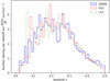Fig. 2. Number density per redshift bin of GAMA (solid blue) H15 galaxies (dashed red), and L12 galaxies (dotted green) for the limiting magnitude of r <  19.8. The bin size is Δz = 0.01.

We split the simulated lens galaxies into colour and stellar-mass samples by applying the same cuts as to the GAMA galaxies (Table 1). Figures 3 and 4 show the colour- and stellar mass distribution of observed and simulated galaxies. The colour distributions of GAMA and SAM galaxies have similar modes. However, the blue mode of the L12 SAM is more concentrated. The H15 SAM also predicts stellar mass distributions similar to the observation, while the L12 SAM predicts more galaxies with stellar masses below 9.5 × 10¹⁰ M_⊙ and fewer galaxies with stellar masses above 11 × 10¹⁰ M_⊙.

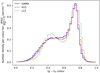Fig. 3. Number density per colour bin of GAMA (solid blue) H15 (dashed red), and L12 galaxies (dotted green) for the limiting magnitude of r <  19.8. The bin size is Δ(g − r)0 = 0.01.

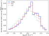Fig. 4. Number density per stellar mass bin of GAMA (solid blue) H15 (dashed red), and L12 galaxies (dotted green) for the limiting magnitude of r <  19.8. The bin size is Δlog(M*/M⊙h−2) = 0.15.

5. Results

In this section, we present our results for the physical aperture statistics ⟨𝒩𝒩M_ap⟩_phys, defined in Eq. (18). The measured angular aperture statistics ⟨𝒩𝒩M_ap⟩, which exhibit similar trends, are given in Appendix A.

The upper plot of Fig. 5 presents ⟨𝒩𝒩M_ap⟩_phys for red–red, red–blue, and blue–blue lens pairs. For the observed and both simulated data sets, the signal for red–red lens pairs is larger than for red–blue and blue–blue lens pairs. Consequently, the linear deterministic bias model of Eq. (23) suggests that the bias factor b_red of red galaxies is larger than the bias factor b_blue of blue galaxies.

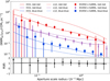Fig. 5. Upper panel: physical aperture statistics for colour-selected lens samples of the H15 galaxies (solid lines), L12 galaxies (dashed lines) and KV450 × GAMA (points). The signal is shown for red–red lens pairs (red lines and filled circles), red–blue lens pairs (purple lines and crosses), and blue–blue lens pairs (blue lines and squares). Error bars on the observational measurements are the standard deviation from jackknifing. Lower panel: ratio statistics R as given by Eq. (25) for the red and blue lens samples of KV450 × GAMA (points), the H15 SAM (solid line) and the L12 SAM (dashed line).

The linear deterministic bias model predicts that the aperture statistics for mixed red–blue lens pairs are the geometric mean of the aperture statistics for red–red and blue–blue lens pairs (see Eq. (25)). To test this prediction, we show R in the lower plot of Fig. 5. For the observed galaxies, R is consistent with unity, supporting the linear deterministic bias model. However, for scales below 0.2 h⁻¹ Mpc, the noise of the observed R is more than three times larger than R itself, which inhibits any meaningful deductions on the bias model at small scales. For the H15 model, the prediction by the linear bias model is fulfilled, while for the L12 model R is slightly larger than unity at scales below 0.2 h⁻¹ Mpc.

The SAMs give different predictions for the aperture statistics. While the ⟨𝒩𝒩M_ap⟩_phys of the H15 SAM agrees well with the observations, the signals for red–red and blue–blue lens pairs of the L12 model differ markedly. The L12 SAM predicts much larger aperture statistics for red–red pairs than the observation and significantly smaller aperture statistics for blue–blue pairs. For red–blue pairs, the signal from the L12 SAM is similar to the observed one at small scales, but too high for r >  0.3 h⁻¹ Mpc.

The difference between the SAMs is also visible in Table 2, whose upper part shows the ${\chi }_{\text{redu}}^2$ values for the different colour-selected lens pairs. We consider here p = 12 data points and define a tension between observation and simulation at the 95% confidence level (CL) if ${\chi }_{\text{redu}}^2>1.75$. For the H15 SAM, ${\chi }_{\text{redu}}^2$ is smaller than this threshold for red–red, red–blue, and blue–blue lens pairs, so there is no tension between the observation and this model. The ${\chi }_{\text{redu}}^2$ for the L12 SAM, though, are notably higher than the threshold. Consequently, the predictions by the L12 SAM do not agree with the observations for these.

Figure 6 shows the measured ⟨𝒩𝒩M_ap⟩_phys for lenses split by their stellar mass. The amplitude of the aperture statistics increases with the stellar mass of galaxies in a pair. Consequently, the bias factor increases with stellar mass. This trend exists for observed and both kinds of simulated lenses. Nevertheless, the predictions of the SAMs differ notably, with the aperture statistics obtained from the L12 SAM being substantially higher than those from the H15 SAM. The L12 SAM also deviates strongly from the observational measurements in KV450×GAMA, that agree better with the H15 SAM. The deviation of the L12 SAM from the observations is strongest for lenses with M^∗ ≤ 10^9.5 h⁻² M_⊙ and decreases for larger stellar masses.

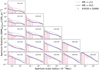Fig. 6. Physical aperture statistics for stellar mass-selected lens samples in the MR with the H15 SAM (solid blue lines), the L12 SAM (dashed grey lines), and in GAMA with KV450 sources (pink points), using the mass bins defined in Table 1. Plots on the diagonal show the signal for unmixed lens pairs, while the other plots show the signal for mixed lens pairs. Error bars are the standard deviation from jackknife resampling.

To quantify the deviation, we list the ${\chi }_{\text{redu}}^2$ of the aperture statistics measured in the H15 and L12 SAM in the lower part of Table 3. Again, a ${\chi }_{\text{redu}}^2>1.75$ indicates a tension at the 95% CL. The L12 SAM disagrees with the observation for all lens samples. The ${\chi }_{\text{redu}}^2$ of the H15 SAM, though, are smaller than 1.75 for all but one correlation. The only tension exists for the correlation of lenses from stellar-mass samples m1 and m4, driven by differences at r ≲ 0.2 h⁻¹ Mpc, where the H15 SAM underestimates ⟨𝒩𝒩M_ap⟩_phys.

Finally, we test for systematic effects by considering the B-mode ⟨𝒩𝒩M_⊥⟩. Table 3 compares the S/Ns, defined by Eq. (47), of ⟨𝒩𝒩M_ap⟩_phys with those of the B-modes ⟨𝒩𝒩M_⊥⟩ for all observed lens pairs. The S/Ns of ⟨𝒩𝒩M_⊥⟩ are considerably smaller than the S/Ns of the ⟨𝒩𝒩M_ap⟩_phys, and they are consistent with a vanishing B-mode.

6. Discussion

We evaluated the SAM by H15 and the SAM by L12 by comparing their G3L predictions to measurements with KiDS, VIKING and GAMA. For this, we applied the improved estimator for the G3L three-point correlation function by L20 and measured aperture statistics for mixed and unmixed lens galaxy pairs from colour- or stellar-mass-selected lens samples.

Our measurements show a higher S/N than previous studies of G3L, due to the use of an improved estimator for G3L and new data. As shown in L20, redshift weighting increases the S/N of the aperture statistics by 35% on mock data with a similar lens- and redshift distribution as in our observation. We also extended the considered scales. Therefore, we could probe the predictions of the SAMs well inside of dark matter halos at lengths below 1 h⁻¹ Mpc. These ranges are particularly interesting for testing galaxy formation models because the principal variations between different SAMs are the assumptions on phenomena, whose effects are most substantial at small scales, such as star formation, stellar and AGN feedback and environmental processes (Guo et al. 2016).

The aperture statistics are larger for red–red lens pairs than for red–blue or blue–blue lens pairs, which indicates that red galaxies have higher bias factors than blue galaxies. We also found that the bias factor increases with stellar mass. These results support the general expectation that redder and more massive galaxies have higher bias factors, which has been found in multiple studies (e.g. Zehavi et al. 2002; Sheldon et al. 2004; Simon & Hilbert 2018; Saghiha et al. 2017).

The predictions by the H15 SAM for aperture statistics of colour-selected lens samples agree with the observations at the 95% CL. The signal predicted by the L12 SAM, though, deviates significantly from the observed G3L signal, being too high for red–red and red–blue, and too low for blue–blue pairs.

This deviation could be due to an overproduction of red galaxies in massive halos by the L12 SAM. As shown by Watts & Schneider (2005), the G3L signal increases if more lens pairs reside in massive halos, so the relatively high ⟨𝒩𝒩M_ap⟩_phys indicates that in the L12 SAM massive halos contain too many pairs of red galaxies. This interpretation is supported by studies by Baldry et al. (2006) of the Bower et al. (2006) SAM, on which the L12 SAM is based. They compare the fraction of red galaxies in the SAM with observations by the SDSS and found that the SAM predicts too many red galaxies, especially in regions of high surface mass density.

Font et al. (2008) accredite the overproduction of red satellite galaxies to excessive tidal interactions and ram pressure stripping in the L12 SAM. This process decreases the amount of gas in satellite galaxies inside halos and thereby inhibits their star formation. Consequently, the stripped galaxies become redder, so the fraction of red galaxies increases, while the number of blue galaxies decreases. This effect could explain the low aperture statistics for blue–blue lens pairs in the Lagos et al. (2012) SAM, as fewer blue galaxies remain inside massive halos.

The aperture statistics for the stellar-mass-selected samples measured in the observation agree with the H15 SAM at the 95% CL except for one sample. This finding is consistent with the conclusion by Saghiha et al. (2017), although their study is limited to angular scales between 1′ and 10′, did not consider mixed lens pairs and had a lower S/N due to the effect of chance lens pairs.

The H15 SAM agrees with the observations at the 95% CL for all but the correlation of m1 and m4 lens galaxies. This difference is driven mainly by a low signal by the SAM at scales below 0.2 h⁻¹ Mpc. At these scales, the SAM also gives lower predictions for ⟨𝒩𝒩M_ap⟩ than the observations for m1–m2, m1–m3, and m2–m2 lens pairs. This trend could indicate that the SAM underpredicts G3L at small scales for low stellar masses. A possible reason is the limited resolution of the MR. The MRs softening length is 5 h⁻¹kpc, so its spatial resolution is in the order of tens of kiloparsec (Vogelsberger et al. 2020). Therefore, the difference between the aperture statistics in the H15 SAM and the observation at small scales might be due to the limited resolution.

The L12 SAM disagrees with the observations for all considered stellar-mass samples at the 95% CL, and its predicted signal is significantly larger. The tension increases for lenses with lower stellar mass and is more prominent at smaller scales.

This tension might be due to inaccurate stellar masses of the simulated lens galaxies. If the SAM assigns too low stellar masses, galaxies from a higher stellar mass bin are incorrectly assigned to a lower mass bin, for example into m2 instead of m3. The SAM then overestimates the aperture statistics, because the bias factors of galaxies with larger stellar masses are higher. The choice of initial mass function could cause different stellar-mass assignments by the SAMs. While the H15 SAM used the same initial mass function as the observations (Chabrier 2003), the L12 SAM assumes the initial mass function by Kennicutt (1983). Therefore, the stellar masses of the observation and the L12 might be inconsistent with each other.

Another cause for the tension of the L12 SAM with the observation could be an overproduction of satellite galaxies inside massive halos. This interpretation agrees with Saghiha et al. (2017), who find that the satellite fraction and mean halo masses for the L12 SAM is higher than for the H15 SAM. The tension between the L12 SAM and the observation increases for lower stellar masses and smaller scales, indicating that especially galaxies with low stellar mass are overproduced by the SAM and that their fraction rises closer to the centre of their dark matter halo. An excess of galaxies with small stellar masses would be consistent with excessive galaxy interactions inside halos. This finding, therefore, fits with the interpretation of the high G3L signal for red–red lens pairs in the SAM as caused by excessive ram pressure stripping.

We presented the first measurements of G3L for mixed lens pairs and used the aperture statistics for red–blue lens pairs to test the linear deterministic bias model. This bias model predicts that the aperture statistics for mixed lens pairs is the geometric mean of the signals for equal lens pairs. Our observational measurements are consistent with this prediction, although the signal is too noisy at scales below 0.2 h⁻¹ Mpc for meaningful constraints on the bias model.

The aperture statistics for mixed lens pairs are also useful to constrain the correlations of different galaxy populations inside the same dark matter halos. For example, the measured aperture statistics for red–blue lens pairs indicate that lens galaxies of different samples co-populate the same halos, as the signal would decrease at sub-Mpc scales due to a vanishing 1-halo term. Modelling of mixed-pair G3L in the context of the halo model will provide further insights into the correlation of galaxy populations inside halos. In contrast, GGL, which is only sensitive to the mean number of lenses inside halos and hence blind to the way mixed lens pairs populate halos, cannot yield the same information.

A compelling future study would be investigating whether full hydrodynamical simulations predict G3L with the same accuracy as the H15 SAM. Such a study would complement previous comparisons of GGL in hydrodynamical simulations to observations, for example by Velliscig et al. (2017) for the EAGLE simulation to KiDS and GAMA data, or Gouin et al. (2019) for the Horizon-AGN simulation to CFHTLenS and the Baryon Oscillation Spectroscopic Survey. While these studies conclude that the GGL predictions of these simulations agree with the observations, the same is not necessarily true for G3L, which depends on the correlation of matter and galaxy pairs.

Acknowledgments

LL is a member of and received financial support for this research from the International Max Planck Research School (IMPRS) for Astronomy and Astrophysics at the Universities of Bonn and Cologne. CH acknowledges support from the European Research Council under grant number 647112, and support from the Max Planck Society and the Alexander von Humboldt Foundation in the framework of the Max Planck-Humboldt Research Award endowed by the Federal Ministry of Education and Research. H. Hildebrandt is supported by a Heisenberg grant of the Deutsche Forschungsgemeinschaft (Hi 1495/5-1) as well as an ERC Consolidator Grant (No. 770935). AK acknowledges support from Vici grant 639.043.512, financed by the Netherlands Organisation for Scientific Research (NWO). CS acknowledges support from the Agencia Nacional de Investigación y Desarrollo (ANID) through grant FONDECYT Iniciación 11191125. AHW is supported by a European Research Council Consolidator Grant (No. 770935). Based on data products from observations made with ESO Telescopes at the La Silla Paranal Observatory under programme IDs 177.A-3016, 177.A-3017, 177.A-3018, 179.A-2004, 298.A-5015. We also use products from the GAMA survey. GAMA is a joint European-Australasian project based around a spectroscopic campaign using the Anglo-Australian Telescope. The GAMA input catalogue is based on data taken from the Sloan Digital Sky Survey and the UKIRT Infrared Deep Sky Survey. Complementary imaging of the GAMA regions is being obtained by several independent survey programmes including GALEX MIS, VST KiDS, VISTA VIKING, WISE, Herschel-ATLAS, GMRT and ASKAP providing UV to radio coverage. GAMA is funded by the STFC (UK), the ARC (Australia), the AAO, and the participating institutions. The GAMA website is http://www.gama-survey.org/. Author contributions: all authors contributed to the development and writing of this paper. The authorship list is given in two groups: The lead authors (LL, PSi, PS), followed by an alphabetical list of contributors to either the scientific analysis or the data products.

References

Appendix A: Results for aperture statistics in angular units

For completeness, we show here our results for the angular aperture statistics ⟨𝒩𝒩M_ap⟩, for colour-selected lens samples (Fig. A.1) and stellar-mass-selected lens samples (Fig. A.2). The ⟨𝒩𝒩M_ap⟩ exhibit similar trends to the ⟨𝒩𝒩M_ap⟩_phys (see Sect 5). In particular, ⟨𝒩𝒩M_ap⟩ also increases with the lenses stellar masses and is larger for red–red than for red–blue or blue–blue lens galaxies. Furthermore, the predictions by the H15 SAM agrees well with the observed ⟨𝒩𝒩M_ap⟩, while the L12 SAM expects too large aperture statistics, especially for low stellar-mass galaxies.

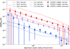Fig. A.1. Aperture statistics in angular units for colour-selected lens samples of the H15 galaxies (solid lines), L12 galaxies (dashed lines) and KV450 × GAMA (points). The signal is shown for red–red lens pairs (red lines and filled circles), red–blue lens pairs (purple lines and crosses), and blue–blue lens pairs (blue lines and squares). Error bars on the observational measurements are the standard deviation from jackknifing.

The agreement of the H15 SAM and the discrepancy of the L12 SAM with the observations is supported by the ${\chi }_{\text{redu}}^2$ of the SAMs predictions for ⟨𝒩𝒩M_ap⟩, presented in Table A.1. The H15 SAM disagrees with the observations only for the correlation of m1 and m4 galaxies at the 95% CL, while the L12 SAM is in tension with the observation for all samples.

Note, that while the measurements of ⟨𝒩𝒩M_ap⟩ do not depend on the choice of cosmology, they change with the lens redshift distribution. Comparing ⟨𝒩𝒩M_ap⟩ measured in different observational surveys requires, therefore, careful consideration of the survey’s selection functions.

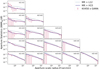Fig. A.2. Angular aperture statistics for stellar mass-selected lens samples in the MR with the H15 SAM (solid blue lines), the L12 SAM (dashed grey lines), and in GAMA with KV450 sources (pink points), using the mass bins defined in Table 1. Plots on the diagonal show the signal for unmixed lens pairs, while the other plots show the signal for mixed lens pairs. Error bars are the standard deviation from jackknife resampling.

All Tables

All Figures

Fig. 1. Geometry of a G3L configuration with one source and two lens galaxies; adapted from Schneider & Watts (2005). The two lens galaxies are at angular positions θ1 and θ2 on the sky; the source galaxy is at θ. The separation vectors ϑ1 and ϑ2 of the lenses from the source have lengths ϑ1 and ϑ2, as well as polar angles φ1 and φ2. The angle between ϑ1 and ϑ2 is the opening angle ϕ. The tangential shear of the source galaxy is measured with respect to the dashed line, which is the bisector of ϕ.

In the text

	Fig. 2. Number density per redshift bin of GAMA (solid blue) H15 galaxies (dashed red), and L12 galaxies (dotted green) for the limiting magnitude of r <  19.8. The bin size is Δz = 0.01.
In the text

	Fig. 3. Number density per colour bin of GAMA (solid blue) H15 (dashed red), and L12 galaxies (dotted green) for the limiting magnitude of r <  19.8. The bin size is Δ(g − r)0 = 0.01.
In the text

	Fig. 4. Number density per stellar mass bin of GAMA (solid blue) H15 (dashed red), and L12 galaxies (dotted green) for the limiting magnitude of r <  19.8. The bin size is Δlog(M*/M⊙h−2) = 0.15.
In the text

Fig. 5. Upper panel: physical aperture statistics for colour-selected lens samples of the H15 galaxies (solid lines), L12 galaxies (dashed lines) and KV450 × GAMA (points). The signal is shown for red–red lens pairs (red lines and filled circles), red–blue lens pairs (purple lines and crosses), and blue–blue lens pairs (blue lines and squares). Error bars on the observational measurements are the standard deviation from jackknifing. Lower panel: ratio statistics R as given by Eq. (25) for the red and blue lens samples of KV450 × GAMA (points), the H15 SAM (solid line) and the L12 SAM (dashed line).

In the text

Fig. 6. Physical aperture statistics for stellar mass-selected lens samples in the MR with the H15 SAM (solid blue lines), the L12 SAM (dashed grey lines), and in GAMA with KV450 sources (pink points), using the mass bins defined in Table 1. Plots on the diagonal show the signal for unmixed lens pairs, while the other plots show the signal for mixed lens pairs. Error bars are the standard deviation from jackknife resampling.

In the text

Fig. A.1. Aperture statistics in angular units for colour-selected lens samples of the H15 galaxies (solid lines), L12 galaxies (dashed lines) and KV450 × GAMA (points). The signal is shown for red–red lens pairs (red lines and filled circles), red–blue lens pairs (purple lines and crosses), and blue–blue lens pairs (blue lines and squares). Error bars on the observational measurements are the standard deviation from jackknifing.

In the text

Fig. A.2. Angular aperture statistics for stellar mass-selected lens samples in the MR with the H15 SAM (solid blue lines), the L12 SAM (dashed grey lines), and in GAMA with KV450 sources (pink points), using the mass bins defined in Table 1. Plots on the diagonal show the signal for unmixed lens pairs, while the other plots show the signal for mixed lens pairs. Error bars are the standard deviation from jackknife resampling.

In the text

References

- Anderson, T. W. 2003, An Introduction to Multivariate Statistical Analysis, 3rd edn. (Hoboken, NJ: Wiley-Interscience) [Google Scholar]
- Baldry, I. K., Balogh, M. L., Bower, R. G., et al. 2006, MNRAS, 373, 469 [NASA ADS] [CrossRef] [Google Scholar]
- Baldry, I. K., Driver, S. P., Loveday, J., et al. 2012, MNRAS, 421, 621 [NASA ADS] [Google Scholar]
- Bartelmann, M., & Schneider, P. 2001, Phys. Rep., 340, 291 [NASA ADS] [CrossRef] [Google Scholar]
- Blanton, M. R., & Roweis, S. 2007, AJ, 133, 734 [NASA ADS] [CrossRef] [Google Scholar]
- Bower, R. G., Benson, A. J., Malbon, R., et al. 2006, MNRAS, 370, 645 [NASA ADS] [CrossRef] [Google Scholar]
- Bruzual, G., & Charlot, S. 2003, MNRAS, 344, 1000 [NASA ADS] [CrossRef] [Google Scholar]
- Calzetti, D., Armus, L., Bohlin, R. C., et al. 2000, ApJ, 533, 682 [NASA ADS] [CrossRef] [Google Scholar]
- Chabrier, G. 2003, PASP, 115, 763 [Google Scholar]
- Clampitt, J., Miyatake, H., Jain, B., & Takada, M. 2016, MNRAS, 457, 2391 [NASA ADS] [CrossRef] [Google Scholar]
- Crain, R. A., Schaye, J., Bower, R. G., et al. 2015, MNRAS, 450, 1937 [NASA ADS] [CrossRef] [Google Scholar]
- de Jong, J. T. A., Verdoes Kleijn, G. A., Boxhoorn, D. R., et al. 2015, A&A, 582, A62 [NASA ADS] [CrossRef] [EDP Sciences] [Google Scholar]
- de Jong, J. T. A., Verdoes Kleijn, G. A., Erben, T., et al. 2017, A&A, 604, A134 [NASA ADS] [CrossRef] [EDP Sciences] [Google Scholar]
- Driver, S. P., Norberg, P., Baldry, I. K., et al. 2009, Astron. Geophys., 50, 12 [Google Scholar]
- Driver, S. P., Hill, D. T., Kelvin, L. S., et al. 2011, MNRAS, 413, 971 [NASA ADS] [CrossRef] [Google Scholar]
- Dvornik, A., Hoekstra, H., Kuijken, K., et al. 2018, MNRAS, 479, 1240 [NASA ADS] [CrossRef] [Google Scholar]
- Edge, A., Sutherland, W., Kuijken, K., et al. 2013, The Messenger, 154, 32 [NASA ADS] [Google Scholar]
- Epps, S. D., & Hudson, M. J. 2017, MNRAS, 468, 2605 [NASA ADS] [CrossRef] [Google Scholar]
- Erben, T., Schirmer, M., Dietrich, J. P., et al. 2005, Astron. Nachr., 326, 432 [NASA ADS] [CrossRef] [Google Scholar]
- Farrow, D. J., Cole, S., Norberg, P., et al. 2015, MNRAS, 454, 2120 [NASA ADS] [CrossRef] [Google Scholar]
- Font, A. S., Bower, R. G., McCarthy, I. G., et al. 2008, MNRAS, 389, 1619 [NASA ADS] [CrossRef] [Google Scholar]
- Gouin, C., Gavazzi, R., Pichon, C., et al. 2019, A&A, 626, A72 [NASA ADS] [CrossRef] [EDP Sciences] [Google Scholar]
- Guo, Q., White, S., Boylan-Kolchin, M., et al. 2011, MNRAS, 413, 101 [NASA ADS] [CrossRef] [Google Scholar]
- Guo, Q., Gonzalez-Perez, V., Guo, Q., et al. 2016, MNRAS, 461, 3457 [NASA ADS] [CrossRef] [Google Scholar]
- Hartlap, J., Simon, P., & Schneider, P. 2007, A&A, 464, 399 [NASA ADS] [CrossRef] [EDP Sciences] [Google Scholar]
- Henriques, B. M. B., White, S. D. M., Thomas, P. A., et al. 2015, MNRAS, 451, 2663 [NASA ADS] [CrossRef] [Google Scholar]
- Henriques, B. M. B., White, S. D. M., Thomas, P. A., et al. 2017, MNRAS, 469, 2626 [Google Scholar]
- Heymans, C., Van Waerbeke, L., Miller, L., et al. 2012, MNRAS, 427, 146 [NASA ADS] [CrossRef] [Google Scholar]
- Hilbert, S., Hartlap, J., White, S. D. M., & Schneider, P. 2009, A&A, 499, 31 [NASA ADS] [CrossRef] [EDP Sciences] [Google Scholar]
- Hildebrandt, H., Choi, A., Heymans, C., et al. 2016, MNRAS, 463, 635 [NASA ADS] [CrossRef] [Google Scholar]
- Hildebrandt, H., Viola, M., Heymans, C., et al. 2017, MNRAS, 465, 1454 [Google Scholar]
- Hildebrandt, H., Köhlinger, F., van den Busch, J. L., et al. 2020, A&A, 633, A69 [NASA ADS] [CrossRef] [EDP Sciences] [Google Scholar]
- Kaiser, N. 1984, ApJ, 284, L9 [NASA ADS] [CrossRef] [Google Scholar]
- Kannawadi, A., Hoekstra, H., Miller, L., et al. 2019, A&A, 624, A92 [NASA ADS] [CrossRef] [EDP Sciences] [Google Scholar]
- Kaviraj, S., Laigle, C., Kimm, T., et al. 2017, MNRAS, 467, 4739 [NASA ADS] [Google Scholar]
- Kennicutt, R. C., Jr. 1983, ApJ, 272, 54 [NASA ADS] [CrossRef] [EDP Sciences] [Google Scholar]
- Kuijken, K., Heymans, C., Hildebrandt, H., et al. 2015, MNRAS, 454, 3500 [NASA ADS] [CrossRef] [Google Scholar]
- Lagos, C. D. P., Bayet, E., Baugh, C. M., et al. 2012, MNRAS, 426, 2142 [NASA ADS] [CrossRef] [Google Scholar]
- Landy, S. D., & Szalay, A. S. 1993, ApJ, 412, 64 [NASA ADS] [CrossRef] [Google Scholar]
- Linke, L., Simon, P., Schneider, P., & Hilbert, S. 2020, A&A, 634, A13 [NASA ADS] [CrossRef] [EDP Sciences] [Google Scholar]
- Liske, J., Baldry, I. K., Driver, S. P., et al. 2015, MNRAS, 452, 2087 [NASA ADS] [CrossRef] [Google Scholar]
- Maraston, C. 2005, MNRAS, 362, 799 [NASA ADS] [CrossRef] [Google Scholar]
- Mead, J. M. G., King, L. J., & McCarthy, I. G. 2010, MNRAS, 401, 2257 [NASA ADS] [CrossRef] [Google Scholar]
- Miller, L., Heymans, C., Kitching, T. D., et al. 2013, MNRAS, 429, 2858 [Google Scholar]
- Nelson, D., Springel, V., Pillepich, A., et al. 2019, Comput. Astrophys. Cosmol., 6, 2 [Google Scholar]
- Planck Collaboration I. 2020, A&A, in press, https://doi.org/10.1051/0004-6361/201833880 [Google Scholar]
- Saghiha, H., Simon, P., Schneider, P., & Hilbert, S. 2017, A&A, 601, A98 [NASA ADS] [CrossRef] [EDP Sciences] [Google Scholar]
- Schirmer, M. 2013, ApJS, 209, 21 [NASA ADS] [CrossRef] [Google Scholar]
- Schneider, P. 2003, A&A, 408, 829 [NASA ADS] [CrossRef] [EDP Sciences] [Google Scholar]
- Schneider, P., & Watts, P. 2005, A&A, 432, 783 [NASA ADS] [CrossRef] [EDP Sciences] [Google Scholar]
- Sheldon, E. S., Johnston, D. E., Frieman, J. A., et al. 2004, AJ, 127, 2544 [NASA ADS] [CrossRef] [Google Scholar]
- Simon, P., & Hilbert, S. 2018, A&A, 613, A15 [NASA ADS] [CrossRef] [EDP Sciences] [Google Scholar]
- Simon, P., Watts, P., Schneider, P., et al. 2008, A&A, 479, 655 [NASA ADS] [CrossRef] [EDP Sciences] [Google Scholar]
- Simon, P., Erben, T., Schneider, P., et al. 2013, MNRAS, 430, 2476 [NASA ADS] [CrossRef] [EDP Sciences] [Google Scholar]
- Simon, P., Saghiha, H., Hilbert, S., et al. 2019, A&A, 622, A104 [NASA ADS] [CrossRef] [EDP Sciences] [Google Scholar]
- Springel, V., White, S. D. M., Jenkins, A., et al. 2005, Nature, 435, 629 [NASA ADS] [CrossRef] [PubMed] [Google Scholar]
- Szapudi, I., & Szalay, A. S. 1998, ApJ, 494, L41 [NASA ADS] [CrossRef] [Google Scholar]
- Taylor, E. N., Hopkins, A. M., Baldry, I. K., et al. 2015, MNRAS, 446, 2144 [NASA ADS] [CrossRef] [Google Scholar]
- Tonry, J. L., Blakeslee, J. P., Ajhar, E. A., & Dressler, A. 2000, ApJ, 530, 625 [NASA ADS] [CrossRef] [Google Scholar]
- Velliscig, M., Cacciato, M., Hoekstra, H., et al. 2017, MNRAS, 471, 2856 [NASA ADS] [CrossRef] [Google Scholar]
- Venemans, B. P., Verdoes Kleijn, G. A., Mwebaze, J., et al. 2015, MNRAS, 453, 2259 [NASA ADS] [CrossRef] [Google Scholar]
- Vogelsberger, M., Genel, S., Springel, V., et al. 2014, MNRAS, 444, 1518 [NASA ADS] [CrossRef] [Google Scholar]
- Vogelsberger, M., Marinacci, F., Torrey, P., & Puchwein, E. 2020, Nat. Rev. Phys., 2, 42 [CrossRef] [Google Scholar]
- Watts, P., & Schneider, P. 2005, IAU Symp., 225, 243 [NASA ADS] [Google Scholar]
- Wright, A. H., Robotham, A. S. G., Bourne, N., et al. 2016, MNRAS, 460, 765 [NASA ADS] [CrossRef] [Google Scholar]
- Wright, A. H., Robotham, A. S. G., Driver, S. P., et al. 2017, MNRAS, 470, 283 [NASA ADS] [CrossRef] [Google Scholar]
- Wright, A. H., Hildebrandt, H., Kuijken, K., et al. 2019, A&A, 632, A34 [NASA ADS] [CrossRef] [EDP Sciences] [Google Scholar]
- Xia, Q., Robertson, N., Heymans, C., et al. 2020, A&A, 633, A89 [NASA ADS] [CrossRef] [EDP Sciences] [Google Scholar]
- Zehavi, I., Blanton, M. R., Frieman, J. A., et al. 2002, ApJ, 571, 172 [NASA ADS] [CrossRef] [Google Scholar]