© The Authors 2024

1 Introduction

Cosmic shear, the correlations between galaxy shapes due to the weak gravitational lensing by the cosmic large-scale structure, is a popular and constraining probe of cosmology. Cosmic shear surveys such as the Dark Energy Survey (DES, Abbott et al. 2016; Becker et al. 2016), the Kilo-Degree Survey (KiDS, Kuijken et al. 2015), or the Hyper-Suprime-Cam survey (HSC, Aihara et al. 2018) constrain the parameter $S_8={\sigma }_8\sqrt{{\mathrm{\Omega }}_{\mathrm{m}}/0.3}$, which is a combination of the matter density parameter Ω_m and the clustering parameter σ₈, at 2–4 per cent (Asgari et al. 2021; Amon et al. 2022; Secco et al. 2022; Dalal et al. 2023; Li et al. 2023). Soon, even more extensive and deeper surveys such as Euclid (Laureijs et al. 2011; Euclid Collaboration 2024), Vera C. Rubin Observatory’s Legacy Survey of Space and Time (LSST, Ivezić et al. 2019) or the Nancy Grace Roman space telescope (Akeson et al. 2019) will use cosmic shear in combination with the correlations of galaxy positions to not only better constrain Ω_m and σ₈, but also determine the time evolution of dark energy (The LSST Dark Energy Science Collaboration 2018; Euclid Collaboration 2020). Arguably, cosmic shear is now entering its most exciting phase as a probe of our Universe.

While the increasing size of the data sets provides more and more precision, the accuracy of theoretical predictions also needs to be updated. For this, several astrophysical effects that impact cosmic shear measurements must be understood. One such effect is the alignment between the intrinsic shapes of galaxies, the so-called intrinsic alignment (IA, Lamman et al. 2024; Troxel & Ishak 2015; Joachimi et al. 2015). IA occurs due to the formation of galaxies within the dark matter-dominated gravitational field (Catelan et al. 2001). Elliptical galaxies tend to be aligned with the gravitational tidal field, leading to a radial alignment with respect to matter overdensities (Kiessling et al. 2015). These alignments add to the observed shape correlations and thus contaminate the cosmic shear signal.

If IA is not taken into account in cosmic shear analyses, inferred parameters can be severely biased (Hirata et al. 2007; Kirk et al. 2015). Therefore, cosmic shear analyses commonly incorporate a description for IA in their model with some free parameters that are constrained in the inference simultaneously with the cosmological parameters.

Several IA models have been proposed for this purpose. A relatively simple model is the non-linear linear alignment (NLA) model by Bridle & King (2007). This empirical model assumes that the power spectrum of galaxy shapes is linearly related to the non-linear matter power spectrum via a free parameter A_IA describing the amplitude of the correlation. While it is only a phenomenological description, it fits well to IA measurements for red central galaxies at large scales (Singh et al. 2015). There are also other more physically motivated models, such as the Tidal Alignment and Tidal Torque (TATT) model (Blazek et al. 2019), which allows galaxies to not align solely with the gravitational tidal field but also the tidal torque and includes a density weighting term. Alternatively, there are halo model descriptions (Schneider & Bridle 2010; Fortuna et al. 2021), which explicitly distinguish between central and satellite galaxies inside dark matter halos. Other models are based on perturbative approaches (Vlah et al. 2020; Maion et al. 2024; Chen & Kokron 2024). The accuracy of the models depends on the considered physical scales and galaxy samples. It is currently unclear which IA models offer the best trade-off between model complexity and accuracy for any given analysis. For example, there is no clear observational evidence yet on whether the more complex TATT or the simpler NLA model are more appropriate for cosmological analyses (DES and KiDS Collaboration: Abbott et al. 2023).

However, the choice of model can impact cosmological parameter constraints. DES and KiDS Collaboration: Abbott et al. (2023) find in a combined analysis of DES and KiDS that using the TATT instead of the NLA model can lower the inferred value for S₈ by almost 3 per cent, corresponding to a shift by 0.9σ. Consequently, it is paramount to test IA models independently of cosmic shear measurements to find an appropriate model. Furthermore, independent constraints of IA model parameters can be used as priors for cosmic shear analyses, significantly tightening constraints on other parameters (Johnston et al. 2019).

IA studies so far have been mainly concerned with secondorder correlations of matter overdensity and intrinsic galaxy shapes. Mostly the shape-shape and density-shape correlations are constrained (e.g. Joachimi et al. 2011; Singh et al. 2015; Singh & Mandelbaum 2016; Johnston et al. 2019; Fortuna et al. 2021; Johnston et al. 2021; Samuroff et al. 2023). For several reasons, though, it has become increasingly interesting to study higher-order statistics (HOS), for example third-order correlations. For example, while current IA models are well-designed to describe second-order IA correlations, it is an important consistency check to see whether they also match higher-order correlations. An example of such a test is carried out by Pyne et al. (2022), who measure the IA power- and bispectrum in simulations and find that the same model parameters could describe both. Furthermore, HOS depend differently on both cosmological and IA parameters. Combining second-order and HOS can reduce parameter degeneracies and lead to better constraints (e.g. Burger et al. 2024; Euclid Collaboration 2023). Adding higher-order information can also help in self-calibrating systematic effects such as IA (Pyne & Joachimi 2021). Analyses similar to these are vital to optimally use the data sets of Euclid and LSST, but they can only be performed if we can ensure we understand how systematic effects such as IA behave for third-order statistics. As shown by Semboloni et al. (2008) using cosmological simulations, third-order correlations of intrinsic galaxy shapes and the matter field can significantly impact analysis of third-order cosmic shear and contribute as much as 15% of the signal for surveys with a median redshift of 0.7. Consequently, we must include IA in the modelling of the third-order cosmic shear signal and demonstrate that our models can accurately describe higher-order correlations of the matter overdensity and the intrinsic shapes of galaxies.

In this paper, we take the first step towards this by reporting the first detection of third-order intrinsic alignment correlations in the low-redshift (LOWZ) galaxy sample from the Sloan Digital Sky Survey (SDSS) Baryon Oscillation Spectroscopic Survey (BOSS) survey. This sample contains spectroscopically observed luminous red galaxies (LRGs) at redshifts below 0.4. For this sample, Singh et al. (2015) measured second-order correlations between the matter density and the shapes and between shapes of different galaxies. The measurement was conducted by using the positions of galaxies as tracers for the matter distribution and comparing them pairwise to the galaxies’ shapes. We followed in their footsteps by comparing the positions of galaxy pairs with the shape of a third galaxy, thus measuring the density-density-shape correlation. This correlation was then compared to predictions by the Marenostrum Institut de Ciències de l’Espai (MICE) cosmological simulation and an analytical NLA-based model.

This paper is structured as follows. In Sect. 2, we define fundamental notations, describe the third-order intrinsic alignment correlation function and relate it to the matter-matter-shape bispectrum. In Sect. 3, we describe our estimator for the correlation function and our covariance estimate. Section 4 describes the observed and simulated data sets. The measurements and comparisons to the analytical model are presented in Sect. 5. We conclude with a discussion in Sect. 6.

2 Theoretical background and modelling

2.1 Basic quantities and definitions

In the weak gravitational lensing limit (see e.g. Bartelmann & Schneider 2001 for a review), the observed ellipticity ε(ϑ) of a source galaxy at angular position ϑ is determined by its intrinsic ellipticity ϑ_I(ϑ) and the weak lensing shear γ(ϑ), both of which are complex quantities. In weak lensing, |γ| ≪ 1, and, $$ϵ(\mathit{\vartheta })={ϵ}_{\mathrm{I}}(\mathit{\vartheta })+\gamma (\mathit{\vartheta }).$$(1)

Under the flat sky approximation, the shear is related to the lensing convergence κ via the Kaiser-Squires relation (Kaiser & Squires 1993) $$\tilde{\gamma }(\mathit{\ell })={\mathrm{e}}^{2\mathrm{i}{\varphi }_{\ell }}\tilde{\kappa }(\mathit{\ell }),$$(2)

where the tilde denotes Fourier transform and ϕ_ℓ is the polar angle of the angular frequency ℓ. Analogously, we can define an ‘intrinsic alignment (IA) convergence’ κ_I, which describes the convergence that would cause a shear equivalent to the intrinsic source ellipticity via $${\widetilde{ϵ}}_{\mathrm{I}}(\mathit{\ell })={\mathrm{e}}^{2\mathrm{i}{\varphi }_{\ell }}\widetilde{{\kappa }_{\mathrm{I}}}(\mathit{\ell }).$$(3)

For source galaxies distributed with a probability distribution p(χ) with comoving distance χ, κ(ϑ) is a weighted integral over the κ(ϑ, χ) at each χ, $$\begin{array}{rl}\kappa (\mathit{\vartheta })& =\int \mathrm{d}\chi p(\chi )\kappa (\mathit{\vartheta },\chi )\\ & =\int \mathrm{d}\chi p(\chi )\int \mathrm{d}{\chi }^{\mathrm{\prime }}W(\chi ,{\chi }^{\mathrm{\prime }})\delta ({\chi }^{\mathrm{\prime }}\mathit{\vartheta },{\chi }^{\mathrm{\prime }}),\end{array}$$(4)

where we assumed a flat Universe, δ(χϑ, χ) is the matter density contrast at angular position ϑ and distance χ, and W is the lensing efficiency given by $$W(\chi ,{\chi }^{\mathrm{\prime }})=\frac{3H_0^2{\mathrm{\Omega }}_{\mathrm{m}}}{2c^2}\frac{{\chi }^{\mathrm{\prime }}(\chi -{\chi }^{\mathrm{\prime }})}{\chi a({\chi }^{\mathrm{\prime }})},$$(5)

where H₀ is the Hubble constant, Ω_m is the matter density parameter, and a(χ) is the scale factor at co-moving distance χ. The κ₁ can be related to a density contrast δ_I, which would cause a shear equivalent to the intrinsic galaxy ellipticity, $${\kappa }_{\mathrm{I}}(\mathit{\vartheta })=\int \mathrm{d}\chi p(\chi ){\delta }_{\mathrm{I}}(\chi \mathit{\vartheta },\chi ).$$(6)

We are interested in correlations between the intrinsic ellipticity field δ_I and the matter density contrast δ. To study these correlations, we use galaxy positions as tracers of the matter field. Their distribution is characterised by their threedimensional number density n(χϑ, χ) at angular position ϑ and distance χ. This density is related to the galaxy number density contrast δ_g by $$n(\chi \mathit{\vartheta },\chi )=\overline{n}(\chi )[{\delta }_g(\chi \mathit{\vartheta },\chi )+1],$$(7)

where $\overline{n}(\chi )$ is the average number density at comoving distance χ. From this, we also define the projected, two-dimensional galaxy number density N(ϑ) as $$N(\mathit{\vartheta })=\int \mathrm{d}\chi p(\chi )n(\chi \mathit{\vartheta },\chi ),$$(8)

whose average we denote as $\overline{N}$.

2.2 Intrinsic alignment correlation functions

Since the intrinsic ellipticity of an individual galaxy is unknown, its observed ellipticity alone does not contain usable cosmological information. Instead, one needs to consider the correlation functions of the ellipticities. The most commonly used ones are the second-order correlations, either of the ellipticities ε with themselves (i.e. ‘cosmic shear’) or between ellipticities and the galaxy number density N (i.e. ‘galaxy-galaxy-lensing’). Here, though, we are interested in third-order correlation functions involving galaxy shapes. For this, we have, in principle, three choices: correlating the ellipticities at three different positions (‘third-order cosmic shear’, Schneider & Lombardi 2003)), the ellipticities at two positions with the galaxy number density at a third position, or the ellipticity at one position with the number density at two different positions (‘galaxy-galaxy-galaxy lensing’, G3L, Schneider & Watts 2005). The last of these, so-called shape-lens-lens G3L, has the highest signal-to-noise ratio (Simon et al. 2012), so we concentrate on this.

Additionally, one can also construct the correlation between the galaxy number density at three different positions (‘thirdorder galaxy clustering’) (Scoccimarro & Couchman 2001; Takada & Jain 2003). While this correlation does not include any information on the shapes or IA of the galaxies, it is a useful statistic of the cosmic large-scale structure, has been measured in several galaxy surveys (e.g Marín et al. 2013; Slepian et al. 2017) and can improve constraints from cosmological inference (Yankelevich & Porciani 2019; Eggemeier et al. 2021; Ivanov et al. 2023)

In general, the correlation function for shape-lens-lens G3L is $$G^{\mathrm{\prime }}({\mathit{\vartheta }}_1,{\mathit{\vartheta }}_2)=\frac{1}{{\overline{N}}^2}⟨N(\mathit{\theta }+{\mathit{\vartheta }}_1)N(\mathit{\theta }+{\mathit{\vartheta }}_2)ϵ(\mathit{\theta }){\mathrm{e}}^{-\mathrm{i}({\varphi }_1+{\varphi }_2)}⟩,$$(9)

where the ϑ_i are the angular separations between the lens galaxies and the shape tracing galaxy, with polar angles ϕ_i. This function can be decomposed into the sum of the contribution $G_{\mathrm{g}\mathrm{g}\gamma }^{\mathrm{\prime }}$ from the shear and $G_{\mathrm{g}\mathrm{g}\mathrm{I}}^{\mathrm{\prime }}$ from the intrinsic ellipticities as $$G_{\mathrm{g}\mathrm{g}\gamma }^{\mathrm{\prime }}({\mathit{\vartheta }}_1,{\mathit{\vartheta }}_2)=\frac{1}{{\overline{N}}^2}⟨N(\mathit{\theta }+{\mathit{\vartheta }}_1)N(\mathit{\theta }+{\mathit{\vartheta }}_2)\gamma (\mathit{\theta }){\mathrm{e}}^{-\mathrm{i}({\varphi }_1+{\varphi }_2)}⟩,$$(10)

and $$G_{\mathrm{g}\mathrm{g}\mathrm{I}}^{\mathrm{\prime }}({\mathit{\vartheta }}_1,{\mathit{\vartheta }}_2)=\frac{1}{{\overline{N}}^2}⟨N(\mathit{\theta }+{\mathit{\vartheta }}_1)N(\mathit{\theta }+{\mathit{\vartheta }}_2){ϵ}_{\mathrm{I}}(\mathit{\theta }){\mathrm{e}}^{-\mathrm{i}({\varphi }_1+{\varphi }_2)}⟩,$$(11)

If the distances χ of the considered lens and source galaxies are known, one can also measure the correlation functions G, G_ggγ, and G_ggI in terms of the projected physical separations between the galaxies, for example, $$\begin{array}{rl}{G}_{\mathrm{g}\mathrm{g}\mathrm{I}}({\mathit{r}}_1,{\mathit{r}}_2)=& \frac{1}{\overline{N}}\int \mathrm{d}\chi p(\chi )\int \mathrm{d}{\chi }_{1}p({\chi }_1)\int \mathrm{d}{\chi }_{2}p({\chi }_2)\\ & \times ⟨n(\mathit{r}+{\mathit{r}}_1,{\chi }_1)n(\mathit{r}+{\mathit{r}}_2,{\chi }_2){ϵ}_{\mathrm{I}}(\mathit{r},\chi ){\mathrm{e}}^{-\mathrm{i}({\varphi }_1+{\varphi }_2)}⟩,\end{array}$$(12)

where ε_I(r, χ) is the intrinsic shape of a galaxy at projected galaxy separation r on the sky (in physical units) and distance χ. The functions G and G_ggγ can be defined analogously by replacing the intrinsic shape with the total observed shape or the shear.

Usually, when measuring the G3L correlation function, one uses lens and source samples that are well separated along the line of sight (Simon et al. 2012; Linke et al. 2020a). This increases G_ggγ since it depends on the correlation between the matter structures in front of the sources and the lens number density, weighted by the lensing efficiency W. For a given lens distance, the efficiency is stronger if the sources are farther away from the lensing structures and, thus, also the lens galaxies. The intrinsic contribution G_ggI, though, is down-weighted if lenses and sources are far apart from each other. This is because the intrinsic ellipticity of the sources depends primarily on their local density distribution. Therefore, the correlation to the lens number density is strongest if sources and lenses are at the same co-moving distance. Here, we are particularly interested in G_ggI, so we reverse the usual process of using well-separated lens and source samples. Instead, we explicitly measure the G3L signal only for lenses and sources with distances smaller than fixed physical distance Π_m. Thus, using Eq. (8), the correlation function we measure is $$\begin{array}{rl}& G^{{\mathrm{\Pi }}_{\mathrm{m}}}({\mathit{r}}_1,{\mathit{r}}_2)\\ & =\frac{1}{{\overline{N}}_{{\mathrm{\Pi }}_{\mathrm{m}}}^2}\int \mathrm{d}\chi p(\chi ){\int }_{\chi -{\mathrm{\Pi }}_{\mathrm{m}}}^{\chi +{\mathrm{\Pi }}_{\mathrm{m}}}\mathrm{d}{\chi }_{1}p({\chi }_1){\int }_{\chi -{\mathrm{\Pi }}_{\mathrm{m}}}^{\chi +{\mathrm{\Pi }}_{\mathrm{m}}}\mathrm{d}{\chi }_{2}p({\chi }_2)\\ & \times ⟨n(\mathit{r}+{\mathit{r}}_1,{\chi }_1)n(\mathit{r}+{\mathit{r}}_2,{\chi }_2)ϵ(\mathit{r},\chi ){\mathrm{e}}^{-\mathrm{i}({\varphi }_1+{\varphi }_2)}⟩,\end{array}$$(13)

where ${\overline{N}}_{{\mathrm{\Pi }}_{\mathrm{m}}}^2$ is the average number density of galaxy pairs within ±Π_m, $${\overline{N}}_{{\mathrm{\Pi }}_{\mathrm{m}}}^2=\int \mathrm{d}\chi p(\chi ){[{\int }_{\chi -{\mathrm{\Pi }}_{\mathrm{m}}}^{\chi +{\mathrm{\Pi }}_{\mathrm{m}}}\mathrm{d}{\chi }_{1}p({\chi }_1)\overline{N}({\chi }_1)]}^2.$$(14)

In principle, one can model $G^{{\mathrm{\Pi }}_{\mathrm{m}}}$ for any Π_m by including both the IA and the cosmic shear contribution, as done for second-order statistics (Samuroff et al. 2023). Here, though, we choose a small Π_m such that the cosmic shear contribution is suppressed. This is possible because for a small enough Π_m, χ₁ and χ₂ are close to χ, so the lensing efficiency suppresses the correlation between n and the shear γ. Therefore, we can replace ε by the intrinsic shape ε_I. Simultaneously, we choose Π_m large enough that all intrinsic alignment contributions to the correlation function are taken into account. Then, we can replace Π_m with infinity, so $G^{{\mathrm{\Pi }}_{\mathrm{m}}}\to G_{\mathrm{g}\mathrm{g}\mathrm{I}}$. We test whether this assumption holds in Sect. 5 using the simulated data (see Sect. 4), which only includes IA and no cosmic shear contribution.

2.3 Aperture statistics

In the following, we are not directly analysing the correlation function but instead convert it to aperture statistics (Schneider et al. 2002). These have several practical advantages. For example, they can compress the data vector length from several hundred for the correlation function to a few tens. Moreover, they are more easily modelled from a bispectrum model than the correlation functions.

Aperture statistics are moments of aperture masses $M_{\mathrm{a}\mathrm{p}}^{\mathrm{\prime }}$, $$M_{\mathrm{a}\mathrm{p}}^{\mathrm{\prime }}(\theta ;\mathit{\vartheta })=\int {\mathrm{d}}^2{\vartheta }^{\mathrm{\prime }}{U}_{\theta }\left(\right|\mathit{\vartheta }-{\mathit{\vartheta }}^{\mathrm{\prime }}\left|\right)\kappa ({\mathit{\vartheta }}^{\mathrm{\prime }})$$(15)

and aperture number counts $N_{\mathrm{a}\mathrm{p}}^{\mathrm{\prime }}$, $$N_{\mathrm{a}\mathrm{p}}^{\mathrm{\prime }}(\theta ;\mathit{\vartheta })=\frac{1}{\overline{N}}\int {\mathrm{d}}^2{\vartheta }^{\mathrm{\prime }}{U}_{\theta }\left(\right|\mathit{\vartheta }-{\mathit{\vartheta }}^{\mathrm{\prime }}\left|\right)N\left({\mathit{\vartheta }}^{\mathrm{\prime }}\right),$$(16)

where U_θ is a compensated filter function U_θ of aperture scale radius θ, that is ∫ dϑ ϑ U_θ(ϑ) = 0. The $M_{\mathrm{a}\mathrm{p}}^{\mathrm{\prime }}$ can be linked to the shear via $$M_{\mathrm{a}\mathrm{p}}^{\mathrm{\prime }}(\theta ;\mathit{\vartheta })=\int {\mathrm{d}}^2{\vartheta }^{\mathrm{\prime }}{Q}_{\theta }\left(\right|\mathit{\vartheta }-{\mathit{\vartheta }}^{\mathrm{\prime }}\left|\right)\gamma ({\mathit{\vartheta }}^{\mathrm{\prime }}),$$(17)

where Q is related to U via $$Q_{\theta }(\vartheta )=\frac{2}{{\vartheta }^2}{\int }_0^{\vartheta }\mathrm{d}{\vartheta }^{\mathrm{\prime }}{\vartheta }^{\mathrm{\prime }}{U}_{\theta }({\vartheta }^{\mathrm{\prime }})-U_{\theta }(\vartheta ).$$(18)

We also define aperture measures M_ap and N_ap as functions of projected physical separations r by $$M_{\mathrm{a}\mathrm{p}}(R;\mathit{r})=\int {\mathrm{d}}^2{r}^{\mathrm{\prime }}{U}_R(|\mathit{r}-{\mathit{r}}^{\mathrm{\prime }}|)\int \mathrm{d}\chi p(\chi )\int \mathrm{d}{\chi }^{\mathrm{\prime }}W(\chi ,{\chi }^{\mathrm{\prime }})\delta ({\mathit{r}}^{\mathrm{\prime }},{\chi }^{\mathrm{\prime }})$$(19) $$N_{\mathrm{a}\mathrm{p}}(R;\mathit{r})=\int {\mathrm{d}}^2{r}^{\mathrm{\prime }}{U}_R(|\mathit{r}-{\mathit{r}}^{\mathrm{\prime }}|)\int \mathrm{d}\chi p(\chi ){\delta }_{\mathrm{g}}({\mathit{r}}^{\mathrm{\prime }},\chi ).$$(20)

Here, R is the aperture scale radius, but in contrast to the θ in Eq. (15), it is in the same physical units, for example, Mpc, as r. We also used the relations between three-dimensional densities and projected quantities from Eqs. (4) and (8).

In analogy to M_ap, we define an intrinsic alignment aperture measure $M_{\mathrm{a}\mathrm{p}}^{\mathrm{I}}$ as $$M_{\mathrm{a}\mathrm{p}}^{\mathrm{I}}(R;\mathit{r})=\int {\mathrm{d}}^2{r}^{\mathrm{\prime }}{U}_R(|\mathit{r}-{\mathit{r}}^{\mathrm{\prime }}|)\int \mathrm{d}\chi p(\chi ){\delta }_{\mathrm{I}}({\mathit{r}}^{\mathrm{\prime }},\chi ).$$(21)

Throughout, we use the U_θ from Crittenden et al. (2002), $$U_{\theta }(\vartheta )=\frac{1}{2\pi \theta }(1-\frac{{\vartheta }^2}{2{\theta }^2})\exp (-\frac{{\vartheta }^2}{2{\theta }^2}).$$(22)

For this filter, Schneider & Watts (2005) showed that the correlation function $G_{\mathrm{g}\mathrm{g}\gamma }^{\mathrm{\prime }}$ can be converted to the third-order aperture statistic through $$\begin{array}{rl}& ⟨N_{\mathrm{a}\mathrm{p}}^{\mathrm{\prime }}{N}_{\mathrm{a}\mathrm{p}}^{\mathrm{\prime }}{M}_{\mathrm{a}\mathrm{p}}^{\mathrm{\prime }}⟩({\theta }_1,{\theta }_2,{\theta }_3)\\ & =⟨N_{\mathrm{a}\mathrm{p}}^{\mathrm{\prime }}({\theta }_1;\mathit{\vartheta })N_{\mathrm{a}\mathrm{p}}^{\mathrm{\prime }}({\theta }_2;\mathit{\vartheta })M_{\mathrm{a}\mathrm{p}}^{\mathrm{\prime }}({\theta }_3;\mathit{\vartheta })⟩\\ & =\int {\mathrm{d}}^2{\vartheta }_1\int {\mathrm{d}}^2{\vartheta }_2{G}_{\mathrm{g}\mathrm{g}\gamma }^{\mathrm{\prime }}({\mathit{\vartheta }}_1,{\mathit{\vartheta }}_2){\mathcal{A}}_{NNM}({\vartheta }_1,{\vartheta }_2,\varphi \mid {\theta }_1,{\theta }_2,{\theta }_3).\end{array}$$(23)

where ϕ is the angle between ϑ₁ and ϑ₂ and the kernel function 𝒜_NNM is given in the appendix of Schneider & Watts (2005). Similarly, by transforming variables from ϑ_i to r_i, $$\begin{array}{rl}& ⟨N_{\mathrm{a}\mathrm{p}}{N}_{\mathrm{a}\mathrm{p}}{M}_{\mathrm{a}\mathrm{p}}^{\mathrm{I}}⟩(R_1,R_2,R_3)\\ & =⟨N_{\mathrm{a}\mathrm{p}}(R_1;\mathit{r})N_{\mathrm{a}\mathrm{p}}(R_2;\mathit{r})M_{\mathrm{a}\mathrm{p}}^{\mathrm{I}}(R_3;\mathit{r})⟩\\ & =\int {\mathrm{d}}^2{r}_1\int {\mathrm{d}}^2{r}_2{G}_{\mathrm{g}\mathrm{g}\mathrm{I}}({\mathit{r}}_1,{\mathit{r}}_2){\mathcal{A}}_{NNM}(r_1,r_2,\varphi \mid R_1,R_2,R_3),\end{array}$$(24)

Our main observable is the aperture statistics $⟨N_{\mathrm{a}\mathrm{p}}{N}_{\mathrm{a}\mathrm{p}}{M}_{\text{ap }}^{\mathrm{I}}⟩$ for equal aperture radii R₁ = R₂ = R₃ =: R. As shown in Appendix A, $⟨N_{\text{ap }}{N}_{\mathrm{a}\mathrm{p}}{M}_{\text{ap }}^{\mathrm{I}}⟩$ can be related to the galaxy-galaxyshape bispectrum B_ggI as $$\begin{array}{rl}& ⟨N_{\mathrm{a}\mathrm{p}}{N}_{\mathrm{a}\mathrm{p}}{M}_{\mathrm{a}\mathrm{p}}^{\mathrm{I}}⟩(R,R,R)\\ & =\int \frac{{\mathrm{d}}^2{k}_{\perp ,1}}{(2\pi {)}^2}\int \frac{{\mathrm{d}}^2{k}_{\perp ,2}}{(2\pi {)}^2}{\tilde{U}}_R(k_{\perp ,1}){\tilde{U}}_R(k_{\perp ,2}){\tilde{U}}_R(|k_{\perp ,1}+k_{\perp ,2}|)\\ & \times \int \mathrm{d}\chi p^3(\chi )B_{\mathrm{g}\mathrm{g}\mathrm{I}}(k_{\perp ,1},k_{\perp ,2},k_{\perp ,3};\chi ,\chi ,\chi ).\end{array}$$(25)

2.4 Bispectrum model

We model the bispectrum B_ggI motivated by the Non-linear alignment (NLA) IA model (Hirata & Seljak 2004; Bridle & King 2007). According to this model, the power spectrum P_δI between matter densities and intrinsic ellipticities is $$P_{\delta \mathrm{I}}(k)=-A_{\mathrm{I}\mathrm{A}}\frac{C_1{\mathrm{\Omega }}_{\mathrm{m}}{\rho }_{\mathrm{c}\mathrm{r}}}{D(z)}P(k)=f_{\mathrm{I}\mathrm{A}}P(k),$$(26)

where P is the non-linear matter power spectrum, Ω_m is the matter density parameter, ρ_cr is the critical density, D is the growth factor normalized to unity at the time the alignment is assumed to have occurred, C₁ is a normalization constant and A_IA is the intrinsic alignment amplitude. We extend this model to the bispectrum by assuming that the bispectrum B_δδI between matter densities and the intrinsic ellipticities is $$B_{\delta \delta 1}(k_1,k_2,k_3;{\chi }_1,{\chi }_2,{\chi }_3)=f_{\mathrm{I}\mathrm{A}}B(k_1,k_2,k_3;{\chi }_1,{\chi }_2,{\chi }_3),$$(27)

where B is the matter bispectrum. The bispectrum B_ggI between galaxies and the intrinsic ellipticities depends already at leading order on both the linear galaxy bias b and the non-linear galaxy bias b₂ (e.g. Fry & Gaztanaga 1993)., $$\begin{array}{rl}& B_{\mathrm{g}\mathrm{g}\mathrm{I}}(k_1,k_2,k_3;{\chi }_1,{\chi }_2,{\chi }_3)\\ & =b^2{B}_{\delta \delta \mathrm{I}}(k_1,k_2,k_3;{\chi }_1,{\chi }_2,{\chi }_3)\\ & +\frac{b{b}_2}{3}[P_{\delta \mathrm{I}}(k_1,{\chi }_1)P(k_2,{\chi }_2)+P_{\delta \mathrm{I}}(k_1,{\chi }_1)P(k_3,{\chi }_3).\\ \end{array}$$(28) $$\begin{array}{r}+P_{\delta \mathrm{I}}(k_2,{\chi }_2)P(k_3,{\chi }_3)]\hfill \\ =b^2{f}_{\mathrm{I}\mathrm{A}}B(k_1,k_2,k_3;{\chi }_1,{\chi }_2,{\chi }_3)\hfill \\ +f_{\mathrm{I}\mathrm{A}}\frac{b{b}_2}{3}[P(k_1,{\chi }_1)P(k_2,{\chi }_2)\hfill \\ +P(k_1,{\chi }_1)P(k_3,{\chi }_3)+P(k_2,{\chi }_2)P(k_3,{\chi }_3)].\hfill \end{array}$$(29)

This bispectrum contains three free parameters, A_IA, b, and b₂. However, A_IA is degenerate with the galaxy bias parameters, as they all determine only the amplitude of the bispectrum. Therefore, we cannot simultaneously constrain the galaxy bias and IA from $⟨N_{\text{ap }}{N}_{\text{ap }}{M}_{\text{ap }}^{\mathrm{I}}⟩$. Instead, we used the value for b estimated by Singh et al. (2015) from second-order statistics. As we argue in Appendix B, we found that for our sample and statistics, the nonlinear bias has only a small impact on the model compared to the measurement uncertainty, so we set b₂ to zero and kept only A_IA as a free parameter. We model the matter bispectrum B with the dark-matter-only bihalofit prescription (Takahashi et al. 2020). The linear matter power spectrum was modelled using the fitting formula for the transfer function by Eisenstein & Hu (1999). For predicting the LOWZ measurements, we assumed a flat ΛCDM cosmology with parameters from Planck Collaboration VI (2020), namely Ω_m = 0.315, Ω_b = 0.049, n_s = 0.96, σ₈ = 0.811, and h = 0.674. For predicting the MICE measurements, we used the parameters of the simulation, namely Ω_m = 0.25, Ω_Λ = 0.75, Ω_b = 0.044, n_s = 0.95, σ₈ = 0.8, h = 0.7.

3 Measurement

3.1 Correlation function estimator

We measured $G^{{\mathrm{\Pi }}_{\mathrm{m}}}$ for N_L lenses and N_S sources using the estimator $$\begin{array}{rl}& {\hat{G}}_{\text{bias }}^{{\mathrm{\Pi }}_{\mathrm{m}}}({\mathit{r}}_1,{\mathit{r}}_2)\\ & =\frac{\sum _i^{N_{\mathrm{L}}}\sum _j^{N_{\mathrm{L}}}\sum _k^{N_{\mathrm{S}}}{ϵ}_k{\mathrm{e}}^{\mathrm{i}({\varphi }_i+{\varphi }_j)}\mathrm{\Delta }(r_1,r_2,\varphi ,{\mathit{x}}_i,{\mathit{x}}_j,{\mathit{x}}_k){\mathrm{\Theta }}_{{\mathrm{\Pi }}_{\mathrm{m}}}({\chi }_i,{\chi }_j;{\chi }_k)}{\sum _i^{N_{\mathrm{L}}}\sum _j^{N_{\mathrm{L}}}\sum _k^{N_{\mathrm{S}}}\mathrm{\Delta }(r_1,r_2,\varphi ,{\mathit{x}}_i,{\mathit{x}}_j,{\mathit{x}}_k){\mathrm{\Theta }}_{{\mathrm{\Pi }}_{\mathrm{m}}}({\chi }_i,{\chi }_j;{\chi }_k)},\end{array}$$(30)

where ε_k is the ellipticity of galaxy k, Δ is one if the galaxy positions form a triangle with side lengths r₁ and r₂ and opening angle ϕ and zero otherwise¹, and ${\mathrm{\Theta }}_{{\mathrm{\Pi }}_{\mathrm{m}}}$ is one if the lens-source distances are less than or equal to Π_m. We evaluated the estimator using an adapted version of the G3LconGPU² code presented in Linke et al. (2020b). This code uses GPU acceleration to evaluate the triple sum in Eq. (30) by brute force. Our changes compared to the version in Linke et al. (2020b) consist of implementing a maximum comoving distance χ_max between lenses and sources and using physical instead of angular separations. We measure the correlation function for r₁, r₂ in 20 logarithmic bins between 0.1 h⁻¹ Mpc and 100 h⁻¹ Mpc and ϕ in 10 linear bins between 0 and π.

As shown in Appendix C, this estimator is biased. Its expectation value is $$⟨{\hat{G}}_{\text{bias }}^{{\mathrm{\Pi }}_m}⟩\simeq \frac{G^{{\mathrm{\Pi }}_m}}{B({\mathit{r}}_1,{\mathit{r}}_2,{\mathrm{\Pi }}_{\mathrm{m}})},$$(31)

where $$\begin{array}{rl}& B({\mathit{r}}_1,{\mathit{r}}_2,{\mathrm{\Pi }}_{\mathrm{m}})\\ & =\int \mathrm{d}\chi {\int }_{\chi -{\mathrm{\Pi }}_{\mathrm{m}}}^{\chi +{\mathrm{\Pi }}_{\mathrm{m}}}\mathrm{d}{\chi }_1{\int }_{\chi -{\mathrm{\Pi }}_{\mathrm{m}}}^{\chi +{\mathrm{\Pi }}_{\mathrm{m}}}\mathrm{d}{\chi }_{2}p({\chi }_1)p({\chi }_2)p(\chi )\\ & \times [1+\xi (|{\mathit{r}}_1-{\mathit{r}}_2|,|{\chi }_1-{\chi }_2|)],\end{array}$$(32)

where ξ(r, χ) is the three-dimensional two-point correlation function of galaxies with projected separation r and separation χ along the line of sight. We correct for this bias by multiplying ${\hat{G}}_{\text{bias }}^{{\mathrm{\Pi }}_{\mathrm{m}}}$ by an estimated B. To obtain this, we estimated the correlation function ξ using a Landy-Szalay estimator as implemented in the code treecorr (Jarvis et al. 2004). For the MICE data set, we generate random galaxy positions by uniformly distributing right ascension and declination and drawing redshifts from the redshift distribution of the MICE galaxies. For the LOWZ dataset, we used the same random galaxy sample as Singh & Mandelbaum (2016), provided within BOSS DR12. The $⟨N_{\mathrm{a}\mathrm{p}}{N}_{\text{ap}}{M}_{\text{ap}}^{\mathrm{I}}⟩$ was estimated by inserting the unbiased estimator ${\hat{G}}^{{\mathrm{\Pi }}_{\mathrm{m}}}$ into Eq. (24).

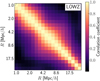Fig. 1 Correlation matrix estimate from jackknife resampling for the LOWZ measurement, using the full sample as shape tracers.

3.2 Covariance estimate

We estimated the covariance of $⟨N_{\mathrm{a}\mathrm{p}}{N}_{\mathrm{a}\mathrm{p}}{M}_{\mathrm{a}\mathrm{p}}^{\mathrm{I}}⟩$ directly from the data using jackknife resampling, both for the observed LOWZ and simulated MICE galaxies (see Sect. 4). For this, the survey was divided into 100 tiles with approximately the same area. We estimated ${\hat{G}}^{{\mathrm{\Pi }}_{\mathrm{m}}}$ for each of these tiles individually. We then combine the estimates for all but the k-th tile to form the k-th jackknife sample and converted it to the aperture statistics, which gave us 100 jackknife samples, we write as ${⟨N_{\mathrm{a}\mathrm{p}}{N}_{\mathrm{a}\mathrm{p}}{M}_{\mathrm{a}\mathrm{p}}^{\mathrm{I}}⟩}_k$. The i-j component of the covariance of $⟨N_{\mathrm{a}\mathrm{p}}{N}_{\mathrm{a}\mathrm{p}}{M}_{\mathrm{a}\mathrm{p}}^{\mathrm{I}}⟩$ is then $$\begin{array}{rl}{\hat{C}}_{ij}=& \frac{100}{100-1}\sum _{k=1}^{100}[⟨N_{\mathrm{a}\mathrm{p}}{N}_{\mathrm{a}\mathrm{p}}{M}_{\mathrm{a}\mathrm{p}}^{\mathrm{I}}{⟩}_k(R_i)-\overline{⟨N_{\mathrm{a}\mathrm{p}}{N}_{\mathrm{a}\mathrm{p}}{M}_{\mathrm{a}\mathrm{p}}^{\mathrm{I}}{⟩}_k}(R_i)]\\ & \times [⟨N_{\mathrm{a}\mathrm{p}}{N}_{\mathrm{a}\mathrm{p}}{M}_{\mathrm{a}\mathrm{p}}^{\mathrm{I}}{⟩}_k(R_j)-\overline{⟨N_{\mathrm{a}\mathrm{p}}{N}_{\mathrm{a}\mathrm{p}}{M}_{\mathrm{a}\mathrm{p}}^{\mathrm{I}}{⟩}_k}(R_j)],\end{array}$$(33)

where $\overline{{⟨N_{\mathrm{a}\mathrm{p}}{N}_{\mathrm{a}\mathrm{p}}{M}_{\mathrm{a}\mathrm{p}}^{\mathrm{I}}⟩}_k}\left({\theta }_i\right)$ is the average of all aperture statistics jackknife samples. We used ${\sigma }_i=\sqrt{{\hat{C}}_{ii}}$ as statistical uncertainty on the measured aperture statistics. To estimate the inverse covariance, we applied the Hartlap-correction (Hartlap et al. 2007), i.e., the estimate of the inverse covariance is the inverse of $\hat{C}$ multiplied by the factor $$\alpha =\frac{N-p-2}{N-1},$$(34)

where N = 100 is the number of samples and p is the number of entries in the data vector.

We show the correlation matrix, defined by ${\hat{C}}_{ij}/({\sigma }_i{\sigma }_j)$, for the LOWZ measurement in Fig. 1. The correlation matrix is dominated by the diagonal, suggesting that shape noise, in contrast to sample variance, is the biggest contributor. However, we see strong non-diagonal contributions. In particular, the signal for nearby scales is strongly correlated. This is expected for aperture statistics. They combine information from the correlation functions at different scales, which causes correlations between the aperture statistics at different aperture radii. The correlation matrix for $⟨N_{\mathrm{a}\mathrm{p}}{N}_{\mathrm{a}\mathrm{p}}{M}_{\mathrm{a}\mathrm{p}}^{\mathrm{I}}⟩$ is qualitatively similar to the correlation matrix for cosmic shear dominated ⟨N_apN_apM_ap⟩, shown in Fig. 10 of Linke et al. (2022).

3.3 Model fit

We fitted the NLA-inspired model defined in Eq. (25) and Eq. (28) to our measurements. For a fixed cosmology, this model includes the galaxy bias b and the IA amplitude A_IA as free parameters, but we fix the value of b from second-order statistic measurements. For the LOWZ galaxies, we use b = 1.77 determined by Singh et al. (2015) from second-order statistics. For the MICE galaxies, though, we use b = 1.47, which is 17% lower. We use this because the two-point galaxy correlation function in the MICE is approximately 30% lower than in the LOWZ, which suggests this lower galaxy bias value (Hoffmann et al. 2022).

Alternatively, one could also infer the galaxy bias and IA amplitude simultaneously from a third-order only analysis. For this, we would require additional measurements of either the position-shape-shape or position-position-position correlations. However, the position-shape-shape correlation has a low signal-to-noise in our sample and cannot be used for this exercise. We also opted against using the position-position-position correlation, even though it is detectable, since this correlation depends even more strongly on non-linear bias terms than the position-position-shape correlation: the relevant bispectrum includes terms proportional to b² b₂, not only b b. Consequently, our assumption of vanishing non-linear bias terms is likely inappropriate for this statistic, and we would need to include b₂ as an additional parameter in the model. Additionally, constraints on b from third-order statistics are weaker than those from second-order statistics. Therefore, we can constrain A_IA to a higher precision when using the b from second-order statistics. Consequently, we decided to use the simpler galaxy bias model and included the b from the second-order measurements.

Thus, the only free parameter remaining is A_IA, which we obtained by fitting the model to the measurements with a least-squares minimizer (Nelder & Mead 1965), including the covariance matrix obtained in Eq. (33). To investigate the model validity across different scales, we performed two fits for each measurement. One fit considers the aperture statistics for all scales R ∈ [1 h⁻¹ Mpc, 20 h⁻¹ Mpc]. This includes much smaller scales than the NLA model is considered valid for second-order statistics. We further conducted a second fit, where we limited the measurements to R > 6 h⁻¹ Mpc. This is the smallest scale considered by Singh et al. (2015) to be valid for the NLA model for second-order statistics. However, we note that the aperture radii R cannot be directly compared to the galaxy separation scale of the two-point correlation function, considered by Singh et al. (2015). Instead, aperture statistics for radius R include the correlation function both at smaller scales and (depending on the filter function) slightly larger scales than R.

4 Data

4.1 SDSS III BOSS LOWZ galaxies

Our primary dataset is the SDSS BOSS LOWZ galaxy sample, previously used by Singh & Mandelbaum (2016). This sample consists of luminous red galaxies (LRGs) at low redshifts, which were observed by DR8 of the SDSS (Aihara et al. 2011) and the BOSS DR11 (Alam et al. 2015). Shape measurements for these galaxies were carried out by Reyes et al. (2012). They reported galaxy ellipticities χ = (1 − q²)/(1 + q²), where q is the minor-to-major axis ratio q. However, the ellipticity in Eq. (1) is defined as ε = (1 − q)/(1 + q), so we converted χ to ε using the same relation as Singh & Mandelbaum (2016), $$ϵ=\frac{\chi }{2\mathcal{R}},$$(35)

where ℛ = 0.925.

The sample is constructed to contain a volume-limited sample of LRGs, so a selection in both redshift and colour-magnitude space was performed. The selection cuts were $$\begin{array}{lr}{m}_r<13.5+c_{\parallel }/0.3+\mathrm{\Delta }{m}_r& 16.0<m_r<19.6+\mathrm{\Delta }{m}_r\\ \left|c_{\perp }\right|<0.2& 0.16<z<0.36,\end{array}$$(36)

with $$\begin{array}{rl}& c_{\parallel }=0.7(m_g-m_r)+1.2[(m_r-m_i)-0.18]\\ & c_{\perp }=(m_r-m_i)-0.25(m_g-m_r)-0.18.\end{array}$$(37)

For the LOWZ galaxies, Δm_r = 0; however, for the simulated galaxies (see next section), Δm_r needs to be set to 0.085 to match the number density of the observed galaxies. We refer to Singh et al. (2015) for more details on the selection.

Following Singh et al. (2015), we further divided the galaxy sample into four luminosity bins L₁ − L₄ with L₁ containing the brightest galaxies. The bins L₁ − L₃ each contain 20% of the galaxies, with L₄ containing the remaining 40% faintest galaxies. In the following we consider correlations between the shapes of galaxies from one of these luminosity bins with the positions of the whole galaxy sample.

4.2 MICE with IA

To test our measurement pipeline, we used a catalogue of realistically simulated galaxies based on the MICE grand challenge light cone simulation (Fosalba et al. 2015a). MICE is a dark-matter only N-body simulation that adopts a flat ΛCDM cosmology with parameters Ω_m = 0.25, Ω_Λ = 0.75, Ω_b = 0.044, n_s = 0.95, σ₈ = 0.8, h = 0.7. The simulation tracks the evolution of 4096³ particles, each with a mass of 2.93 × 10¹⁰ h⁻¹ M_⊙, within a cubic volume of side length 3072h⁻¹ Mpc, spanning from an initial redshift of z = 100 to the present time. Halos were identified with a Friends-of-friends halo finder (Crocce et al. 2015). Subsequently, the halos were populated with galaxies up to redshift z = 1.4, using a combination of halo abundance matching and a halo occupation distribution model (Carretero et al. 2015). The galaxies received positions, luminosities and colours such that their luminosity function and colour-magnitude distribution matched SDSS observations (Blanton et al. 2003; Zehavi et al. 2011).

The MICE was initially designed to accompany gravitational lensing surveys, so an estimate of each galaxy’s weak lensing shear was computed by projecting the mass distribution and applying the Born approximation as described in Fosalba et al. (2015b, 2008). Hoffmann et al. (2022) added realistic intrinsic galaxy ellipticites using a semi-analytic IA model. In this procedure, the simulated galaxies are divided into red and blue central galaxies and satellites; red centrals receive a 3D orientation aligned with their host halo, while blue centrals are aligned with the angular momentum of their host halo. Satellites are assumed to point towards their host halo centre. These orientations are then distorted by a randomly assigned misalignment angle. The distribution of misalignment angles depends on galaxy colour and magnitude. It is calibrated such that the simulated galaxies reproduce the second-order correlation between intrinsic shapes and galaxy positions observed in the LOWZ galaxy sample as well as the observed distribution of galaxy axis ratios from COSMOS (Laigle et al. 2016; Griffith et al. 2012). Simulated galaxy positions, shapes, and other properties for an octant on the sky are available via Cosmohub³ (Tallada et al. 2020; Carretero et al. 2017).

From the MICE with IA, we selected a sample mimicking the LOWZ galaxies on the provided sky octant (5156.6 deg², so approximately half the BOSS footprint). We applied the same selection as in Eq. (36). However, similar to Hoffmann et al. (2022), we set Δm_r to 0.085 to match the number density of the LOWZ galaxies. As with the LOWZ sample, we divided the simulated galaxies into four luminosity bins, containing 20, 20, 20 and 40% of the galaxy sample, respectively. We used only the intrinsic galaxy shapes and neglected the cosmic shear contribution. We also used the ‘true’ (or purely cosmological) redshifts of the sample; that is, we neglected any impact of redshift space distortions.

5 Results

As mentioned in Sect. 3.3, we fitted the NLA-inspired model to our measurements firstly using all aperture radii and then restricted to scales above 6 h⁻¹ Mpc, with galaxy bias values obtained by Singh et al. (2015). The resulting values for A_IA are listed in Table 1 and the reduced χ² values in Table 2. In Fig. 2, we show the A_IA for the larger-scale fits as a function of the mean absolute magnitude M_r of the samples.

For all luminosity bins, A_IA is significantly non-zero. Using the large-scale (all-scale) fit, A_IA for the full LOWZ sample is 4.7σ (7.6σ) larger than zero. The strongest detection occurs for the brightest sample with 5.9σ for the large-scale fit. As expected, A_IA is largest for the brightest galaxies, which are expected to show the strongest alignment, and decreases for fainter galaxies.

Also shown in Fig. 2, and listed in Table 1, are the values for A_IA estimated by Singh et al. (2015) from second-order correlations. Our third-order based estimates are consistent with these second-order based estimates within their 1σ uncertainties for all luminosity bins. As we are considering the same sample for the second and third-order measurements, the sample variance contributions to the uncertainties of the two cases are correlated. Therefore, we expect a deviation of less than the 1σ uncertainties. The other contributions to the uncertainties, namely the source galaxies’ shape noise and the shot noise of the lens galaxy distribution, contribute differently to the second and third-order measurements and are thus less correlated.

Figure 2 also shows the A_IA obtained from fitting the model to the measurements for the simulated MICE galaxies. Their A_IA show the same trends as for the observed galaxies and agree with them within 1–2σ. Generally, A_IA is lower in the simulation than observed, except for the faintest galaxies in the L4 sample. However, the MICE galaxies have slightly different mean luminosities and luminosity distributions, so slight differences are not unexpected.

Table 1 shows that we obtain smaller values for A_IA when fitting to all measured scales than when considering only larger scales. To understand this, we show the measurement and both fits for the full sample in Fig. 3 and the individual luminosity bins in Fig. 4. For all LOWZ galaxy samples the signal flattens at small scales. This flattening cannot be described by our simple model that only contains a scale-independent parameter. The fit compensates for this inadequacy by lowering A_IA across all scales.

As can be seen in Table 2, including the small scales leads to overall worse fits with larger χ² values. This confirms that the model cannot accurately describe the small scales. Moreover, the difference between the inferred A_IA and the estimate from second-order statistics is greater when including the small scales. For the L1 and L3 galaxies, the estimates no longer agree within the 1σ uncertainty, so the extrapolation of the third-order model to small scales is not consistent with the second-order model at larger scales.

The MICE galaxies show the same trends as the LOWZ galaxies. Aside from the L2 sample, we see the same flattening of the signal at small scales. For the brightest galaxies, we also find a more than 1σ difference in the A_IA inferred from the fit to the whole scale range compared to the second-order estimate.

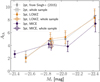Fig. 2 IA amplitude AIA as a function of the mean absolute magnitude Mr of the shape tracers for the LOWZ galaxies (pink circles) and for the MICE (green diamonds) as obtained from the third-order IA measurement at scales R > 6 h−1 Mpc. Also shown are the estimates by Singh et al. (2015) from second-order statistics (black squares). Open symbols are the estimates for the whole shape tracing sample.

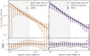Fig. 3 Comparison of IA measurements for full LOWZ and simulated galaxy samples to model fits. Upper panels: IAaperture statistics for full galaxy samples. The left panel shows the measurements for the LOWZ galaxies; the right panel shows measurements for the simulated MICE galaxies. Points are measurements with jackknife error estimates. Solid lines show the model fit using scales above 6 h−1 Mpc; dashed lines are the model fit using all shown scales. Lower panels: relative difference of measurement to model fit for large scales.

6 Discussion

We presented the first detection of a third-order intrinsic alignment (IA) correlation in the Sloan Digital Sky Survey (SDSS) Baryon Oscillation Spectroscopic Survey (BOSS) LOWZ galaxies. For this, we measured the third-order correlation function between galaxy positions and shapes and expressed them in terms of aperture statistics. We compared the measured signal with predictions by the Marenostrum Institut de Ciències de l’Espai (MICE) cosmological simulation and a non-linear linear alignment (NLA) based analytical model. Our measurements depend on the B_δδI contribution to the bispectrum of matter densities and galaxy shapes, the matter-matter-shape correlation. The positions of the LOWZ galaxies are used as tracers for the matter distribution, which were then correlated with their shapes.

We find a significant third-order IA signal. For scales between 6 h⁻¹ Mpc and 20 h⁻¹ Mpc and using the full LOWZ galaxy sample, we find an IA amplitude A_IA = 4.4 ± 0.93, which is a non-zero signal at 4.7σ. After dividing the sample into subsamples based on galaxy luminosity, we find an increased S/N for the brightest galaxies while the S/N for the fainter galaxies decreases. However, even for the faintest galaxies, A_IA is still non-zero at 3.6σ. This dependence of the signal on the galaxy luminosity is not surprising, as IA has been shown to increase with galaxy luminosity and stellar mass, both in observations (Singh et al. 2015; Singh & Mandelbaum 2016; Johnston et al. 2019) and hydrodynamical simulations (Samuroff et al. 2021).

Comparing the measurements from the observations to the predictions by the MICE simulation, we again find that the bestfitting A_IA increases with luminosity. Indeed, the A_IA s from the simulation agree with the LOWZ measurements at 1–2σ. At first glance, this agreement might seem unsurprising as the intrinsic shapes of the simulated galaxies have been tuned to reproduce the second-order IA measurements by Singh et al. (2015) in the LOWZ sample. Moreover, the third-order galaxy clustering of MICE galaxies has been successfully validated (Hoffmann et al. 2015). However, the agreement is a crucial consistency check for two reasons. First, the agreement suggests that tuning the simulation to the second-order statistics automatically provides the correct third-order statistics, lending credibility to the physical model implemented in the simulation. Second, only the intrinsic galaxy shapes were used for the simulation measurements without adding cosmic shear. Consequently, the agreement of the measurements in the observations, where we cannot turn off cosmic shear, shows that weak lensing does not significantly bias our measurement. This validates our choice of Π_m, the maximal distance between galaxies in a triplet considered for the correlation function measurement. Evidently, the chosen Π_m is small enough that cosmic shear correlations become sub-dominant.

Finally, we compared the A_IA from the model fits to the third-order IA signal to the estimates by Singh et al. (2015) from second-order statistics. The A_IA obtained from fitting to scales above 6 h⁻¹ Mpc agree within 1σ with the second-order estimates. Consequently, at these scales, the second and third-order models are consistent and can be used in a combined analysis. This combination offers the opportunity for IA self-calibration (Pyne & Joachimi 2021), leading to tighter constraints on both IA and cosmological parameters.

The A_IA values inferred from the fit, including smaller scales, agree less well with the second-order based estimates. While the agreement is still within 2σ for all luminosity samples, the measurements show a flattening at small scales that cannot be described with our simple NLA-inspired model. Furthermore, the goodness-of-fit, as indicated by the reduced χ² values, degrades when small scales are included. This shows that the model is no longer accurate at small scales. There are several possible reasons for this inaccuracy, among them the inaccuracy of the NLA approach, non-linear contributions to the galaxy bias, and small-scale physical effects such as baryonic feedback. Regarding the NLA model, Singh et al. (2015) find that the NLA model cannot well describe the second-order IA statistics for scales below 6 h⁻¹ Mpc. Thus, it seems natural that the NLA-inspired model also breaks down at small scales. As mentioned before, the NLA model is an effective, phenomenological description of IA and is not rigorously physically motivated. Higher-order corrections thus become necessary for small scales.

Another consideration in explaining the model deviations is our choice of a simple linear deterministic galaxy bias. In a perturbation theory approach, the galaxy bispectrum already depends on the non-linear galaxy bias at the leading order. We showed that a non-zero b₂, which is the first non-linear bias term, only has a small impact on the model compared to the measurement uncertainties and thus can be neglected for the sample and scales we consider here. Higher order contributions, i.e., b₃, b₄, and so on, enter at most at the next-to-leading order, so they likely have even less impact on the model. Thus, it seems unlikely that the full ‘flattening’ of the signal can be explained by non-linear galaxy bias terms. However, galaxy bias depends strongly on the selected sample, so while we could simplify our model by neglecting non-linear galaxy bias, this simplification might not be appropriate for different sample choices. We also neglected the quadratic non-local bias, which depends on the tidal field.

Small-scale physics, such as baryonic feedback, could also be part of the cause of the model breakdown at small scales. Baryonic feedback leads to a suppression of the matter power and bispectrum at small scales. This would also suppress the third-order IA signal for small aperture radii. However, the concrete values for the bispectrum suppression are unclear, with predictions from hydrodynamical simulations ranging between less than 1 and 20% at k = 1 h Mpc⁻¹, while in some simulations there is even an enhancement of the bispectrum at k ≃ 3 h Mpc⁻¹ (see e.g. Aricò et al. 2021; Foreman et al. 2020).

The perturbation theory approach itself becomes inaccurate when entering the regime of single dark matter halos, so a more sophisticated third-order IA model might be needed at small scales. For example, the bispectrum B_ggI could be modelled by using a halo model approach for the correlation between galaxies and matter (Linke et al. 2022), multiplied by the NLA prefactor f₁. Alternatively, a full halo model for the IA signal might be devised in the spirit of Fortuna et al. (2021). However, in light of the general good agreement, we see no necessity to use a more complex IA model to describe the LOWZ data set. This might change for other surveys with more constraining power, for example, those expected by Euclid, LSST, and DESI. Repeating our measurements on a more extensive survey and other galaxy samples can help decide whether the NLA-inspired model is still appropriate for analysing third-order statistics in upcoming stage-IV surveys. Additionally, other third-order statistics, for example, shape-shape-lens correlations or the related bispectra, could be explored to further test the model’s consistency.

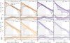Fig. 4 Same as Fig. 3, but for the different luminosity samples, with L1 containing the brightest and L4 the faintest galaxies.

Acknowledgements

We thank the anonymous referee for their helpful comments. The authors acknowledge the support of the Lorentz Center and the echoIA project. L.L. is supported by the Austrian Science Fund (FWF) [ESP 357-N]. S.P. and B.J. acknowledge support by the ERC-selected UKRI Frontier Research Grant EP/Y03015X/1. S.P. acknowledges the Lendület Program of the Hungarian Academy of Sciences and hospitality from MTA-CSFK Lendület “Momentum” Large-Scale Structure Research Group, Konkoly Observatory, Budapest. This publication is part of the project “A rising tide: Galaxy intrinsic alignments as a new probe of cosmology and galaxy evolution” (with project number VI.Vidi.203.011) of the Talent programme Vidi which is (partly) financed by the Dutch Research Council (NWO). R.M. acknowledges the support of the Simons Foundation (Simons Investigator in Astrophysics, Award ID 620789). This work has made use of CosmoHub. CosmoHub has been developed by the Port d’Informació Científica (PIC), maintained through a collaboration of the Institut de Física d’Altes Energies (IFAE) and the Centro de Investigaciones Energéticas Medioambientales y Tecnológicas (CIEMAT) and the Institute of Space Sciences (CSIC & IEEC). CosmoHub was partially funded by the “Plan Estatal de Investigación Científica y Técnica de Innovación” program of the Spanish government, has been supported by the call for grants for Scientific and Technical Equipment 2021 of the State Program for Knowledge Generation and Scientific and Technological Strengthening of the R+D+i System, financed by MCIN/AEI/ 10.13039/501100011033 and the EU NextGeneration/PRTR (Hadoop Cluster for the comprehensive management of massive scientific data, reference EQC2021-007479-P) and by MICIIN with funding from European Union NextGenerationEU(PRTR-C17.I1) and by Generalitat de Catalunya. Funding for SDSS-III has been provided by the Alfred P. Sloan Foundation, the Participating Institutions, the National Science Foundation, and the U.S. Department of Energy Office of Science. The SDSS-III website is http://www.sdss3.org. SDSS-III is managed by the Astrophysical Research Consortium for the Participating Institutions of the SDSS-III Collaboration including the University of Arizona, the Brazilian Participation Group, Brookhaven National Laboratory, Carnegie Mellon University, University of Florida, the French Participation Group, the German Participation Group, Harvard University, the Instituto de Astrofisica de Canarias, the Michigan State/Notre Dame/JINA Participation Group, Johns Hopkins University, Lawrence Berkeley National Laboratory, Max Planck Institute for Astrophysics, Max Planck Institute for Extraterrestrial Physics, New Mexico State University, New York University, Ohio State University, Pennsylvania State University, University of Portsmouth, Princeton University, the Spanish Participation Group, University of Tokyo, University of Utah, Vanderbilt University, University of Virginia, University of Washington, and Yale University.

Appendix A Relation of aperture statistics to bispectrum

To model $⟨N_{\mathrm{a}\mathrm{p}}{N}_{\mathrm{a}\mathrm{p}}{M}_{\mathrm{a}\mathrm{p}}^{\mathrm{I}}⟩$, we relate it to the galaxy-galaxy-shape bispectrum B_ggI. For this, we first write it as $$\begin{array}{rl}⟨N_{\mathrm{a}\mathrm{p}}{N}_{\mathrm{a}\mathrm{p}}{M}_{\mathrm{a}\mathrm{p}}^{\mathrm{I}}⟩(R_1,R_2,R_3)=& \int \mathrm{d}\chi p(\chi )\int \mathrm{d}{\chi }_{1}p\left({\chi }_1\right)\int \mathrm{d}{\chi }_{2}p\left({\chi }_2\right)\int {\mathrm{d}}^2{r}_1^{\mathrm{\prime }}\int {\mathrm{d}}^2{r}_2^{\mathrm{\prime }}\int {\mathrm{d}}^2{r}_3^{\mathrm{\prime }}{U}_R\left(r_1^{\mathrm{\prime }}\right)U_R\left(r_2^{\mathrm{\prime }}\right)U_R\left(r_3^{\mathrm{\prime }}\right)\\ & \times ⟨{\delta }_{\mathrm{g}}(\mathit{r}-{\mathit{r}}_1,{\chi }_1){\delta }_{\mathrm{g}}(\mathit{r}-{\mathit{r}}_2,{\chi }_2){\delta }_{\mathrm{I}}(\mathit{r}-{\mathit{r}}_3,\chi )⟩.\end{array}$$(A.1)

We now use the galaxy-galaxy-intrinsic shape bispectrum B_ggI defined by $$(2\pi {)}^3{\delta }_{\mathrm{D}}({\mathit{k}}_1+{\mathit{k}}_2+{\mathit{k}}_3)B_{\mathrm{g}\mathrm{g}\mathrm{I}}(k_1,k_2,k_3;{\chi }_1,{\chi }_2,\chi )=⟨\widetilde{{\delta }_{\mathrm{g}}}({\mathit{k}}_1,{\chi }_1)\widetilde{{\delta }_{\mathrm{g}}}({\mathit{k}}_2,{\chi }_2)\widetilde{{\delta }_{\mathrm{I}}}({\mathit{k}}_3,\chi )⟩,$$(A.2)

and separate the k_i into their components k_z,i along the line-of-sight and k_⊥,i perpendicular to the line-of-sight. With this, $$\begin{array}{rl}⟨N_{\text{ap }}{N}_{\text{ap }}{M}_{\text{ap }}^{\mathrm{I}}⟩(R_1,R_2,R_3)=& \int \mathrm{d}\chi p(\chi )\int \mathrm{d}{\chi }_{1}p({\chi }_1)\int \mathrm{d}{\chi }_{2}p({\chi }_2)\int \frac{{\mathrm{d}}^2{k}_{\perp ,1}}{(2\pi {)}^2}\int \frac{{\mathrm{d}}^2{k}_{\perp ,2}}{(2\pi {)}^2}\int \frac{{\mathrm{d}}^2{k}_{\perp ,3}}{(2\pi {)}^2}{\tilde{U}}_R(k_{\perp ,1}){\tilde{U}}_R(k_{\perp ,2}){\tilde{U}}_R(k_{\perp ,3})\\ & \times \int \frac{\mathrm{d}{k}_{z,1}}{2\pi }\int \frac{\mathrm{d}{k}_{z,2}}{2\pi }\int \frac{\mathrm{d}{k}_{z,3}}{2\pi }{\mathrm{e}}^{-\mathrm{i}(k_{z,1}\chi 1+k_{z2}\chi 2+k_{z,3}\chi .}(2\pi {)}^3{\delta }_{\mathrm{D}}(k_1+{\mathit{k}}_2+{\mathit{k}}_3)B_{\mathrm{g}\mathrm{g}\mathrm{I}}(k_1,k_2,k_3;{\chi }_1,{\chi }_2,\chi ).\end{array}$$(A.3)

Evaluating the k₃ integrals leads to $$\begin{array}{rl}⟨N_{\mathrm{a}\mathrm{p}}{N}_{\mathrm{a}\mathrm{p}}{M}_{\mathrm{a}\mathrm{p}}^{\mathrm{I}}⟩(R_1,R_2,R_3)=& \int \mathrm{d}\chi p(\chi )\int \mathrm{d}{\chi }_{1}p({\chi }_1)\int \mathrm{d}{\chi }_{2}p({\chi }_2)\int \frac{{\mathrm{d}}^2{k}_{\perp ,1}}{(2\pi {)}^2}\int \frac{{\mathrm{d}}^2{k}_{\perp ,2}}{(2\pi {)}^2}{\tilde{U}}_R(k_{\perp ,1}){\tilde{U}}_R(k_{\perp ,2}){\tilde{U}}_R(\mid k_{\perp ,1}+k_{\perp ,2}\mid )\\ & \times \int \frac{\mathrm{d}{k}_{z,1}}{2\pi }\int \frac{\mathrm{d}{k}_{z,2}}{2\pi }{\mathrm{e}}^{-\mathrm{i}{k}_{z,1}({\chi }_1-\chi )+\mathrm{i}{k}_{z,2}({\chi }_2-\chi )}{B}_{\mathrm{g}\mathrm{g}\mathrm{I}}(k_1,k_2,k_3;{\chi }_1,{\chi }_2,\chi ).\end{array}$$(A.4)

Now, we use the Limber approximation, under which $$B_{\mathrm{g}\mathrm{g}\mathrm{I}}(k_1,k_2,k_3;{\chi }_1,{\chi }_2,\chi )\simeq B_{\mathrm{g}\mathrm{g}\mathrm{I}}(k_{\perp ,1},k_{\perp ,2},k_{\perp ,3};{\chi }_1,{\chi }_2,\chi ).$$(A.5)

Inserting this, evaluating the k_z,i integrals and the (then trivial) χ₁ and χ₂ integrals leads to $$⟨N_{\text{ap }}{N}_{\text{ap }}{M}_{\text{ap }}^{\mathrm{I}}⟩(R_1,R_2,R_3)=\int \frac{{\mathrm{d}}^2{k}_{\perp ,1}}{(2\pi {)}^2}\int \frac{{\mathrm{d}}^2{k}_{\perp ,2}}{(2\pi {)}^2}{\tilde{U}}_R(k_{\perp ,1}){\tilde{U}}_R(k_{\perp ,2}){\tilde{U}}_R(\mid k_{\perp ,1}+k_{\perp ,2}\mid )\int \mathrm{d}\chi p^3(\chi )B_{\mathrm{g}\mathrm{g}\mathrm{I}}(k_{\perp ,1},k_{\perp ,2},k_{\perp ,3};\chi ,\chi ,\chi ),$$(A.6)

so $⟨N_{\mathrm{a}\mathrm{p}}{N}_{\mathrm{a}\mathrm{p}}{M}_{\mathrm{a}\mathrm{p}}^{\mathrm{I}}⟩$ can be readily computed for a given filter function U, a galaxy redshift distribution p and a bispectrum model B_ggI.

Appendix B Impact of non-linear galaxy bias

As described in Eq. (28), the galaxy-matter bispectrum already depends on the non-linear galaxy bias b₂ at the leading order. However, we argue that b₂ can be neglected for the $⟨N_{\mathrm{a}\mathrm{p}}{N}_{\mathrm{a}\mathrm{p}}{M}_{\mathrm{a}\mathrm{p}}^{\mathrm{I}}⟩$ modelling at the level of uncertainty of the LOWZ measurements. To demonstrate this, Fig. B.1 shows the best-fitting model for the LOWZ measurements in the full sample when neglecting b₂ and the model for the same A_IA and b but now setting b₂ = 1. For this, we computed the non-linear power spectrum using the revised halofit prescription (Takahashi et al. 2012).

When including a positive b₂, the model increases, particularly at larger scales, by up to 20%. However, this increase is small compared to the measurement uncertainty and both models show good agreement with the measurement. Therefore, the value of b₂ is not critical to describe the $⟨N_{\mathrm{a}\mathrm{p}}{N}_{\mathrm{a}\mathrm{p}}{M}_{\mathrm{a}\mathrm{p}}^{\mathrm{I}}⟩$ from the LOWZ.

We note that Fig B.1 depicts a pessimistic case, as we do not expect b₂ to be as large as one. Measurements of the bispectrum of galaxies from the LOWZ sample by Gil-Marín et al. (2017) find b₂ σ₈ = 0.6, which for σ₈ = 0.8 yields b₂ = 0.75. Using LOWZ-like simulated mock galaxies, Eggemeier et al. (2021) found the even lower value of b₂ = 0.3 ± 0.2. Consequently, the impact of the non-linear galaxy bias is likely even smaller than shown here.

Appendix C Estimator bias

The estimator for the correlation function in Eq. (30) is biased. To see this, we calculate the expectation value of the estimator. The expectation value of the numerator is $$⟨{\displaystyle \sum _{i=1}^{N_{\mathrm{L}}}}{\displaystyle \sum _{j=1}^{N_{\mathrm{L}}}}{\displaystyle \sum _{k=1}^{N_{\mathrm{S}}}}{ϵ}_k{\mathrm{e}}^{\mathrm{i}({\varphi }_i+{\varphi }_j)}\mathrm{\Delta }(r_1,r_2,\varphi ,{\mathit{x}}_i,{\mathit{x}}_j,{\mathit{x}}_k){\mathrm{\Theta }}_{{\mathrm{\Pi }}_{\mathrm{m}}}({\chi }_i,{\chi }_j;{\chi }_k)⟩$$(C.1) $$=\int {\mathrm{d}}^2{x}_1\int {\mathrm{d}}^2{x}_2\int {\mathrm{d}}^2{x}_3\int \mathrm{d}{\chi }_1\int \mathrm{d}{\chi }_2\int \mathrm{d}{\chi }_{3}p({\chi }_1)p({\chi }_2)p({\chi }_3)⟨n({\mathit{x}}_1,{\chi }_1)n({\mathit{x}}_2,{\chi }_2)ϵ({\mathit{x}}_3,{\chi }_3){\mathrm{e}}^{-\mathrm{i}({\varphi }_1+{\varphi }_2)}⟩$$(C.2)

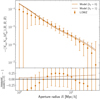Fig. B.1 Comparison of IA measurements for LOWZ sample with and without non-linear bias. Upper panel: Measurement of $⟨N_{\mathrm{a}\mathrm{p}}{N}_{\mathrm{a}\mathrm{p}}{M}_{\mathrm{a}\mathrm{p}}^{\mathrm{I}}⟩$ for full LOWZ sample (points), with model fit without non-linear bias (solid line) and same model but using b2 = 1 (dashed line). Lower panel: Relative difference to the model, which neglects non-linear bias.

$$\begin{array}{rl}& \times \mathrm{\Delta }(r_1,r_2,\varphi ,{\mathit{x}}_1,{\mathit{x}}_2,{\mathit{x}}_3){\mathrm{\Theta }}_{{\mathrm{\Pi }}_{\mathrm{m}}}({\chi }_1,{\chi }_2;{\chi }_3)\\ =& \int \mathrm{d}\chi {\int }_{{\chi }_{}-{\mathrm{\Pi }}_{\mathrm{m}}}^{{\chi }_{\mathrm{m}}+{\mathrm{\Pi }}_{\mathrm{m}}}\mathrm{d}{\chi }_1{\int }_{\chi -{\mathrm{\Pi }}_{\mathrm{m}}}^{\chi +{\mathrm{\Pi }}_{\mathrm{m}}}\mathrm{d}{\chi }_{2}p({\chi }_1)p({\chi }_2)p(\chi )⟨n({\mathit{x}}_3+{\mathit{r}}_1,{\chi }_1)n({\mathit{x}}_3+{\mathit{r}}_2,{\chi }_2)ϵ({\mathit{x}}_3,\chi ){\mathrm{e}}^{-\mathrm{i}({\varphi }_1+{\varphi }_2)}⟩\\ =& {\overline{N}}_{{\mathrm{\Pi }}_{\mathrm{m}}}^2{G}^{{\mathrm{\Pi }}_{\mathrm{m}}}({\mathit{r}}_1,{\mathit{r}}_2).\end{array}$$(C.3)

The expectation value of the denominator is $$⟨{\displaystyle \sum _{i=1}^{N_{\mathrm{L}}}}{\displaystyle \sum _{j=1}^{N_{\mathrm{L}}}}{\displaystyle \sum _{k=1}^{N_{\mathrm{S}}}}\mathrm{\Delta }(r_1,r_2,\varphi ,{\mathit{x}}_i,{\mathit{x}}_j,{\mathit{x}}_k){\mathrm{\Theta }}_{{\mathrm{\Pi }}_{\mathrm{m}}}({\chi }_i,{\chi }_j;{\chi }_k)⟩$$(C.4) $$=\int {\mathrm{d}}^2{x}_1\int {\mathrm{d}}^2{x}_2\int {\mathrm{d}}^2{x}_3\int \mathrm{d}{\chi }_1\int \mathrm{d}{\chi }_2\int \mathrm{d}{\chi }_{3}p({\chi }_1)p({\chi }_2)p({\chi }_3)⟨n({\mathit{x}}_1,{\chi }_1)n({\mathit{x}}_2,{\chi }_2)⟩\mathrm{\Delta }(r_1,r_2,\varphi ,{\mathit{x}}_1,{\mathit{x}}_2,{\mathit{x}}_3){\mathrm{\Theta }}_{{\mathrm{\Pi }}_{\mathrm{m}}}({\chi }_1,{\chi }_2,{\chi }_3)$$(C.5) $$=\int \mathrm{d}\chi {\int }_{\chi -{\mathrm{\Pi }}_{\mathrm{m}}}^{\chi +{\mathrm{\Pi }}_{\mathrm{m}}}\mathrm{d}{\chi }_1{\int }_{\chi -{\mathrm{\Pi }}_{\mathrm{m}}}^{\chi +{\mathrm{\Pi }}_{\mathrm{m}}}\mathrm{d}{\chi }_{2}p({\chi }_1)p({\chi }_2)p(\chi )⟨n({\mathit{x}}_3+{\mathit{r}}_1,{\chi }_1)n({\mathit{x}}_3+{\mathit{r}}_2,{\chi }_2)⟩$$(C.6) $$=\int \mathrm{d}\chi {\int }_{\chi -{\mathrm{\Pi }}_{\mathrm{m}}}^{\chi +{\mathrm{\Pi }}_{\mathrm{m}}}\mathrm{d}{\chi }_1{\int }_{\chi -{\mathrm{\Pi }}_{\mathrm{m}}}^{\chi +{\mathrm{\Pi }}_{\mathrm{m}}}\mathrm{d}{\chi }_{2}p({\chi }_1)p({\chi }_2)p(\chi )\times \overline{n}({\chi }_1)\overline{n}({\chi }_2)[1+\xi (|{\mathit{r}}_1-{\mathit{r}}_2|,|{\chi }_1-{\chi }_2\mid )].$$(C.7)

Here, ξ(Δr, Δχ) is the three-dimensional galaxy clustering function for galaxy pairs separated by Δr in projection and by Δχ along the line-of-sight. This expectation value can be approximated by $$\begin{array}{rl}& \int \mathrm{d}\chi {\int }_{\chi -{\mathrm{\Pi }}_{\mathrm{m}}}^{\chi +{\mathrm{\Pi }}_{\mathrm{m}}}\mathrm{d}{\chi }_1{\int }_{\chi -{\mathrm{\Pi }}_{\mathrm{m}}}^{\chi +{\mathrm{\Pi }}_{\mathrm{m}}}\mathrm{d}{\chi }_{2}p({\chi }_1)p({\chi }_2)p(\chi )\overline{n}({\chi }_1)\overline{n}({\chi }_2)[1+\xi (|{\mathit{r}}_1-{\mathit{r}}_2|,\mid {\chi }_1-{\chi }_2\mid )]\\ & \simeq {\overline{N}}_{{\mathrm{\Pi }}_{\mathrm{m}}}^2\int \mathrm{d}\chi {\int }_{\chi -{\mathrm{\Pi }}_{\mathrm{m}}}^{\chi +{\mathrm{\Pi }}_{\mathrm{m}}}\mathrm{d}{\chi }_1{\int }_{\chi -{\mathrm{\Pi }}_{\mathrm{m}}}^{\chi +{\mathrm{\Pi }}_{\mathrm{m}}}\mathrm{d}{\chi }_{2}p({\chi }_1)p({\chi }_2)p(\chi )[1+\xi (|{\mathit{r}}_1-{\mathit{r}}_2|,|{\chi }_1-{\chi }_2|)]\\ & ={\overline{N}}_{{\mathrm{\Pi }}_{\mathrm{m}}}^{2}B({\mathit{r}}_1,{\mathit{r}}_2,{\mathrm{\Pi }}_{\mathrm{m}}).\end{array}$$(C.8)

Therefore, the expectation value of the estimator ${\hat{G}}_{\text{bias }}^{{\mathrm{\Pi }}_m}$ is $$⟨{\hat{G}}_{\text{bias }}^{{\mathrm{\Pi }}_{\mathrm{m}}}⟩\simeq \frac{G^{{\mathrm{\Pi }}_{\mathrm{m}}}}{B({\mathit{r}}_1,{\mathit{r}}_2,{\mathrm{\Pi }}_{\mathrm{m}})}.$$(C.9)

We show in Fig. C.1 the B estimated for the full LOWZ sample. The bias is strongly scale-dependent.

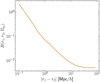Fig. C.1 Estimator bias B for the full LOWZ galaxy sample.

References

- Abbott, T., Abdalla, F. B., Allam, S., et al. 2016, Phys. Rev. D, 94, 022001 [Google Scholar]
- Aihara, H., Allende Prieto, C., An, D., et al. 2011, ApJS, 193, 29 [NASA ADS] [CrossRef] [Google Scholar]
- Aihara, H., Arimoto, N., Armstrong, R., et al. 2018, PASJ, 70, S4 [NASA ADS] [Google Scholar]
- Akeson, R., Armus, L., Bachelet, E., et al. 2019, arXiv e-prints [arXiv:1902.05569] [Google Scholar]
- Alam, S., Albareti, F. D., Allende Prieto, C., et al. 2015, ApJS, 219, 12 [Google Scholar]
- Amon, A., Gruen, D., Troxel, M. A., et al. 2022, Phys. Rev. D, 105, 023514 [NASA ADS] [CrossRef] [Google Scholar]
- Aricò, G., Angulo, R. E., Hernández-Monteagudo, C., Contreras, S., & Zennaro, M. 2021, MNRAS, 503, 3596 [Google Scholar]
- Asgari, M., Lin, C.-A., Joachimi, B., et al. 2021, A&A, 645, A104 [NASA ADS] [CrossRef] [EDP Sciences] [Google Scholar]
- Bartelmann, M., & Schneider, P. 2001, Phys. Rep., 340, 291 [Google Scholar]
- Becker, M. R., Troxel, M. A., MacCrann, N., et al. 2016, Phys. Rev. D, 94, 022002 [NASA ADS] [CrossRef] [Google Scholar]
- Blanton, M. R., Hogg, D. W., Bahcall, N. A., et al. 2003, ApJ, 592, 819 [Google Scholar]
- Blazek, J. A., MacCrann, N., Troxel, M. A., & Fang, X. 2019, Phys. Rev. D, 100, 103506 [NASA ADS] [CrossRef] [Google Scholar]
- Bridle, S., & King, L. 2007, New J. Phys., 9, 444 [Google Scholar]
- Burger, P. A., Porth, L., Heydenreich, S., et al. 2024, A&A, 683, A103 [NASA ADS] [CrossRef] [EDP Sciences] [Google Scholar]
- Carretero, J., Castander, F. J., Gaztañaga, E., Crocce, M., & Fosalba, P. 2015, MNRAS, 447, 646 [NASA ADS] [CrossRef] [Google Scholar]
- Carretero, J., Tallada, P., Casals, J., et al. 2017, in Proceedings of the European Physical Society Conference on High Energy Physics. 5-12 July, 488 [CrossRef] [Google Scholar]
- Catelan, P., Kamionkowski, M., & Blandford, R. D. 2001, MNRAS, 320, L7 [NASA ADS] [CrossRef] [Google Scholar]
- Chen, S.-F., & Kokron, N. 2024, J. Cosmology Astropart. Phys., 1, 027 [CrossRef] [Google Scholar]
- Crittenden, R. G., Natarajan, P., Pen, U.-L., & Theuns, T. 2002, ApJ, 568, 20 [NASA ADS] [CrossRef] [Google Scholar]
- Crocce, M., Castander, F. J., Gaztañaga, E., Fosalba, P., & Carretero, J. 2015, MNRAS, 453, 1513 [NASA ADS] [CrossRef] [Google Scholar]
- Dalal, R., Li, X., Nicola, A., et al. 2023, Phys. Rev. D, 108, 123519 [CrossRef] [Google Scholar]
- DES and KiDS Collaboration, Abbott, T. M. C., et al.) 2023, Open J. Astrophys., 6, 36 [NASA ADS] [Google Scholar]
- Eggemeier, A., Scoccimarro, R., Smith, R. E., et al. 2021, Phys. Rev. D, 103, 123550 [NASA ADS] [CrossRef] [Google Scholar]
- Eisenstein, D. J., & Hu, W. 1999, ApJ, 511, 5 [Google Scholar]
- Euclid Collaboration (Blanchard, A., et al.) 2020, A&A, 642, A191 [NASA ADS] [CrossRef] [EDP Sciences] [Google Scholar]
- Euclid Collaboration (Ajani, V., et al.) 2023, A&A, 675, A120 [NASA ADS] [CrossRef] [EDP Sciences] [Google Scholar]
- Euclid Collaboration (Mellier, Y., et al.) 2024, A&A, in press, https://doi.org/10.1051/0004-6361/202450810 [Google Scholar]
- Foreman, S., Coulton, W., Villaescusa-Navarro, F., & Barreira, A. 2020, MNRAS, 498, 2887 [NASA ADS] [CrossRef] [Google Scholar]
- Fortuna, M. C., Hoekstra, H., Johnston, H., et al. 2021, A&A, 654, A76 [NASA ADS] [CrossRef] [EDP Sciences] [Google Scholar]
- Fosalba, P., Gaztañaga, E., Castander, F. J., & Manera, M. 2008, MNRAS, 391, 435 [NASA ADS] [CrossRef] [Google Scholar]
- Fosalba, P., Crocce, M., Gaztañaga, E., & Castander, F. J. 2015a, MNRAS, 448, 2987 [NASA ADS] [CrossRef] [Google Scholar]
- Fosalba, P., Gaztañaga, E., Castander, F. J., & Crocce, M. 2015b, MNRAS, 447, 1319 [NASA ADS] [CrossRef] [Google Scholar]
- Fry, J. N., & Gaztanaga, E. 1993, ApJ, 413, 447 [NASA ADS] [CrossRef] [Google Scholar]
- Gil-Marín, H., Percival, W. J., Verde, L., et al. 2017, MNRAS, 465, 1757 [Google Scholar]
- Griffith, R. L., Cooper, M. C., Newman, J. A., et al. 2012, ApJS, 200, 9 [NASA ADS] [CrossRef] [Google Scholar]
- Hartlap, J., Simon, P., & Schneider, P. 2007, A&A, 464, 399 [NASA ADS] [CrossRef] [EDP Sciences] [Google Scholar]
- Hirata, C. M., & Seljak, U. 2004, Phys. Rev. D, 70, 063526 [Google Scholar]
- Hirata, C. M., Mandelbaum, R., Ishak, M., et al. 2007, MNRAS, 381, 1197 [NASA ADS] [CrossRef] [Google Scholar]
- Hoffmann, K., Bel, J., Gaztañaga, E., et al. 2015, MNRAS, 447, 1724 [NASA ADS] [CrossRef] [Google Scholar]
- Hoffmann, K., Secco, L. F., Blazek, J., et al. 2022, Phys. Rev. D, 106, 123510 [NASA ADS] [CrossRef] [Google Scholar]
- Ivanov, M. M., Philcox, O. H. E., Cabass, G., et al. 2023, Phys. Rev. D, 107, 083515 [NASA ADS] [CrossRef] [Google Scholar]
- Ivezić, Ž., Kahn, S. M., Tyson, J. A., et al. 2019, ApJ, 873, 111 [Google Scholar]
- Jarvis, M., Bernstein, G., & Jain, B. 2004, MNRAS, 352, 338 [Google Scholar]
- Joachimi, B., Mandelbaum, R., Abdalla, F. B., & Bridle, S. L. 2011, A&A, 527, A26 [NASA ADS] [CrossRef] [EDP Sciences] [Google Scholar]
- Joachimi, B., Cacciato, M., Kitching, T. D., et al. 2015, Space Sci. Rev., 193, 1 [Google Scholar]
- Johnston, H., Georgiou, C., Joachimi, B., et al. 2019, A&A, 624, A30 [NASA ADS] [CrossRef] [EDP Sciences] [Google Scholar]
- Johnston, H., Joachimi, B., Norberg, P., et al. 2021, A&A, 646, A147 [NASA ADS] [CrossRef] [EDP Sciences] [Google Scholar]
- Kaiser, N., & Squires, G. 1993, ApJ, 404, 441 [Google Scholar]
- Kiessling, A., Cacciato, M., Joachimi, B., et al. 2015, Space Sci. Rev., 193, 67 [Google Scholar]
- Kirk, D., Brown, M. L., Hoekstra, H., et al. 2015, Space Sci. Rev., 193, 139 [Google Scholar]
- Kuijken, K., Heymans, C., Hildebrandt, H., et al. 2015, MNRAS, 454, 3500 [Google Scholar]
- Laigle, C., McCracken, H. J., Ilbert, O., et al. 2016, ApJS, 224, 24 [Google Scholar]
- Lamman, C., Tsaprazi, E., Shi, J., et al. 2024, Open J. Astrophys., 7, 14 [NASA ADS] [CrossRef] [Google Scholar]
- Laureijs, R., Amiaux, J., Arduini, S., et al. 2011, arXiv e-prints [arXiv:1110.3193] [Google Scholar]
- Li, X., Zhang, T., Sugiyama, S., et al. 2023, Phys. Rev. D, 108, 123518 [CrossRef] [Google Scholar]
- Linke, L., Simon, P., Schneider, P., et al. 2020a, A&A, 640, A59 [NASA ADS] [CrossRef] [EDP Sciences] [Google Scholar]
- Linke, L., Simon, P., Schneider, P., & Hilbert, S. 2020b, A&A, 634, A13 [NASA ADS] [CrossRef] [EDP Sciences] [Google Scholar]
- Linke, L., Simon, P., Schneider, P., et al. 2022, A&A, 665, A38 [NASA ADS] [CrossRef] [EDP Sciences] [Google Scholar]
- Maion, F., Angulo, R. E., Bakx, T., et al. 2024, MNRAS, 531, 2684 [NASA ADS] [CrossRef] [Google Scholar]
- Marín, F. A., Blake, C., Poole, G. B., et al. 2013, MNRAS, 432, 2654 [Google Scholar]
- Nelder, J. A., & Mead, R. 1965, Comput. J., 7, 308 [Google Scholar]
- Planck Collaboration VI. 2020, A&A, 641, A6 [NASA ADS] [CrossRef] [EDP Sciences] [Google Scholar]
- Pyne, S., & Joachimi, B. 2021, MNRAS, 503, 2300 [NASA ADS] [CrossRef] [Google Scholar]
- Pyne, S., Tenneti, A., & Joachimi, B. 2022, MNRAS, 516, 1829 [Google Scholar]
- Reyes, R., Mandelbaum, R., Gunn, J. E., et al. 2012, MNRAS, 425, 2610 [NASA ADS] [CrossRef] [Google Scholar]
- Samuroff, S., Mandelbaum, R., & Blazek, J. 2021, MNRAS, 508, 637 [NASA ADS] [CrossRef] [Google Scholar]
- Samuroff, S., Mandelbaum, R., Blazek, J., et al. 2023, MNRAS, 524, 2195 [Google Scholar]
- Schneider, M. D., & Bridle, S. 2010, MNRAS, 402, 2127 [Google Scholar]
- Schneider, P., & Lombardi, M. 2003, A&A, 397, 809 [NASA ADS] [CrossRef] [EDP Sciences] [Google Scholar]
- Schneider, P., & Watts, P. 2005, A&A, 432, 783 [CrossRef] [EDP Sciences] [Google Scholar]
- Schneider, P., van Waerbeke, L., Kilbinger, M., & Mellier, Y. 2002, A&A, 396, 1 [NASA ADS] [CrossRef] [EDP Sciences] [Google Scholar]
- Scoccimarro, R., & Couchman, H. M. P. 2001, MNRAS, 325, 1312 [NASA ADS] [CrossRef] [Google Scholar]
- Secco, L. F., Samuroff, S., Krause, E., et al. 2022, Phys. Rev. D, 105, 023515 [NASA ADS] [CrossRef] [Google Scholar]
- Semboloni, E., Heymans, C., van Waerbeke, L., & Schneider, P. 2008, MNRAS, 388, 991 [NASA ADS] [CrossRef] [Google Scholar]
- Simon, P., Schneider, P., & Kübler, D. 2012, A&A, 548, A102 [NASA ADS] [CrossRef] [EDP Sciences] [Google Scholar]
- Singh, S., & Mandelbaum, R. 2016, MNRAS, 457, 2301 [NASA ADS] [CrossRef] [Google Scholar]
- Singh, S., Mandelbaum, R., & More, S. 2015, MNRAS, 450, 2195 [Google Scholar]
- Slepian, Z., Eisenstein, D. J., Brownstein, J. R., et al. 2017, MNRAS, 469, 1738 [Google Scholar]
- Takada, M., & Jain, B. 2003, MNRAS, 340, 580 [NASA ADS] [CrossRef] [Google Scholar]
- Takahashi, R., Sato, M., Nishimichi, T., Taruya, A., & Oguri, M. 2012, ApJ, 761, 152 [Google Scholar]
- Takahashi, R., Nishimichi, T., Namikawa, T., et al. 2020, ApJ, 895, 113 [NASA ADS] [CrossRef] [Google Scholar]
- Tallada, P., Carretero, J., Casals, J., et al. 2020, Astron. Comput., 32, 100391 [Google Scholar]
- The LSST Dark Energy Science Collaboration (Mandelbaum, R., et al.) 2018, arXiv e-prints [arXiv:1809.01669] [Google Scholar]
- Troxel, M. A., & Ishak, M. 2015, Phys. Rep., 558, 1 [NASA ADS] [CrossRef] [Google Scholar]
- Vlah, Z., Chisari, N. E., & Schmidt, F. 2020, J. Cosmology Astropart. Phys., 01, 025 [CrossRef] [Google Scholar]
- Yankelevich, V., & Porciani, C. 2019, MNRAS, 483, 2078 [NASA ADS] [CrossRef] [Google Scholar]
- Zehavi, I., Zheng, Z., Weinberg, D. H., et al. 2011, ApJ, 736, 59 [NASA ADS] [CrossRef] [Google Scholar]
In practice, Δ is one, if the side lengths of the galaxy triplet triangle fall into a bin centred on r1 and r2, and thus it depends on the chosen bin width. For ease of notation, we omit this dependency here.