| Issue |
A&A
Volume 640, August 2020
|
|
|---|---|---|
| Article Number | A87 | |
| Number of page(s) | 12 | |
| Section | Stellar atmospheres | |
| DOI | https://doi.org/10.1051/0004-6361/202037703 | |
| Published online | 17 August 2020 | |
Facing problems in the determination of stellar temperatures and gravities: Galactic globular clusters★
1
Dipartimento di Fisica e Astronomia, Università degli Studi di Bologna,
Via Gobetti 93/2,
40129
Bologna, Italy
2
INAF – Osservatorio di Astrofisica e Scienza dello Spazio di Bologna,
Via Gobetti 93/3,
40129
Bologna, Italy
e-mail: This email address is being protected from spambots. You need JavaScript enabled to view it.
3
GEPI, Observatoire de Paris, Université PSL, CNRS,
5, Place Jules Janssen
92195
Meudon,
France
Received:
11
February
2020
Accepted:
16
March
2020
Abstract
We analysed red giant branch stars in 16 Galactic globular clusters, computing their atmospheric parameters both from the photometry and from excitation and ionisation balances. The spectroscopic parameters are lower than the photometric ones and this discrepancy increases with decreasing metallicity, reaching differences of ~350 K in effective temperature and ~1 dex in surface gravity at [Fe/H] ~ –2.5 dex. We demonstrate that the spectroscopic parameters are inconsistent with the position of the stars in the colour-magnitude diagram, providing overly low temperatures and gravities, and predicting that the stars are up to about 2.5 magnitudes brighter than the observed magnitudes. The parameter discrepancy is likely due to inadequacies in the adopted physics; in particular the assumption of a one-dimensional geometry could be the origin of the observed slope between iron abundances and excitation potential that leads to low temperatures. However, the current modelling of 3D/NLTE radiative transfer for giant stars seems to be unable to totally erase this slope. We conclude that the spectroscopic parameters are incorrect for metallicity lower than –1.5 dex and that photometric temperatures and gravities should be adopted for these red giant stars. We provide a simple relation to correct the spectroscopic temperatures in order to put them onto a photometric scale.
Key words: globular clusters: general / stars: abundances / stars: atmospheres / techniques: spectroscopic
Based on observations collected at the ESO-VLT under the programs 065.L-0507, 072.D-0507, 073.D-0211, 078.B-0238, 081.B-0900, 083.D-0208, 085.D-0375, 089.D-0094, 093.D-0583, 095.D-0290, 188.D-3002.
© ESO 2020
1 Introduction
Determination of the atmospheric parameters (namely the effective temperature, Teff, the surface gravity, log g, the microturbulent velocity, vt) is one of the most debated problems in the analysis of the chemical composition of FGK spectral-type stars. In particular, Teff plays a key role because it affects all (atomic or molecular) transitions, regardless of their ionisation stage, excitation potential, or strength (at variance with log g, which affects mainly ionised lines and only marginally neutral ones, and vt, which affects mainly saturated lines).
When the bolometric flux and the angular diameter of the stars are known then Teff can be measured directly. However, because of the submillimetre-arcsecond angular size of stars, measurements of angular diameter are restricted to a few tens of stars (see e.g. Kervella et al. 2004, 2017; Kervella, & Fouqué 2008; Baines et al. 2008; Boyajian et al. 2008). Other, indirect methods to infer Teff have been developed, but all of them are subject to different levels of dependence on the adopted model atmospheres (i.e. the InfraRed Flux Method, the use of Balmer line wings, the line-depth ratio).
For FGK stars, Teff can be derived from the photometry or directly from the spectrum. Photometric Teff requires dereddened broad-band colours and the adoption of suitable colour–Teff transformations (see e.g. Alonso et al. 1999; Ramírez & Meléndez 2005; González Hernández & Bonifacio 2009; Casagrande et al. 2010) based on the InfraRed Flux Method (hereafter IRFM, Blackwell & Shallis 1977; Blackwell et al. 1979, 1980). This widely used approach requires accurate and precise photometry (calibrated using the same photometric system where the adopted colour–Teff transformation is defined), knowledge of the colour excess, E(B−V), and information about stellar metallicity because the colour–Teff relations have a mild dependence on [Fe/H].
One of the most popular spectroscopic methods for the inference of Teff in FGK stars is the so-called excitation equilibrium method, which requires no trend between iron abundance A(Fe)1 and excitation potential χ. Two major problems can affect Teff determined with this approach:
- (i)
low-χ lines are sensitive to Teff but also to additional effects that are not easy to take into account, such as non-local thermodynamical equilibrium (NLTE) and geometry and granulation effects (see e.g. Bergemann et al. 2012; Amarsi et al. 2016);
- (ii)
the use of spectra with a small spectral coverage, and therefore with a low number of Fe I lines, makes the determination of the slope between A(Fe) and χ (hereafter σχ) uncertain, significantly decreasing the accuracy and precision of the determination of Teff. Additionally, the low-χ lines are on average the strongest ones (see e.g. Fig. 1 in Mucciarelli et al. 2013a) leading to a degeneracy between spectroscopic Teff and vt, (the latter can be derived only spectroscopically by removing any trend between A(Fe) and the line strength).
Differences between the two approaches have already been highlighted in the literature, especially in the metal-poor regime where the spectroscopically derived Teff often turns out to be lower than the photometrically derived Teff by some hundreds of Kelvin (see e.g. Johnson 2002; Cayrel et al. 2004; Cohen et al. 2008; Frebel et al. 2013; Yong et al. 2013). Such differences can lead to lower absolute abundances (by ~0.2–0.3 dex), can falsify the abundance ratios, and can introduce systematic errors that decrease the precision because of the spectral quality.
In this work we analyse a representative sample of red giant branch (RGB) stars in 16 Galactic globular clusters (GCs) with the aim being to compare parameters derived from the spectroscopic and photometric approaches described above and highlight possible bias in the two methods. Globular clusters are powerful tools that can be used to perform this kind of comparison, because colour excess (necessary to derive photometric Teff), distance, and stellar mass (necessary to calculate log g) can be easily obtained from the isochrone fitting of the main sequence turnoff point observed in their colour-magnitude diagram (CMD). Also, because a GC can be efficiently described as a single-age, single-metallicity population, its RGB stars follow a well-defined Teff – log g relation, which can be described by the theoretical isochrone with the corresponding cluster age and metallicity, thus providing a solid physical reference to evaluate the reliability of the adopted parameters.
2 Spectroscopic dataset
We selected 16 Galactic GCs with the following criteria: (i) Clusters covering the entire metallicity range of the Galactic halo GC system, between [Fe/H] ~ –2.5 dex and ~ –0.7 dex; (ii) GCs with available archival spectra secured with UVES-FLAMES mounted at the Very Large Telescope of the European Southern Observatory. This spectrograph provides a high spectral resolution (R = 47 000) and a wide spectral coverage (Red Arm 580, 4800–6800 Å), thus providing a sufficiently large number of Fe I and Fe II lines to robustly derive spectroscopic atmospheric parameters. We note that a huge sample of spectra of GC stars is available with the multi-object spectrograph GIRAFFE-FLAMES@VLT but these spectra, because of the limited spectral coverage, are not suitable to robustly derive spectroscopic parameters, in particular for the most metal-poor GCs because of the low number of Fe I lines (especially those with low χ) and the lack of Fe II lines; (iii) GCs with available ground-based UBVI photometry from the database maintained by P. B. Stetson2 (see Stetson et al. 2019) and calibrated in the standard Landolt (1992) photometric system. For these clusters, JKS near-infrared photometry is available from the Two Micron All Sky Survey (2MASS, Skrutskie et al. 2006); (iv) GCs with relatively low colour excess (E(B−V) < 0.2 mag) in order to minimise the effects of differential reddening, which can reduce the precision of the photometric parameters.
3 Determination of the atmospheric parameters
3.1 Photometric parameters
We derived photometric Teff using the colour–Teff transformations by González Hernández & Bonifacio (2009), which provide relations for giant stars for the broad-band colours  ,
,  , and
, and  . These dereddened colours were obtained with the BV magnitudes from Stetson et al. (2019) and the near-infrared JKs magnitudes from the 2MASS database (Skrutskie et al. 2006), adopting the extinction coefficients given by McCall (2004). Because the 2MASS magnitudes have uncertainties larger than the optical magnitudes, especially for the farther clusters, we adopted as J and Ks magnitudes those obtained by projecting the position of each individual star on the mean ridge line of the RGB in the (Ks, J− Ks) CMD.
We estimated the colour excess E(B−V) and V-band distance modulus  for each cluster by fitting the (V, V −I) CMD with theoretical isochrones from the DARTMOUTH Stellar Evolution Database (Dotter et al. 2008). The derived values of E(B−V) and
  for each target cluster are listed in Table 1. We compared these values with those listed by Harris (1996) and found average differences of +0.008 mag (σ = 0.02 mag) and +0.07 mag (σ = 0.10 mag) for E(B−V) and
  , respectively. We stress that our values were determined in a homogeneous way, while Harris (1996) presents a compilation of values derived from different sources and methods.
We estimated surface gravities adopting the photometric Teff, a stellar mass obtained from the corresponding best-fit theoretical isochrone, and the bolometric corrections calculated with the relations provided by Alonso et al. (1999). We estimated microturbulent velocities by erasing any trend between iron abundances and reduced EWs (defined as  ). Only for the cluster NGC 2808 was the photometric catalogue corrected for differential reddening.
Spectroscopic dataset of the target globular clusters (sorted in increasing metallicity), including the number of analysed stars, the colour excess, the V-band distance modulus, and the corresponding ESO program.
3.2 Spectroscopic parameters
For the spectroscopic approach, all the stellar parameters were estimated from the spectra, under the assumption of three requirements (see Mucciarelli et al. 2013a, for a detailed description of the procedure adopted here): (i) Teff are obtained from the so-called excitation equilibrium, requiring no trend between iron abundance and χ (σχ ~ 0); (ii) log g are obtained from the so-called ionisation equilibrium, requiring that neutral and single ionised Fe lines provide the same average abundance, within the corresponding uncertainties ([Fe I/Fe II] ~ 0); (iii) vt are obtained with the same approach described above for the photometric parameters.
Thanks to their high spectral quality (signal-to-noise ratio (S∕N) > 100), the spectra analysed in this work allow us to measure ~100–200 Fe I lines in each star (depending on the metallicity), well distributed both in reduced EW and χ, and 10–20 Fe II lines, guaranteeing a robust statistical analysis.
Average iron abundances for the target clusters derived from photometric parameters (from Fe I and Fe II lines) and from spectroscopic parameters (from Fe I lines).
4 Chemical analysis
Chemical abundances and spectroscopic atmospheric parameters were obtained with the package GALA (Mucciarelli et al. 2013a) which calculates abundances by matching observed and theoretical EWs of unblended lines. Neutral and single ionised iron lines were selected by comparing any observed spectrum with a synthetic spectrum calculated with the corresponding photometric parameters and assuming the cluster iron abundances listed by Harris (1996) as guess values. Synthetic spectra were calculated with the code SYNTHE (Sbordone et al. 2004; Kurucz 2005), including all the atomic and molecular transitions available in the Kurucz/Castelli database3.
Plane-parallel, one-dimensional model atmospheres were calculated for each star with the ATLAS9 code (Kurucz 2005) adopting local thermodynamical equilibrium (LTE) for all species and without the use of the approximate overshooting. All the model atmospheres were computed by interpolating the opacity distribution functions by Castelli & Kurucz (2003) at the cluster metallicity, adopting an α-enhanced chemical mixture for all the clusters but NGC 5694 for which a solar-scaled chemical mixture was adopted (Mucciarelli et al. 2013b).
Laboratory oscillator strengths for Fe I lines are from Martin et al. (1988) and Fuhr & Wiese (2006). At variance with Fe I lines, few of Fe II lines have laboratory oscillator strengths and even if they are accurate they are often imprecise with large uncertainties (see e.g. critical discussions on the gf values of Fe II lines in Lambert et al. (1996) and Meléndez & Barbuy 2009). For singly ionised Fe lines we adopted the oscillator strengths by Meléndez & Barbuy (2009) that included theoretical gf values with high precision for the components of the same multiplet, which were calibrated on laboratory data or on the solar spectrum.
Equivalent widths (EWs) were measured using the DAOSPEC code (Stetson & Pancino 2008) managed through the wrapper 4DAO (Mucciarelli 2013).
Strong lines, which are located in the flat part of the curve of growth, were excluded because they are sensitive to the velocity fields and less sensitive to the abundance. Thresholds in reduced EW were chosen according to cluster metallicity (the higher the metallicity, the lower the temperature and the larger the reduced EW corresponding to the starting point of the flat part of the curve of growth). Additionally, weak (noisy) lines were excluded, aswell as lines with discrepant abundances with respect to the abundance distribution from the other lines.
5 Results
5.1 Spectroscopic versus photometric parameters
Table 2 lists the average abundances for each target cluster obtained adopting photometric (from Fe I and Fe II lines) and spectroscopic parameters (from Fe I lines only). For each abundance ratio the dispersion of the mean is quoted. All the clusters, regardless of the adopted set of parameters, exhibit small dispersions of the mean, reflecting their high level of intrinsic homogeneity in metallicity (see e.g. Carretta et al. 2009a).
For each target cluster, Table 3 lists the average differences between the spectroscopic and photometric parameters with the corresponding dispersion of the mean. Figure 1 shows the run of the difference between spectroscopic and photometric Teff and log g as a function of [Fe/H], the latter obtained with the photometric parameters. In this figure we adopted the stellar parameters and metallicities derived from  , one of the most used Teff indicators because of its wide colour baseline (as discussed in Sect. 5.2, the other colours provide the same behaviour shown in Fig. 1).
Figure 2 shows the run of the difference between spectroscopic and photometric vt and [Fe/H] (upper and lower panel, respectively) as a function of [Fe/H], adopting the same symbols as in Fig. 1.
The differences between spectroscopic and photometric parameters vary with the metallicity, with spectroscopic Teff, log g, and vt decreasing with respect to the photometric values moving toward lower metallicities. In particular, for GCs with [Fe/H] > –1.3 dex (namely NGC 288, NGC 5904, NGC 1851, NGC 2808 and NGC 104) the two sets of parameters agree very well with each other, with an average offset of about –50 Kfor Teff, +0.04 for log g, and +0.01 km s−1 for vt. These differences lead to negligible changes in the derived metallicities.
For the GCs with [Fe/H] between –2.0 dex and –1.5 dex the spectroscopic parameters are lower than the photometric ones by ~100–200 K for Teff, −0.1/−40.5 for log g, and ~0.0/−0.3 dex for vt. The [Fe/H] derived from spectroscopic parameters is about 0.15–0.2 dex lower than those obtained with the photometric values.
Finally, for the most metal-poor clusters of the sample (namely NGC 7078, NGC 4590 and NGC 7099) the spectroscopic Teff are lower by ~350 K, the spectroscopic log g are lower by 1 dex, and vt differ by ~0.3 km s−1. The iron abundances derived from spectroscopic parameters are lower by ~0.3 dex than those obtained with photometric parameters. The lower spectroscopic Teff obtained for the most metal-poor clusters arise from the significant σχ found when photometric Teff are adopted.
As an example of the measured σχ, Fig. 3 shows the behaviour of Fe I abundances as a function of χ for three stars in NGC 5904, NGC 1904, and NGC 7099, when the  -based Teff are adopted. The values of σχ for the metal-rich clusters are compatible with a null slope and they become more negative with decreasing metallicity, reaching values of –0.07/–0.10 dex/eV for the three most metal-poor target clusters.
Average differences between spectroscopic and photometric parameters for each target cluster.
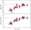 |
Fig. 1 Behaviour of the difference between spectroscopic and |

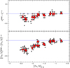 |
Fig. 2 Behaviour of the difference between spectroscopic and |

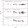 |
Fig. 3 Behaviour of [Fe/H] as a function of χ for individual Fe I lines in three stars in NGC 5904 (upper panel), NGC 1904 (middle panel), and NGC 7099 (lower panel), adopting photometric parameters. Red lines are the linear best fits. The slopes between [Fe/H] and χ are labelled. |
5.2 Sanity checks
We performed some sanity checks to assess the validity of the trends discussed above.
We repeated the analysis using photometric Teff derived from the  – and
– and  –Teff transformations provided by González Hernández & Bonifacio (2009). The average differences between spectroscopic Teff and those obtained from these two additional colours are shown in Fig. 4 as red circles: the behaviour with the metallicity closely resembles that seen for
  . The observed run of the differences of the parameters with the metallicity is independent of the adopted colours.
We checked whether the observed trend is due to the adopted colour–Teff transformations by González Hernández & Bonifacio (2009). We re-analysed the target stars using the Alonso et al. (1999) relations that provide colour–Teff transformations for  ,
,  ,
,  ,
,  and
and  . We adopted the extinction coefficients by McCall (2004), the optical UBVI magnitudes from Stetson et al. (2019), and the near-infrared JKs magnitudes from the 2MASS survey (Skrutskie et al. 2006). The latter were transformed into Telescopio Carlos Sanchez photometric system adopted by Alonso et al. (1999) using the relations by Carpenter (2001). The results are shown in Fig. 4 as blue triangles. The Alonso et al. (1999) scale is cooler than that by González Hernández & Bonifacio (2009) by 47 K (σ = 35 K), 105 K (σ = 11 K) and 83 K (σ = 17 K) for
  ,
,  and
and  , respectively. Despite these differences between the two scales, the same behaviour with the metallicity is found, indicating that this run is not an artefact of the adopted Teff scale.
The target stars were re-analysed by excluding Fe I lines with χ < 2 eV. These lines are more affected by inadequacies in the model atmospheres, in particular 3D effects (Bergemann et al. 2012; Dobrovolskas et al. 2013). A similar selection has been adopted in other studies, albeit with different thresholds (see e.g. Cayrel et al. 2004; Cohen et al. 2008; Yong et al. 2013; Ruchti et al. 2013). Spectroscopic Teff derived ruling out the low-energy transitions continue to be significantly lower (by ~200–300 K) than the photometric ones for stars with [Fe I/H] < –2.0 dex. As clearly visible in the lower panel of Fig. 3, significant values of σχ (~0.07–0.10 dex eV−1) are found in metal-poor stars also when the low-energy Fe I lines are excluded. The inclusion of ten low-χ lines with higher abundances decreases vt by ~0.3 km s−1 (because the excluded transitions are on average the strongest ones and hence the most sensitive to vt) but has a negligible impact on the average [Fe I/H] because of the large number of high-energy lines in our line list.
The determination of spectroscopic log g can be affected by the choice of the used gf values of the Fe II lines because the latter are less precise than those available for Fe I lines and laboratory values are only available for a few lines. We checked two alternative sets of Fe II gf values: the laboratory oscillator strengths provided by Kroll & Kock (1987), Heise & Kock (1990) and Hannaford et al. (1992) and the theoretical ones by Raassen & Uylings (1998).
Gravities obtained assuming the laboratory values are compatible, within the uncertainties, with those obtained adopting the values by Meléndez & Barbuy (2009), with an average difference (laboratory - this work) of –0.03 dex (σ = 0.09 dex). On the other hand, gravities obtained with theoretical gf values are lower than those we obtain, with an average difference of –0.28 dex (σ = 0.13 dex), increasing the discrepancy between the photometric and spectroscopic log g. In both cases, spectroscopic Teff and vt are not affected by the choice of the gf values of Fe II lines. These checks demonstrate that the strong difference between spectroscopic and photometric log g shown in Fig. 1 cannot be attributed to the uncertainties in the adopted gf values of Fe II lines.
Finally we checked whether the adoption of a different combination of model atmospheres and spectral synthesis code can alleviate or solve the observed discrepancies. We repeated the analysis using the code TURBOSPECTRUM (Plez 2012) coupled with the MARCS model atmospheres (Gustafsson et al. 2008) but this choice does not change the observed runs.
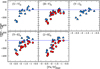 |
Fig. 4 As in Fig. 1 but this time adopting the relations by Alonso et al. (1999, blue triangles) for the colours |


6 Previous works
This work presents for the first time a homogeneous comparison between the two approaches used to derive stellar parameters and performed on the entire metallicity range of the Galactic GCs. The analysis of individual metal-poor clusters is not sufficient to highlight the overall behaviour that we have identified because the difference between photometric and spectroscopic parameters can be interpreted as an effect of systematic errors (and not as a metallicity-dependent phenomenon). However, hints of a similar behaviour were found in some previous works analysing GCs with different metallicities.
Carretta et al. (2009b) analysed 202 giant stars in 17 GCs observed with UVES-FLAMES@VLT, adopting photometric parameters and finding that σχ turn out to be more negative in metal-poor stars. These latter authors provided an average slope σχ =−0.013 dex eV−1 (σ = 0.029 dex eV−1) suggesting that the photometric Teff should be decreased by 45 K to obtain an average, null σχ. This approach interprets the average slope as being the result of an offset between spectroscopic and photometric Teff, while the effect becomes significant only at low metallicity. In particular, Carretta et al. (2009b) found slopes of −0.04/−0.07 dex/eV for the GCs with [Fe/H] < −2.0 dex; these values are higher than those obtained in our work with the González Hernández & Bonifacio (2009) relations but are compatible with those that we found with the Alonso et al. (1999) transformations (the same used by Carretta et al. 2009b).
Nidever et al. (2020) in their study on the chemical composition of giant stars in the Magellanic Clouds compared the iron content of 14 southern Galactic clusters observed with APOGEE-2S with the values listed by Carretta et al. (2009b). We recall that the analysis by Carretta et al. (2009b) is based on photometric parameters while the atmospheric parameters for the APOGEE-2S targets were derived from the ASPCAP pipeline (García Pérez et al. 2016) by fitting the observed spectra with synthetic ones in specific spectral regions sensitive to one or more parameters. The agreement is satisfactory down to [Fe/H] ~ –2.0 dex, while for the most metal-poor clusters the iron abundance for the spectroscopic parameters by ASPCAP is lower by ~0.2 dex than the iron content derived by Carretta et al. (2009b). Because of the different wavelength range and the use of different diagnostics, identification of the origin of this discrepancy between optical and near-infrared GC metallicities is not trivial, in particular because no comparison of Teff and log g for the stars in common is discussed. However, a more accurate comparison between the two analyses should be performed to understand whether the discrepancy highlighted by Nidever et al. (2020) for the metal-poor GCs is due to the different methods used to estimate the atmospheric parameters or other effects related to the different spectral ranges. For a more detailed comparison between near-infrared spectroscopic and photometric Teff we refer the reader to Mészáros et al. (2015, 2020), Jönsson et al. (2018), and Masseron et al. (2019).
Kovalev et al. (2019) analysed some open and globular clusters determining stellar parameters by comparing the observed spectra with both LTE and NLTE synthetic spectra. The differences in Teff and log g between the LTE and NLTE analyses, both based on spectroscopic diagnostics and not photometric parameters, are qualitatively analogous to those obtained in this work; in particular, for clusters with [Fe/H] < –2.0 dex, these latter authors found that LTE spectroscopic Teff and log g are lower than the NLTE ones by ~200–300 K and 0.4–0.6 dex, respectively.
7 Discussion
7.1 Which parameter set should be preferred for metal-poor giant stars?
As explained in Sect. 1, one of the main advantages of working with GCs is that we can easily compare the atmosphericparameters (derived from photometry or spectroscopy) with the values predicted by appropriated theoretical isochrones. This provides a powerful and exemplary check to decide whether a given set of parameters is correct or not, because it should be consistent with the position of the star in the CMD.
Figure 5 shows the position of the individual GC stars in the Teff – log g diagram (red and blue circles are the photometric and spectroscopic parameters, respectively), with the corresponding best-fit theoretical DARTMOUTH isochrone superimposed. The photometric parameters closely match those predicted by the isochrones. On the other hand, the position of the stars when the spectroscopic parameters are adopted shifts systematically toward lower Teff and log g decreasing the cluster metallicity.
A simple argument in favour of photometric parameters is that the spectroscopic ones predict an incorrect position in the Teff – log g diagram for the latter-mentioned stars. For most of the investigated GCs, the target stars are 1–3 magnitudes fainter than the RGB tip, while the spectroscopic parameters locate them close to the tip of the RGB.
As a simple and quantitative test, we compared the luminosities derived from the observed magnitudes with those predicted according to the spectroscopic parameters. The stellar luminosity of each target star has been calculated both from the observed V-band magnitude as described in Sect. 3.1 and adopting the spectroscopic Teff and log g. Figure 6 shows the behaviour of the difference between the two luminosities as a function of the metallicity (the corresponding magnitude difference is also shown in the right vertical axis). Spectroscopic parameters predict luminosities higher than the observed ones and this difference increases toward lower metallicities. In terms of magnitude, the most metal-poor GC stars should be ~2.5 magnitudes brighter than the observed V-band magnitudes. This demonstrates that the spectroscopic parameters for metal-poor giant stars are not consistent with the evolutionary stage of the stars as inferred from their position in the CMD. Hence, the spectroscopic parameters are not reliable, locating the stars in a discrepant position in the Teff – log g diagram.
7.2 Technical origin of the parameter discrepancy
The discrepancy between the spectroscopic and photometric parameters is mainly driven by the discrepancy in Teff, which also causes discrepancies between log g and vt (and hence in [Fe/H]). Figure 7 explains how a spurious, non-null σχ value also leads to an incorrect result in terms of log g and metallicity, locating the stars in an incorrect position of the Teff – log g diagram.
We consider the star NGC 4590-3584 that has photometric parameters Teff = 4831 K and log g = 1.65 (marked as a red large circle in the Teff – log g diagram in the main panel of Fig. 7). The photometric Teff does not satisfy the excitation equilibrium, providing a slope of σχ = −0.09 ± 0.01 dex eV−1, while abundances from neutral and single ionised lines are compatible each other ([Fe I/Fe II] = 0.0 dex).
In order to null σχ, Teff needs to be decreased by ~400 K (green circle in the main panel). However, a change in Teff impacts both Fe I and Fe II lines, albeit in opposite directions. In particular, a decrease in Teff by 100 K decreases the abundance from Fe I lines but increases that by Fe II lines, leading to a decrease of [Fe I/Fe II] by about 0.18 dex and therefore to a decrease of log g by about 0.3 dex. In the case of the star shown in Fig. 7, a decrease in Teff of ~400 K leads to [Fe I/Fe II] = −0.59 dex and we need to decrease log g by 1.2 dex in order to fulfil the ionisation equilibrium (blue circle in the main panel).
We note that the star NGC 4590-3584 is ~1.8 magnitudes fainter than the RGB Tip but it should be located close to the RGB Tip according to its spectroscopic parameters. This confirms that the spectroscopic parameters of this star are incorrect even if they fulfil both ionisation and excitation balance.
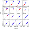 |
Fig. 5 Behaviour of log g as a function of Teff for all the target clusters (sorted by increasing metallicity); blue points are the spectroscopic parameters and red points the photometricones. For each cluster the corresponding best-fit DARTMOUTH theoretical isochrone is shown (grey solid line). |
7.3 Physical origin of the parameter discrepancy
Now that we have demonstrated that the spectroscopic parameters are not reliable for metal-poor giant stars, we feel it necessary to find the physical origin of this discrepancy. The fact that the differences between the two sets of parameters increase at lower metallicities suggests that these effects are due to inadequacies of the standard model atmospheres and/or spectral synthesis codes and in particular the assumptions of 1D geometry and LTE.
We verified that NLTE effects, under the assumption of 1D geometry, are not sufficient to alleviate the parameter discrepancy. We applied the NLTE corrections provided by Bergemann et al. (2012)4 to the Fe I lines of the three stars shown in Fig. 3. We found that for the stars NGC 5904-900073 and NGC 904-171 the slopes of σχ do not significantly change, while for NGC 7099-7414 a non-null σχ remains, indicating that a significant decrease of Teff is requested also with 1D/NLTE abundances. This finding is compatible with the analysis performed by Amarsi et al. (2016) on the metal-poor giant star HD 122563, which shows a similar, negative σχ both in 1D/LTE and 1D/NLTE (see their Fig. 2).
On the other hand, 3D effects mainly impact low χ lines (see e.g. Collet et al. 2007; Dobrovolskas et al. 2013; Amarsi et al. 2016). The star HD 122563 discussed by Amarsi et al. (2016) has parameters and metallicities comparable with the most metal-poor stars studied here. The 3D/LTE analysis is able to invert the observed trend between Fe abundance and χ providing a positive σχ. However, the 3D/NLTE analysis provides again a negative slope (albeit less steeply negative than that obtained in the 1D/LTE case) because the NLTE effects counterbalance the 3D effects. The results provided by Amarsi et al. (2016) seem to suggest that a 3D/NLTE analysis could partially reduce the discrepancy between the spectroscopic and photometric parameters. However, this approach still does not provide a flat behaviour between Fe abundance and χ, suggesting that our current modelling of 3D/NLTE effects in metal-poor giant stars is still incomplete.
Among the current shortcomings of available 3D model atmospheres, we highlight the coarse treatment of opacity (with respect to what is possible in 1D model atmospheres) and the incomplete treatment of scattering. Currently, 3D model atmospheres either treat scattering as true absorption (e.g. all the older CO5BOLD models of the CIFIST grid of Ludwig et al. 2009) or they use an approximate treatment, usually called the Hayek approximation (Hayek et al. 2010), which consists in treating scattering as true absorption in the optically thick layers and ignoring it in the optically thin layers. The effects of the two approximations on the emergent fluxes are discussed in Bonifacio et al. (2018). However no investigation has been done of the impact of the different approximations on line formation. We stress that at present no grid of 3D model atmospheres with a full treatment of scattering is available, such as the one constructed by Hayek et al. (2010). Another possible limitation of the current generation of 3D model atmosphere grids, such as the two most popular examples, the CIFIST grid (Ludwig et al. 2009)and the STAGGER grid (Magic et al. 2013), is that they use the opacity package of the MARCS 1D models (Gustafsson et al. 2008), which was created to compute models with effective temperatures below 8000 K. This implies that there are no opacities for temperatures in excess of 30 000 K. While such very high temperatures are not encountered in any layer of 1D models cooler than 8000 K, in 3D hydro models of cool stars one often finds temperatures that exceed this value, and the codes are obliged to take a bold extrapolation in the opacities.
Although there is a general consensus that NLTE effects are indeed important in the line formation of metal-poor stars, we are also aware that the calculations are more complex and rely on input from atomic physics. Although we believe that the current NLTE computations for Fe are the state of the art, there is still the possibility that shortcomings remain. One such example that we are aware of is that some physical process that may contribute to populating or depopulating atomic levels has either been ignored or included with an incorrect cross-section (e.g. charge transfer). A common uncertainty is provided by the collisions with neutral hydrogen. The very sophisticated calculation of Amarsi et al. (2016) does take advantage of quantum mechanical computations for the Fe + H collision rates and includes charge-transfer reactions that lead to Fe+ + H−. Concerning the collisions of hydrogen with Fe II, Amarsi et al. (2016) adopted the unphysical Drawin recipe (Drawin 1968, 1969), due to the lack of availability of the relevant quantum-mechanical computations. Another issue of concern surrounding the use of NLTE computations (both in 1D or in 3D) is that the wavelength resolution must be high enough to correctly compute the wings of thestrong UV lines that in many atoms effectively control the population. A computation that is too coarse may produce incorrect results. Computations are usually checked against the Sun and Arcturus, however these checksdo not guarantee that there will not be any shortcomings when computing the line formation in a metal-poor giant.
The final concern we mention here refers to the possible effects of NLTE on the structure of a 3D model. Both CO5BOLD and STAGGER assume LTE in the model computation, NLTE is only taken into account when computing line formation using a fixed background model. This is a reasonable assumption, but could be the cause of the above-mentioned shortcomings.
In our view, the fact that the most advanced 3D-NLTE computations of Amarsi et al. (2016) for the metal-poor giant HD 122563 are unable to remove a slope of abundance versus excitation temperature demonstrates that even when using such sophisticated computations, the excitation temperature is unreliable for a metal-poor giant.
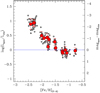 |
Fig. 6 Behaviour of the ratio between the luminosities derived from spectroscopic and photometric parameters as a function of [Fe/H] (the latter derived from photometric parameters). The right vertical axis shows the difference in terms of magnitude. The same symbols are used as in Fig. 1. |
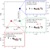 |
Fig. 7 Scheme of the location of the star NGC 4590-3584 in the Teff– log g plane (main panel) according to different chemical analyses: the red circle indicates the photometric parameters, the green circle the position of the star when the constraint of null σχ is fulfilled, and the blue circle the position of the star according to the spectroscopic determination of the parameters. For each of these (Teff, log g) pairs, the run of [Fe/H] as a function of χ is shown (both neutral and single ionised lines shown as black and red circles, respectively). |
8 A correction scheme for atmospheric parameters
In view of the above discussion, we want to provide ready-to-use empirical recipes that will result in accurate atmospheric parameters for giant stars, placing them in the correct place in a Hertzsprung–Russel diagram.
8.1 RGB stars with [Fe/H] > −1.5 dex
For RGB stars with [Fe/H] ≿ −1.5 dex, the spectroscopic and photometric approaches are equivalent and the choice of the method is driven by the quality of the available photometry and spectra. However, the spectroscopic method should be avoided when (1) the spectral coverage does not provide a large number of Fe I lines well distributed in χ and/or line strength, introducing errors in Teff and vt ; or (2) only a small number of Fe II lines are available, preventing precise determination of log g. For these stars, the lines with χ < 2 eV can be used because they provide abundances that are coherent with those from high-energy lines, regardless of the approach used to derive Teff.
Microturbulent velocities must to be derived from the spectra and this parameter is heavily affected by the EW distribution of the available Fe I lines. As already done by other works (see e.g. Monaco et al. 2005; Kirby et al. 2009), we provide a linear relation between vt and log g in order to determine this parameter, even in the case of spectra inadequate for this task. As visible in Fig. 8, where the run of vt as a function of log g for all the individual stars is shown, there are two evident sequences depending on the metallicity. For the stars with [Fe/H] > −2.1 dex, vt can be calculated with the following relation:
 (1)
(1)
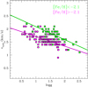 |
Fig. 8 Behaviour of vt as a function of log g for the individual stars: purple and green squares are the stars in the GCs with [Fe/H] >−2.1 dex and [Fe/H] < −2.1 dex, respectively. Purple and green thick lines are the best linear fits on the two samples of stars. |
8.2 RGB stars with [Fe/H] < −1.5 dex
For RGB stars with [Fe/H] ≾ −1.5 dex, the photometric approach should always be adopted, even if the available spectra allow precise determination of the parameters. Sometimes the spectroscopic parameters can be more precise (even if less accurate) than the photometric ones because of the low quality of the available photometry, the uncertainty in the colour excess, or the presence of differential reddening. For these cases, the spectroscopic parameters can be the only feasible route. In order to bypass the issues in the spectroscopic parameters discussed above, we provide a linear relation between the iron abundance obtained with the spectroscopic parameters [Fe/H]spec and the average ΔTeff from the broad-band colours, both using the relations by González Hernández & Bonifacio (2009) and Alonso et al. (1999), as shown in the upper and lower panel in Fig. 9, respectively.
![Mathematical equation: \begin{align*} {T_{\textrm{eff}}^{GB09}} \!= T_{\textrm{eff}}^{\textrm{spec}} - (264\pm33)\cdot{\textrm{[Fe/H]}_{\textrm{spec}}}-(358\pm70) (\sigma=36\, \textrm{K}), \end{align*}](/articles/aa/full_html/2020/08/aa37703-20/aa37703-20-eq22.png) (2)
(2)
![Mathematical equation: \begin{align*} {T_{\textrm{eff}}^{A99}} = T_{\textrm{eff}}^{\textrm{spec}} - (240\pm28)\cdot{\textrm{[Fe/H]}_{\textrm{spec}}}-(385\pm60) (\sigma=31 \,\textrm{K}). \end{align*}](/articles/aa/full_html/2020/08/aa37703-20/aa37703-20-eq23.png) (3)
(3)
We note that the relations by Alonso et al. (1999) provide an excellent match with the spectroscopic Teff for stars with [Fe/H] > –1.5 dex, while an offset of ~50 K remains when we use those of González Hernández & Bonifacio (2009). On the other hand, Alonso et al. (1999) provide lower Teff for the metal-poor clusters with respect to theoretical isochrones, while González Hernández & Bonifacio (2009) provide a good match with the isochrones at all metallicities.
Because these relations are defined only for RGB stars in the metallicity range –2.5 < [Fe/H] < –1.5 dex, we checked whether or not they also work at lower metallicities. We analysed four RGB field stars with metallicities between approximately −3.5 and −2.5 dex, namely HE 0305-452, CD 38245, HD 122563, and HE 2141-3741. For these stars we retrieved archival spectra acquired with the spectrograph UVES@VLT, adopting the photometry available in the SIMBAD database (Wenger et al. 2000), colour excess from Schlafly & Finkbeiner (2011) and parallaxes from Gaia Data Release 2 (Gaia Collaboration 2016, 2018). Photometric and spectroscopic parameters and corresponding [Fe I/H] are listed in Table 4. Also for these stars, significant slopes σχ are found when the photometric Teff are adopted, leading to lower spectroscopic Teff. Additionally, the spectroscopic log g are significantly lower than the photometric ones, that is, by about 1 dex. The precision of the Gaia parallaxes is of about 20% for HE 0305-452, CD 38245, and HE 2141-3741, and 3% for HD 122563. However, the precision of the parallax in the first three stars changes the photometric gravities by about 0.2 dex. The use of the Gaia parallaxes is unable to reconcile photometric and spectroscopic log g. The spectroscopic Teff corrected with the relations defined from GCs closely match the photometric Teff, demonstrating that these relations can be extrapolated at lower metallicities and used for very metal-poor RGB field stars (at least down to [Fe/H] ~−3.5 dex), especially when no precise photometry and/or colour excess are available.
Concerning the determination of gravities, for [Fe/H] < −1.5 dex, spectroscopic log g should be avoided because the [Fe I/Fe II] ratio is more sensitive to Teff than to log g. Hence, if the spectroscopic Teff is incorrect, the spectroscopic log g also turns out to be incorrect due to the opposite sensitivity of Teff for Fe I and Fe II (see Fig. 7). A more robust and safe approach is to use the Teff – log g relation provided by a theoretical isochrone (when the age is well known, as in the case of a GC) or to recalculate gravities adopting the corrected Teff. In this case we offer the following warning: to derive log g, a rough estimate of the mass of the star is needed. If we exclude the cases for which the mass is otherwise known (binary stars, stars with asteroseismic data...), the mass estimate hinges on the age estimate. If we know the star is old (say older than 10 Gyr), as in the case of GCs, we can safely assume a mass of ~0.7–0.8 M⊙. If however the star is younger than 1 Gyr, its mass can be as large as 5 M⊙ leading to a difference of 0.7 dex in the estimated gravity for the same effective temperature (see Lombardo et al., in prep.).
Concerning the determination of vt, the stars down to [Fe/H] ~−2.1 dex follow the same linear relation provided above, while for the stars in the three most metal-poor GCs (NGC 7078, NGC 4590 and NGC 7099, [Fe/H] < –2.1 dex) we provide the following relation:
 (4)
(4)
This different behaviour for the most metal-poor stars is due to the largest Teff discrepancy observed among these stars (see Fig. 1): because the low-χ lines are the strongest ones, vt is increased to partially compensate for the negative slope between abundances and χ.
Finally, we note that for these stars the lines with low energy (<2 eV) should be used with caution. As discussed above, the inclusion of ten low-χ Fe I lines does not significantly impact the average [Fe I/H] (at least for the optical spectra investigated here where the bulk of the Fe I lines includes high-χ lines). However, this cut can impact the abundance of other species for which mainly low-χ are available. For instance, in the optical range covered by the UVES-FLAMES spectra discussed in this work, almost all the Ti lines have χ < 2 eV and the adoption of a threshold in χ can dramatically impact its abundance.
Finally, we recall that Ti provides a significant number of neutral and singly ionised lines, providing an additional diagnostic for the gravities. When the spectroscopic parameters are used, and [Fe I/H] and [Fe II/H] are consistent within the uncertainties by construction, [Ti I/H] is lower than [Ti II/H] by about 0.2 dex. This implies that the gravities should be further decreased in order to match [Ti I/H] and [Ti II/H], worsening the discrepancy with the photometric values. We suspect that this behaviour is due to the low χ of all the available Ti lines. The latter are extremely sensitive to the inadequacies of the model atmospheres, in particular to NLTE effects, as demonstrated by Mashonkina et al. (2016), finding that, at [M/H] = −2.0 dex, the NLTE corrections for the Ti I lines are larger than those for the Fe I lines.
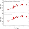 |
Fig. 9 Behaviour of the average difference between the spectroscopic and photometric Teff obtained from individual colours for target clusters (red circles) as a function of the iron abundance derived adopting spectroscopic parameters. The values of Teff in the upper and lower panels were obtained with the relations of González Hernández & Bonifacio (2009) and Alonso et al. (1999), respectively. The vertical errorbars are the dispersions of the mean for Teff for each cluster. Thick grey lines are the best linear fits obtained for the clusters with [Fe/H] < –1.5 dex. |
Field metal-poor giant stars with the atmospheric parameters and [Fe I/H] derived adopting photometric and spectroscopicparameters.
9 Summary and conclusions
The analysis of a sample of 16 Galactic GCs observed with UVES-FLAMES@VLT using two different approaches to derive the parameters leads to the following results:
-
The discrepancy between spectroscopic and photometric parameters for giant stars increases with decreasing metallicity. This behaviour is confirmed when adopting different broad-band colours or colour–Teff transformations. Such a difference between the two sets of parameters cannot be interpreted as simply being due to systematic error.
-
The spectroscopic approach based on excitation and ionisation balances provides incorrect stellar parameters for metal-poor stars, in particular leading to overly low Teff and log g, inconsistent with the values predicted by appropriate theoretical isochrones and with the observed position of the stars in the CMD.
-
The discrepancy between the two approaches seems to arise from inadequacies of the adopted physics. In particular, low-energy lines are the most prone to 3D effects (Bergemann et al. 2012; Dobrovolskas et al. 2013; Amarsi et al. 2016) and the use of 1D model atmospheres is likely responsible for the negative values of σχ that lead to overly low Teff and log g. On the other hand, neither 1D/NLTE nor 3D/NLTE are sufficient to flatten the observed σχ and alleviate the discrepancy between the two parameter sets, at least in the computations currently available.
-
We propose simple relations to correct spectroscopic Teff and put them onto the “photometric” scales described by Alonso et al. (1999) and González Hernández & Bonifacio (2009). These relations are suitable for RGB stars with [Fe/H] < –1.5 dex and they can be used to correct spectroscopic Teff both in GCs and in field stars when no accurate or precise photometry is available.
-
One-dimensional (LTE or NLTE) chemical analyses of RGB stars with [Fe/H] < –1.5 dex and based on spectroscopic parameters should be considered with great caution because the parameters could be underestimated, as could the derived [Fe/H]. We recommend avoiding spectroscopic Teff for these stars and advocate the use of photometric or corrected Teff.
Finally, we stress that both spectroscopic and photometric Teff fail to accurately reproduce the spectral properties of giant stars. Spectroscopic Teff provide, by construction, the same abundance from lines of different χ but clearly fail to reproduce the emerging flux of the stars. On the other hand, IRFM photometric Teff accurately reproduce the bolometric flux but they systematically provide erroneous abundances for the low-energy lines. For 1D chemical analyses, it is necessary to decide which aspect must take precedence, that is, a temperature able to reproduce the emerging stellar flux or one that gives the depths of individual metallic lines.
Our argumentation concerning the position of the stars in the Teff – log g diagram discussed in Sect. 5 is in favour of rejecting the spectroscopic Teff, while we find that the photometric Teff, despite its failure to reproduce the excitation balance, appears to be the best choice.
Nevertheless, the development of more accurate and complete 3D/NLTE tools remains the most likely way to obtain an exhaustive description of the stellar spectra and bypass the issues discussed in this work.
Acknowledgements
We are grateful to the anonymous referee for the useful comments and suggestions. A.M. is grateful to the Scientific Council of Observatoire de Paris that funded his extended visit at GEPI, where part of this work was carried out. This research has made use of the SIMBAD database, operated at CDS, Strasbourg, France and of data from the European Space Agency (ESA) mission Gaia (https://www.cosmos.esa.int/gaia), processed by the Gaia Data Processing and Analysis Consortium (DPAC, https://www.cosmos.esa.int/web/gaia/dpac/consortium). Funding for the DPAC has been provided by national institutions, in particular the institutions participating in the Gaia Multilateral Agreement.
References
- Alonso, A., Arribas, S., & Martinez-Roger, C., 1999, A&A, 140, 261 [Google Scholar]
- Amarsi, A. M., Lind, K., Asplund, M., et al. 2016, MNRAS, 463, 1518 [NASA ADS] [CrossRef] [Google Scholar]
- Baines, E. K., McAlister, H. A., ten Brummelaar, T. A., et al. 2008, ApJ, 682, 577 [NASA ADS] [CrossRef] [Google Scholar]
- Bergemann, M., Lind, K., Collet, R., et al. 2012, MNRAS, 427, 27 [NASA ADS] [CrossRef] [Google Scholar]
- Blackwell, D. E., & Shallis, M. J. 1977, MNRAS, 180, 177 [NASA ADS] [CrossRef] [Google Scholar]
- Blackwell, D. E., Shallis, M. J., & Selby, M. J. 1979, MNRAS, 188, 847 [NASA ADS] [CrossRef] [Google Scholar]
- Blackwell, D. E., Petford, A. D., & Shallis, M. J. 1980, A&A, 82, 249 [NASA ADS] [Google Scholar]
- Bonifacio, P., Caffau, E., Ludwig, H.-G., et al. 2018, A&A, 611, A68 [NASA ADS] [CrossRef] [EDP Sciences] [Google Scholar]
- Boyajian, T. S., McAlister, H. A., Baines, E. K., et al. 2008, ApJ, 683, 424 [NASA ADS] [CrossRef] [Google Scholar]
- Carpenter, J. M. 2001, AJ, 121, 2851 [NASA ADS] [CrossRef] [Google Scholar]
- Carretta, E., Bragaglia, A., Gratton, R., et al. 2009a, A&A, 508, 695 [NASA ADS] [CrossRef] [EDP Sciences] [Google Scholar]
- Carretta, E., Bragaglia, A., Gratton, R., & Lucatello, S. 2009b, A&A, 505, 139 [NASA ADS] [CrossRef] [EDP Sciences] [Google Scholar]
- Casagrande, L., Ramírez, I., Meléndez, J., Bessell, M., & Asplund, M. 2010, A&A, 512, A54 [NASA ADS] [CrossRef] [EDP Sciences] [Google Scholar]
- Castelli, F., & Kurucz, R. L. 2003, IAU Symp., 210, A20 [Google Scholar]
- Cayrel, R., Depagne, E., Spite, M., et al. 2004, A&A, 416, 1117 [NASA ADS] [CrossRef] [EDP Sciences] [Google Scholar]
- Cohen, J. G., Christlieb, N., McWilliam, A., et al. 2008, ApJ, 672, 320. [NASA ADS] [CrossRef] [Google Scholar]
- Collet, R., Asplund, M., & Trampedach, R. 2007, A&A, 469, 687 [NASA ADS] [CrossRef] [EDP Sciences] [Google Scholar]
- Dobrovolskas, V., Kučinskas, A., Steffen, M., et al. 2013, A&A, 559, A102 [NASA ADS] [CrossRef] [EDP Sciences] [Google Scholar]
- Dotter, A., Chaboyer, B., Jevremović, D., et al. 2008, ApJS, 178, 89 [NASA ADS] [CrossRef] [Google Scholar]
- Drawin, H.-W. 1968, Z. Phys., 211, 404 [NASA ADS] [CrossRef] [EDP Sciences] [Google Scholar]
- Drawin, H. W. 1969, Z. Phys., 225, 483 [NASA ADS] [CrossRef] [EDP Sciences] [Google Scholar]
- Frebel, A., Casey, A. R., Jacobson, H. R., et al. 2013, ApJ, 769, 57 [NASA ADS] [CrossRef] [Google Scholar]
- Fuhr, J. R., & Wiese, W. L. 2006, J. Phys. Chem. Ref. Data, 35, 1669 [NASA ADS] [CrossRef] [Google Scholar]
- Kervella, P., & Fouqué, P. 2008, A&A, 491, 855 [NASA ADS] [CrossRef] [EDP Sciences] [Google Scholar]
- Kervella, P., Thévenin, F., Di Folco, E., et al. 2004, A&A, 426, 297 [NASA ADS] [CrossRef] [EDP Sciences] [Google Scholar]
- Kervella, P., Bigot, L., Gallenne, A., et al. 2017, A&A, 597, A137 [NASA ADS] [CrossRef] [EDP Sciences] [Google Scholar]
- Koch, A., & McWilliam, A. 2014, A&A, 565, A23 [NASA ADS] [CrossRef] [EDP Sciences] [Google Scholar]
- Kovalev, M., Bergemann, M., Ting, Y.-S., et al. 2019, A&A, 628, A54 [CrossRef] [EDP Sciences] [Google Scholar]
- Kurucz, R. L. 2005, Mem. Soc. Astron. It. Suppl., 8, 14 [Google Scholar]
- Gaia Collaboration (Prusti, T., et al.) 2016, A&A, 595, A1 [NASA ADS] [CrossRef] [EDP Sciences] [Google Scholar]
- Gaia Collaboration (Brown, A. G. A., et al.) 2018, A&A, 616, A1 [NASA ADS] [CrossRef] [EDP Sciences] [Google Scholar]
- García Pérez, A. E., Allende Prieto, C., Holtzman, J. A., et al. 2016, AJ, 151, 144 [Google Scholar]
- González Hernández, J. I., & Bonifacio, P. 2009, A&A, 497, 497 [NASA ADS] [CrossRef] [EDP Sciences] [Google Scholar]
- Gruyters, P., Lind, K., Richard, O., et al. 2016, A&A, 589, A61 [NASA ADS] [CrossRef] [EDP Sciences] [Google Scholar]
- Gustafsson, B., Edvardsson, B., Eriksson, K., et al. 2008, A&A, 486, 951 [NASA ADS] [CrossRef] [EDP Sciences] [Google Scholar]
- Hannaford, P., Lowe, R. M., Grevesse, N., et al. 1992, A&A, 259, 301 [Google Scholar]
- Harris, W. E. 1996, AJ, 112, 1487 [NASA ADS] [CrossRef] [Google Scholar]
- Hayek, W., Asplund, M., Carlsson, M., et al. 2010, A&A, 517, A49 [NASA ADS] [CrossRef] [EDP Sciences] [Google Scholar]
- Heise, C., & Kock, M. 1990, A&A, 230, 244 [NASA ADS] [Google Scholar]
- Johnson, J. A. 2002, ApJS, 139, 219 [NASA ADS] [CrossRef] [Google Scholar]
- Jönsson, H., Allende Prieto, C., Holtzman, J. A., et al. 2018, AJ, 156, 126 [NASA ADS] [CrossRef] [Google Scholar]
- Kirby, E. N., Guhathakurta, P., Bolte, M., et al. 2009, ApJ, 705, 328 [NASA ADS] [CrossRef] [Google Scholar]
- Kroll, S., & Kock, M. 1987, A&AS, 67, 225 [NASA ADS] [Google Scholar]
- Lambert, D. L., Heath, J. E., Lemke, M., et al. 1996, ApJS, 103, 183 [NASA ADS] [CrossRef] [Google Scholar]
- Landolt, A. U. 1992, AJ, 104, 340 [NASA ADS] [CrossRef] [Google Scholar]
- Lind, K., Bergemann, M., & Asplund, M. 2012, MNRAS, 427, 50 [NASA ADS] [CrossRef] [Google Scholar]
- Lovisi, L., Mucciarelli, A., Lanzoni, B., et al. 2013, ApJ, 772, 148 [NASA ADS] [CrossRef] [Google Scholar]
- Ludwig, H.-G., Caffau, E., Steffen, M., et al. 2009, Mem. Soc. Astron. It., 80, 711 [Google Scholar]
- Magic, Z., Collet, R., Asplund, M., et al. 2013, A&A, 557, A26 [NASA ADS] [CrossRef] [EDP Sciences] [Google Scholar]
- Martin, G. A., Fuhr, J. R., & Wiese, W. L. 1988, Atomic transition probabilities. Scandium through Manganese (New York: American Institute of Physics (AIP) and American Chemical Society) [Google Scholar]
- Mashonkina, L. I., Sitnova, T. N., & Pakhomov, Y. V. 2016, Astron. Lett., 42, 606 [NASA ADS] [CrossRef] [Google Scholar]
- Masseron, T., García-Hernández, D. A., Mészáros, S., et al. 2019, A&A, 622, A191 [NASA ADS] [CrossRef] [EDP Sciences] [Google Scholar]
- McCall, M. L. 2004, AJ, 128, 2144 [NASA ADS] [CrossRef] [Google Scholar]
- Meléndez, J., & Barbuy, B. 2009, A&A, 497, 611 [NASA ADS] [CrossRef] [EDP Sciences] [Google Scholar]
- Monaco, L., Bellazzini, M., Bonifacio, P., et al. 2005, A&A, 441, 141 [NASA ADS] [CrossRef] [EDP Sciences] [MathSciNet] [Google Scholar]
- Mészáros, S., Martell, S. L., Shetrone, M., et al. 2015, AJ, 149, 153 [NASA ADS] [CrossRef] [Google Scholar]
- Mészáros, S., Masseron, T., García-Hernández, D. A., et al. 2020, MNRAS, 492, 1641 [CrossRef] [Google Scholar]
- Mucciarelli, A., 2013, ArXiv e-prints [arXiv:1311.1403] [Google Scholar]
- Mucciarelli, A., Pancino, E., Lovisi, L., Ferraro, F. R., & Lapenna, E., 2013a, ApJ, 766, 78 [NASA ADS] [CrossRef] [Google Scholar]
- Mucciarelli, A., Bellazzini, M., Catelan, M., et al. 2013b, MNRAS, 435, 3667 [NASA ADS] [CrossRef] [Google Scholar]
- Mucciarelli, A., Lapenna, E., Massari, D., Ferraro, F. R., & Lanzoni, B. 2015, ApJ, 801, 69 [NASA ADS] [CrossRef] [Google Scholar]
- Mucciarelli, A., Lapenna, E., Lardo, C., et al. 2019, ApJ, 870, 124 [CrossRef] [Google Scholar]
- Nidever, D. L., Hasselquist, S., Hayes, C. R., et al. 2020, ApJ, 895, 88 [CrossRef] [Google Scholar]
- Plez, B. 2012, Astrophysics Source Code Library [record ascl:1205.004] [Google Scholar]
- Raassen, A. J. J., & Uylings, P. H. M. 1998, A&A, 340, 300 [Google Scholar]
- Ramírez, I., & Meléndez, J. 2005, ApJ, 626, 446 [NASA ADS] [CrossRef] [MathSciNet] [Google Scholar]
- Ruchti, G. R., Bergemann, M., Serenelli, A., et al. 2013, MNRAS, 429, 126 [NASA ADS] [CrossRef] [Google Scholar]
- Sbordone, L., Bonifacio, P., Castelli, F., & Kurucz, R. L. 2004, Mem. Soc. Astron. It., 5, 93 [Google Scholar]
- Schlafly, E. F., & Finkbeiner, D. P. 2011, ApJ, 737, 103 [NASA ADS] [CrossRef] [Google Scholar]
- Skrutskie, M. F., Cutri, R. M., Stiening, R., et al. 2006, AJ, 131, 1163 [NASA ADS] [CrossRef] [Google Scholar]
- Stetson, P. B., & Pancino, E., PASP, 120, 1332 [Google Scholar]
- Stetson, P. B., Pancino, E., Zocchi, A., Sanna, N., & Monelli, M. 2019, MNRAS, 485, 3042 [NASA ADS] [CrossRef] [Google Scholar]
- Wenger, M., Ochsenbein, F., Egret, D., et al. 2000, A&AS, 143, 9 [NASA ADS] [CrossRef] [EDP Sciences] [Google Scholar]
- Yong, D., Norris, J. E., Bessell, M. S., et al. 2013, ApJ, 762, 26 [NASA ADS] [CrossRef] [Google Scholar]
A(Fe) =  +12.
+12.
All Tables
Spectroscopic dataset of the target globular clusters (sorted in increasing metallicity), including the number of analysed stars, the colour excess, the V-band distance modulus, and the corresponding ESO program.
Average iron abundances for the target clusters derived from photometric parameters (from Fe I and Fe II lines) and from spectroscopic parameters (from Fe I lines).
Average differences between spectroscopic and photometric parameters for each target cluster.
Field metal-poor giant stars with the atmospheric parameters and [Fe I/H] derived adopting photometric and spectroscopicparameters.
All Figures
|
Fig. 1 Behaviour of the difference between spectroscopic and |
| In the text | |
|
Fig. 2 Behaviour of the difference between spectroscopic and |
| In the text | |
|
Fig. 3 Behaviour of [Fe/H] as a function of χ for individual Fe I lines in three stars in NGC 5904 (upper panel), NGC 1904 (middle panel), and NGC 7099 (lower panel), adopting photometric parameters. Red lines are the linear best fits. The slopes between [Fe/H] and χ are labelled. |
| In the text | |
|
Fig. 4 As in Fig. 1 but this time adopting the relations by Alonso et al. (1999, blue triangles) for the colours |
| In the text | |
|
Fig. 5 Behaviour of log g as a function of Teff for all the target clusters (sorted by increasing metallicity); blue points are the spectroscopic parameters and red points the photometricones. For each cluster the corresponding best-fit DARTMOUTH theoretical isochrone is shown (grey solid line). |
| In the text | |
|
Fig. 6 Behaviour of the ratio between the luminosities derived from spectroscopic and photometric parameters as a function of [Fe/H] (the latter derived from photometric parameters). The right vertical axis shows the difference in terms of magnitude. The same symbols are used as in Fig. 1. |
| In the text | |
|
Fig. 7 Scheme of the location of the star NGC 4590-3584 in the Teff– log g plane (main panel) according to different chemical analyses: the red circle indicates the photometric parameters, the green circle the position of the star when the constraint of null σχ is fulfilled, and the blue circle the position of the star according to the spectroscopic determination of the parameters. For each of these (Teff, log g) pairs, the run of [Fe/H] as a function of χ is shown (both neutral and single ionised lines shown as black and red circles, respectively). |
| In the text | |
|
Fig. 8 Behaviour of vt as a function of log g for the individual stars: purple and green squares are the stars in the GCs with [Fe/H] >−2.1 dex and [Fe/H] < −2.1 dex, respectively. Purple and green thick lines are the best linear fits on the two samples of stars. |
| In the text | |
|
Fig. 9 Behaviour of the average difference between the spectroscopic and photometric Teff obtained from individual colours for target clusters (red circles) as a function of the iron abundance derived adopting spectroscopic parameters. The values of Teff in the upper and lower panels were obtained with the relations of González Hernández & Bonifacio (2009) and Alonso et al. (1999), respectively. The vertical errorbars are the dispersions of the mean for Teff for each cluster. Thick grey lines are the best linear fits obtained for the clusters with [Fe/H] < –1.5 dex. |
| In the text | |
Current usage metrics show cumulative count of Article Views (full-text article views including HTML views, PDF and ePub downloads, according to the available data) and Abstracts Views on Vision4Press platform.
Data correspond to usage on the plateform after 2015. The current usage metrics is available 48-96 hours after online publication and is updated daily on week days.
Initial download of the metrics may take a while.