| Issue |
A&A
Volume 640, August 2020
|
|
|---|---|---|
| Article Number | A60 | |
| Number of page(s) | 7 | |
| Section | Interstellar and circumstellar matter | |
| DOI | https://doi.org/10.1051/0004-6361/202037518 | |
| Published online | 11 August 2020 | |
The diffuse gamma-ray emission toward the Galactic mini starburst W43
1
Department of Astronomy, School of Physical Sciences, University of Science and Technology of China,
Hefei,
Anhui
230026,
PR China
e-mail: yangrz@ustc.edu.cn
2
CAS Key Labrotory for Research in Galaxies and Cosmology, University of Science and Technology of China,
Hefei,
Anhui
230026,
PR China
3
School of Astronomy and Space Science, University of Science and Technology of China,
Hefei,
Anhui
230026,
PR China
4
Max-Planck-Institut für Astronomie,
Königstuhl 17,
69117
Heidelberg,
Germany
Received:
16
January
2020
Accepted:
16
June
2020
In this paper we report the Fermi Large Area Telescope (Fermi-LAT) detection of the γ-ray emission toward the young star forming region W43. Using the latest source catalog and diffuse background models, the extended γ-ray excess is detected with a significance of ~16σ. The γ-ray emission has a spectrum with a photon index of 2.3 ± 0.1. We also performed a detailed analysis of the gas content in this region by taking into account the opacity correction to the HI gas column density. The total cosmic-ray (CR) proton energy is estimated to be on the order of 1048 erg, assuming the γ-rays are produced from the interaction of the accelerated protons and nuclei with the ambient gas. Comparing this region to the other star formation regions in our Galaxy, we find that the CR luminosity is better correlated with the wind power than the star formation rate (SFR). This result suggests that CRs are primarily accelerated by stellar wind in these systems.
Key words: gamma rays: ISM / cosmic rays / open clusters and associations: general
© ESO 2020
1 Introduction
The star formation processes are strongly related to cosmic rays (CRs). On the one hand, the CRs are believed to be accelerated by shocks in supernova remnants (SNRs; see, e.g., Blasi 2013) or massive star wind (Aharonian et al. 2019), thus star formation is the ultimate energy source of CRs. On the other hand, CRs control the ionization rate in the core of dense molecular clouds and play an important role in determining the Jeans mass and initial mass function (IMF) of stars (Papadopoulos 2010). On the galactic scale, the derived CR densities are strongly correlated with the star formation rate (SFR) (Ackermann et al. 2012). In this regard, W43 is an ideal location to study the relation between star formation and CRs. W43 is known as a Galactic mini-starburst region (Motte et al. 2003) and contributes about 5–10% of the SFR in the entire Milky Way (Nguyen Luong et al. 2011). The center of W43 is the large H II region W43-main, which is excited by a Wolf-Rayet and OB star cluster. Some γ-ray emissions have also been detected in this region and an extended TeV source has been detected by the HESS telescope H.E.S.S. Collaboration (2018). Acero et al. (2013) have also found GeV excess in this region and attribute it to a potential pulsar wind nebula (PWN), but the powering pulsar has not yet been found. With the improved understanding of the Fermi Large Area Telescope (Fermi-LAT) instrument response and the accumulation of data, it is interesting to revisit the Fermi-LAT observations in this region. Furthermore, Bihr et al. (2015) performed a state-of-the-art analysis of the gas content of this region, and find the optical depth correction is significant for the HI gas column density. Thus it is possible to derive the CR distribution with an unprecedented accuracy.
In this paper, we perform a detailed analysis on the ten-year Fermi-LAT data on this region and investigate the gas and CR content therein. The paper is organized as follows. In Sect. 2 we present the details of the data analysis. In Sect. 3 we investigate the gas distribution in this region. In Sect. 4 we discuss the possible radiation mechanisms of the γ-ray emission in this region. In Sect. 5 we discuss the implications of our observations.
2 Fermi-LAT data analysis
We selected the Fermi-LAT Pass 8 database on the W43 region from August 4, 2008 (MET 239557417), to April 3, 2019 (MET 575964102), for the analysis. To take advantage of a better angular resolution, we discarded PSF 0 event types in the analysis. We chose an A 10° × 10° square region centered at the position of W43 (RA = 281.885°, Dec = −1.942°) as the region of interest (ROI). We used the “source” event class and the recommended data cut expression (DATA_QUAL > 0)&&(LAT_CONFIG == 1) to exclude time periods when spacecraft events affected the data quality. To reduce the background contamination from the Earth’s albedo, only the events with zenith angles less than 90° are included in the analysis. We used the Fermitools from Conda distribution1 together with the latest version of the instrument response functions (IRFs) P8R3_SOURCE_V2 in the analysis.
In our background model, we included the sources in the Fermi-LAT eight-year catalog (4FGL, The Fermi-LAT Collaboration 2020) within the ROI, enlarged by 7°. We left the normalizations and spectral indices free for all sources within 8° of W43. For the diffuse background components, we used the latest Galactic diffuse model gll_iem_v07.fits and isotropic emission model iso_P8R3_SOURCE_V2_v1.txt2 with their normalization parameters free.
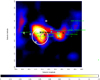 |
Fig. 1 The residual counts map above 10 GeV in the 5° × 5° region near W43, with pixel size of 0.1° × 0.1°, smoothed with a Gaussian filter of 0.2°. The color bars represent the counts per pixel. The white circle is the best-fit uniform disk template. The small black circle marks the position of the star forming region W43-main. The cyan diamonds are the weak sources S1 and S2. The green crosses indicate the point sources listed in the 4FGL. The magenta circle marks the position and size of the TeV source HESS J1848-018. The two black crosses mark the position of the two HESS point sources, HESS J1846-029 (left) and HESS J1844-030 (right), respectively. The white boxes are the positions of the nearby SNRs. |
Fitting results for different models.
2.1 Spatial analysis
Firstly, we used the events above 10 GeV to study the spatial distribution of the γ-ray emissions. We note that there are four unassociated point sources (4FGL J1847.2-0141, 4FGL 1847.2-0200, 4FGL J1849.4-0117, and 4FGL 1850.2-0201) and two identified sources (4FGL 1848.7-0129 identified as GLIMPSE01 and 4FGL 1848.6-0202 identified as NVSS 184840-020408). To study the excess γ-ray emission around W43, we excluded these four unassociated 4FGL sources from our background model. After the likelihood fitting we subtracted the best-fit diffuse model and all the identified sources in the ROI; the resulting residual maps are shown in Fig. 1. We find strong residuals toward the direction of W43-main (marked with a black circle).
To study the morphology of the diffuse emission, we added a disk on top of the model used in the likelihood analysis. We then varied the position and size of the disk to find the best-fit parameters. We compared the overall maximum likelihood of the model with L (alternative hypothesis) and withoutL0 (null hypothesis) uniform disks, and defined the test-statistics (TS) of the disk model − 2(lnL0 −lnL) following Lande et al. (2012). The best-fit result is a disk centered at (RA = 282. °22 ± 0.1, Dec = − 1. ° 65 ± 0.1) with σ = 0.6° ± 0.1 and a TS value of 270, corresponding to a significance of more than 16 σ. We also tested whether or not this extended emission is composed of several independent point sources. To do this we recovered the four unassociated point sources in the likelihood model. The -log(likelihood) function value is larger here than in the 2D disk template case, even with more free parameters. To compare the goodness of the fit in the different models, we also calculated the Akaike information criterion (AIC) values for each model. The AIC was defined as AIC = −2log(likelihood) + 2k, where k is the number of free parameters in the model. We list the -log(likelihood) and corresponding AIC values in Table 1. We also note that the morphology of the residual hints at a deviation from a simple disk; we tried to fit the residual with Gaussian and elliptical templates but found no significant improvement. Thus in the following analysis we used the best-fit disk as the spatial template.
The derived photon index above 10 GeV is 2.27 ± 0.14 and the total γ-ray flux can be estimated as (6.1 ± 0.7) × 10−10 ph cm−2 s−1 above 10 GeV, which reads (2.8 ± 0.4) × 1035 erg s−1 above 1 GeV, if we assume a distance of 5.5 kpc (Zhang et al. 2014) and a single power law spectrum. We find two other residuals to the west (right) of W43, which are marked as S1 and S2 in the residual map. Although adding point sources to the corresponding region does not significantly improve the likelihood (the TS for S1 and S2 are 12 and 10, respectively), we included these two point sources in the following analysis. There are three HESS TeV γ-ray sources in this region, which are HESS J1848-018, HESS J1846-029, and HESS J1844-030. The positions of the HESS sources are also marked in Fig. 1.
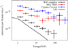 |
Fig. 2 The SED of γ-ray emission toward W43 for a uniform disk spatial model with a radius of 0.6°, normalized to emissivity per H atom. The distance of 5.5 kpc is used and the masses are derived in Sect. 3. The solid curve represents the spectrum of emissivity per H atom, assuming the energy distribution of protons is the same as the local intestellar spectrum (LIS) (Casandjian 2015). Also plotted are the normalized SEDs of the Cygnus cocoon (Aharonian et al. 2019) and NGC 3603 (Yang & Aharonian 2017). |
2.2 Spectral analyses
To further investigate the spectral property of the GeV emission toward W43 and the underlying particle spectra, we fixed the 0.6° uniform circle disk as the spatial model of the extended γ-ray emission and used a power law function to model the spectral shape.
We divided the energy range 1–300 GeV into nine logarithmically spaced energy bins and derived the spectral energy distribution (SED) via the maximum likelihood analysis in each energy bin. The results are shown in Fig. 2. The significance of the signal detection for each energy bin exceeds 2σ. We calculated 68% statistical errors for the energy flux densities. We further divided the γ-ray flux by the average gas column density (see Sect. 3 for details) to get the γ-ray emissivity per H atom. Assuming the γ-rays are produced by an interaction between CRs and ambient gas, the γ-ray emissivity per H atom should be proportional to the CR density. We performed the same procedure for the γ-ray SEDs in NGC 3603 (Yang & Aharonian 2017) and the Cygnus cocoon (Aharonian et al. 2019); the results are also shown in Fig. 2 for comparison. In addition, we estimated the uncertainty caused by the imperfection of the Galactic diffuse background model by artificially changing the normalization by ±6% from the best-fit value for the six low energy bins, and considered the maximum flux deviation of the source as the systematic error (Abdo et al. 2009).
3 Gas content around W43
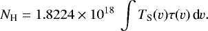
With the H I data from the H I/OH/Recombination line survey of the inner Milky Way (THOR, Beuther et al. 2016; Wang et al. 2020), we estimated the H I column density using (e.g., Wilson et al. 2013):
 (1)
(1)
The optical depth corrected spin temperature is TS(v) = TB(v)∕(1 −e−τ(v)), where TB is the brightness temperature of the H I emission. The optical depth data from Wang et al. (2020) is used to correct for the spin temperature channel by channel. We further followed the method described in Bihr et al. (2015) and corrected the column density for diffuse continuum absorption using the THOR+VGPS3 1.4 GHz continuum data (C+D+single dish GBT, see Wang et al. 2018). The derived H I column map integrated in the velocity range vLSR = 60–120 km s−1 is shown in the top-left panel of Fig. 3.
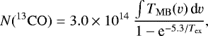
The 13CO(1–0) and 12CO(1–0) data used to characterize the molecular gas content properties are from the Galactic Ring Survey (GRS, Jackson et al. 2006) and the FOREST unbiased Galactic plane imaging survey conducted with the Nobeyama 45 m telescope (FUGIN, Umemoto et al. 2017), respectively. Assuming optically thin emission, we estimated the column density of the 13CO molecule with the equation (Wilson et al. 2013):
 (2)
(2)
where  is the column density of the 13CO molecule in cm−2, d v is the velocity in km s−1, TMB is the main beam brightness temperature in K, and Tex is the excitation temperature in K. Assuming that 12CO and 13CO share the same excitation temperatures and the 12CO line is optically thick, we can estimate Tex following the formula (Wilson et al. 2013):
 (3)
(3)
where  is the main-beam brightness temperature of the 12CO(1–0) line. The Tex were calculated for regions where
  is above the 5σ level (2 K), which results in a Tex between ~5 and 45 K. For regions where
  is below the 5σ level (2 K), an upper limit of 5 K for Tex is applied. For the galactocentric distance of 4.6 kpc of W43, the fractional abundance of 13CO relative to H2 is estimated to be 4.3 × 10⁻⁶ following the relations reported by Giannetti et al. (2014). We converted
  to N(H2) with this abundance.
Since 13CO does not trace the diffuse molecular gas (Roman-Duval et al. 2016), we used the FUGIN 12CO data (Umemoto et al. 2017) to derive the column density map of the diffuse gas. Assuming optically thin emission, we followed the standard method described in Feng et al. (2016) and derived an H2 column density map from 12CO with the same excitation temperature and 12CO abundance mentioned earlier. We then used the H2 column densities derived from 12CO instead of the column densities derived from 13CO, where the latter is 3σ lower than the former. The combined N(H2) map (vLSR = 60–120 km s−1) is shown in the top-right panel of Fig. 3. Compared to the N(H2) map derived with only 13CO emission, the combined N(H2) map has a molecular gas mass that is 56% larger.
We smoothed both the N(H) and N(H2) column density map to the same spatialresolution (46′′) and combined them to make the total gas column density map in units of hydrogen atoms cm−2 shown in the bottom panel of Fig. 3.
The total gas mass in the γ-ray emission region is 3.5 × 10⁶ M⊙. Assuming spherical geometry of the γ-ray emission region, its radius is estimated as r = d × θ ~ 5500 pc × (0.6° × π∕180°) rad ~ 60 pc. Thus the average gas number density over the volume is about 140 cm−3.
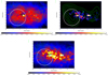 |
Fig. 3 Maps of the H I (top-left), H2 (top-right), and total (bottom) gas columns. The labels are the same as in Fig. 1. The green contours represent the γ-ray emission, the contour levels are the counts per pixel of 0.5, 0.75, 1.0, 1.25, and 1.5 in the residual map above 10 GeV (Fig. 1). The color bars represent the gas column density in cm−2. For details, see the context in Sect. 3. |
4 Discussions
4.1 Different sources in the region
There are three pulsars in the disk region from the ANTF pulsar catalog4 (Manchester et al. 2005). They are PSR J1847-0130, PSR J1848-0055, and PSR B1845-01. Their spin-down luminosities are 1.7 × 1032, 2.6 × 1033, and 7.2 × 1032 ergs s−1, while their distances are 5.8, 7.4, and 4.4 kpc, respectively. We cannot rule out the possibility that these extended γ-ray emissions are indeed PWNs, but there are no pulsars in this region that have enough spin-down power to provide the 3 × 1035 erg s−1 γ-ray luminosity, which makes this scenario quite unlikely.
There are also several SNRs near this region, including SNR G31.5-0.6 which is located inside the γ-ray emission region. The SNR G31.5-0.6 is an SNR with an incomplete shell and whose distance was estimated to be 12.9 kpc by using the Σ−D relation (Case & Bhattacharya 1998).
The mixed-morphology SNR 3C 391 is also to the east of the γ-ray emission region. It is a mid-aged SNR with an age of about 4000 yr and a distance of 7.2 kpc. The GeV emissions from this source are studied in detail in Ergin et al. (2014). It is possible that the extended γ-rays in the W43 region are produced by the interaction of ambient gas with the CRs that escaped from these SNRs.
Furthermore, the star forming region W43 is another natural acceleration site of the CRs. Indeed, the spectral shape and spatial extension are similar to those measured in other massive star clusters, such as Westerlund 2 (Yang et al. 2018), NGC 3603 (Yang & Aharonian 2017), and the Cygnus cocoon (Ackermann et al. 2011; Aharonian et al. 2019). The center of W43-main also harbors a Wolf-Rayet/O-star cluster (Blum et al. 1999). Thus the CRs accelerated by this cluster interacting with ambient gas provides a natural explanation of the extended γ-ray emissions.
4.2 Origin of the extended γ-ray emissions
As calculated in the last section, the average number density of the target protons is ~ 140 cm−3. In such dense regions, the pion-decay γ-rays will dominate the leptonic γ-rays if we assume a reasonable e/p ratio (Gabici et al. 2007). The leptonic origin of γ-rays is still feasible in the PWN scenario but, as mentioned above, it is quite unlikely due to the limited power of the pulsars in the vicinity. Thus in the discussion below we assume the γ-rays are produced in the pion-decay process from the interaction of CRs with ambient gas. To provide the γ-ray luminosity of (2.8 ± 0.4) × 1035 erg s−1, the required total CR energy would be ~2.3 ± 0.3 × 1048 erg (above 10 GeV), which is orders of magnitude smaller than those in other similar systems (Aharonian et al. 2019). However, the derived CR density is still significantly larger than densities measured in the solar neighborhood. In Fig. 2 we plot the predicted γ-ray flux assuming the CR density in W43 is the same as the local measurement.
As calculated in Yang et al. (2016) and Acero et al. (2016), the CR densities do reveal an enhancement and spectral hardening in the inner Galaxy. We thus compared the γ-ray emission we derived here with the average γ-ray spectrum in the 4–6 kpc ring in our Galaxy (the data points are from Yang et al. 2016). The results are shown in Fig. 4. The γ-ray spectrum from W43 is similar to that derived for the 4–6 kpc rings, but the total normalization is 40% smaller. Indeed, as mentioned in Aharonian et al. (2020), the enhancement of CR density in the 4-6 kpc ring is not the global variation of the level of the CR sea. Instead, the enhancement is caused by the fact that most of the active star-forming regions and, therefore, the potential particle accelerators, are located within the 4–6 kpc ring. These accelerators can create the CR-enhanced region in their vicinity. Since the CR density in such regions depends on the strength and the age of the accelerator, the densities can differ from one region to another. Thus it is not surprising that the CR density in W43 is lower than the average for the 4–6 kpc ring.
As mentioned in Aharonian et al. (2019), the CR density distribution around several massive star clusters reveals a unique 1/r profile. We perform a similar analysis for W43 to derive the CR spatial distribution.
To do this, rather than divide the γ-ray emission region into rings as in Aharonian et al. (2019), we divided it into four disk templates, as shown in Fig. 5. This is because the pote- ntial accelerator, the massive star cluster inside W43-main, is far from the center of the γ-ray emission region. We also derived the CR density in the two weak sources S1 and S2. The derived photon indices between 10 GeV and 300 GeV are 2.0 ± 0.2, 2.4 ± 0.3, 2.2 ± 0.2, and 2.3 ± 0.2. We found no significant spectral change in any of these regions, which further supports the idea that the extended emissions are of the same origin. We then performed a likelihood analysis and derived the γ-ray flux in each disk template. We then divided the γ-ray flux by the total hydrogen atom numbers derived from the mass to get the γ-ray emissivity per H atom, which is proportional to CR density. The derived CR profile is shown in the left-hand panel of Fig. 6. We also performed a jackknife test by slightly changing the position and size of these disk templates (by 0.1 degree). We found the results to be stable and the resulted differences are included in the error bars of the fluxes. We found no 1/r dependence in this case and the CR density near W43-main is significantly lower than in other parts. One explanation for such a profile is that the CRs are not accelerated exclusively in the star cluster in W43-main. Other sources, such as SNRs and other massive star clusters, reside in the W43 complex and may be also responsible for the acceleration of the CRs. We cannot exclude the possibility that these potential accelerators have not been observed in other wavebands, especially considering the very high column density and extinction toward W43. The massive stars may be invisible in the optical band due to high extinction. Ongoing near infrared surveys such as APOGEE (Roman-Lopes et al. 2018) have the ability to find these obscured massive stars in dense clouds, which may play an important role in determining the origin ofCRs in such a system. If there are multiple sources, no CR spatial distribution can be ruled out. But it is also possiblethat the CRs are dominantly contributed by another single source. To check this possibility, we also plotted the CR distribution with respect to SNR G31.5-0.6 and SNR 3C 391, which are located to the lower-left (southeast) and left (east) of the γ-ray emission regions (see Fig. 5). The profiles of the γ-ray emissivities are also shown in Fig. 6. In the case of 3C 391, we find no dependence, while in the case of SNR G31.5-0.6 the distribution reveals a clear 1/r profile. The χ2 /d.o.f. for the 1/r profile is 5.6/5, while for a uniform profile it is 16.5/5. We note that the S2 position coincides with SNR G29.7-0.3/HESS J1846-029/PSR J1846-0258. It is possible that S2 is the low energy counterpart of the TeV source HESS J1846-029. Thus we also estimated the profile by ignoring S1 and S2. In this case, the χ2 ∕d.o.f. is 2.5/3 for a 1/r profile, and 13.3/3 for a uniform profile. The distance of SNR G31.5-0.6 was estimated to be 12.9 kpc, using the Σ−D relation (Case & Bhattacharya 1998). If this is true, SNR G31.5-0.6 can hardly be responsible for the CRs illuminating W43 region. But it is also possible that SNR G31.5-0.6 does not obey the Σ−D relation used in deriving the distance. In this case, SNR G31.5-0.6 can also be regarded as a potential accelerator of CRs in this region.
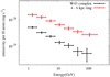 |
Fig. 4 The γ-ray SEDs of W43-main and in the 4-6 kpc ring from Yang et al. (2016). |
4.3 Acceleration mechanisms
Recently, Aharonian et al. (2019) proposed that young star clusters can be an alternative source population of Galactic CRs, and that the γ-ray emissions around such objects can be a powerful tool to diagnose the acceleration of CRs and the propagationof CRs in the vicinity of sources. Several such systems have already been detected in the γ-ray band, such as the Cygnus cocoon (Ackermann et al. 2011; Aharonian et al. 2019), Westerlund 1 (Abramowski et al. 2012), Westerlund 2 (Yang et al. 2018), NGC 3603 (Yang & Aharonian 2017), and 30 Dor C (H.E.S.S. Collaboration 2015). Here, we report a statistically significant detection of an extended γ-ray signal from the direction of another young star forming region, W43. Like in the other systems, the spectrum of this source is harder than the local CR spectra. We argue that the most likely origin of the detected emission is the interactions of CRs with the surrounding gas, which are accelerated in the star forming region.
However, the exact CR accelerator is not clear at this moment. The most natural source, the massive star cluster in W43-main, is likely not the source according to the CR density profile. A source located to the southeast of W43 can recover a 1/r profile observed in other similar systems. We note that the 1/r profile implies a continuous injection of CRs. Thus the size of the γ-ray emission region can be used to constrain the age of the accelerator. If we attribute the farthest γ-ray emission S2 to be related to the source, the size l of the γ-ray emission region is larger than 150 pc. Thus the age should be larger than T =l2∕2D. If we take the standard diffusion coefficient in the Galactic plane of 1028 cm2 s−1 into account, the derived age is larger than 105 yr, which seems too long for an SNR and also favors a massive star cluster scenario of CR accelerations. We note that it is quite common for OB starsto be missed in such a dense region; the APOGEE survey has revealed four times more OB stars than identified before in the W345 complex (Roman-Lopes et al. 2019). Such dedicated near infrared surveys will shed light on the origin of these diffuse γ-ray emissions and play an important role in the study of the CR origin in our Galaxy.
Another interesting issue is that the γ-ray luminosity is proportional to the SFR in starburst galaxies (Ackermann et al. 2012). The natural explanation is that those galaxies are CR calorimeters and the γ-ray luminosity is the same as the CR injection rate. Thus the aforementioned relationship indicates that the CR injection rate depends on the SFR.
To extend the study to nearby Galactic systems, we included another two γ-ray detected Galactic star forming (starburst) regions: the Cygnus cocoon (powered by Cygnus OB2) (Ackermann et al. 2011; Aharonian et al. 2019) and NGC 3603 (Yang & Aharonian 2017). However, due to the compact size, most of the accelerated CRs will escape the source region before losing their energies. Thus, rather than compare the γ-ray luminosities, we calculated the total CR energies from the γ-ray observations and the gas distributions. As derived in Sect. 3, the total CR energy in W43 is (2.3 ± 0.3) × 1048 erg. The total CR energy in NGC 3603 and the Cygnus cocoon are (7.5 ± 2.5) × 1049 erg (Yang & Aharonian 2017) and (1.0 ± 0.2) × 1049 erg (Aharonian et al. 2019), respectively. However, as mentioned in Aharonian et al. (2019), the total CR energy estimated from γ-ray emission may be biased due to the fact that the CRs may occupy a much larger volume but cannot be traced by γ-rays due to the low gas density therein. Of these three cases, the γ-ray emission region of NGC 3603 is much more extended than the other two. Thus, to make the comparison feasible, we normalized the CR density to the same volume by assuming a 1/r distribution of CR density, although we did not find such a relationship in W43.
Nguyen-Luong et al. (2016) derived the immediate past SFR from the radio continuum for the Cygnus X region (which includes Cygnus OB2) and W43. We estimated the average SFR of NGC 3603 by simply dividing the mass of a cluster by its age (Beccari et al. 2010). We find that although W43 has much larger SFRs than the other two, the injected CR energy is much lower, which is contrary to the relationship found in galaxies.
We further investigated the relationship between CR energy and wind power in these regions. As estimated in Domingo-Santamaría & Torres (2006), the wind power of a single Wolf-Rayet star or early type-O star can be as large as 1037 erg s−1, while for B-stars the value drops by orders of magnitude. Thus, the wind power in these regions should be dominated by O-stars and Wolf-Rayet stars. Cygnus OB2 and NGC 3603 both contain several dozen O-stars. Ackermann et al. (2011) estimated the total wind power of Cygnus OB2 to be 2−3 × 1038 erg s−1. Wright et al. (2010) mentioned that the number of O-stars in NGC 3603 is about two-thirds of that in Cygnus OB2. Thus we simply estimated the total wind power in NGC3603 to also be two-thirds of that in Cygnus OB2. We note that this estimation is quite conservative since although there are fewer O-stars in NGC 3603, four of them have already been identified as Wolf-Rayet stars (Harayama et al. 2008). For W43, so far only one Wolf-Rayet and two O-stars have been identified (Blum et al. 1999). Thus we estimated the wind power to be about 3 × 1037 erg s−1. The physical properties of all three regions are listed in Table 2. In this case we found a clear correlation between the wind power and total CR energy. We regarded it as an indication that in such systems CRs are indeed accelerated by star winds.
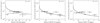 |
Fig. 6 The γ-ray emissivity per H atom with respect to W43-main (left panel), SNR G31.5-0.6 (middle panel), and SNR 3C391 (right panel). The curves are the projected 1/r profile. |
Physical parameters of three extended γ-ray structures and the star forming region.
5 Conclusion
In this paper we analyze the γ-ray emission from the Galactic mini-starburst W43. We find an extended γ-ray emission with a radius of 0.6° and a significance of 16 σ. The emission reveals a hard spectrum, with a spectral index of about 2.3. The spatial and spectral features are similar to the γ-ray emissions in other massive star clusters such as NGC 3603 (Yang & Aharonian 2017), Westerlund 2 (Yang et al. 2018), and the Cygnus cocoon (Aharonian et al. 2019). Due to the high gas density in this region, the most probable γ-ray emission mechanism is the pion-decay process that is the result of the interaction of CR protons with the ambient gas. In comparison with similar systems, we find that the total CR energy in the star forming region is better correlated with the wind power than with the SFR. We derived the CR profile in the γ-ray emission region. We find that, unlike the Cygnus cocoon and Westerlund 2, the CR distribution does not reveal a 1/r profile over the central massive star clusters. However, it is quite likely that the massive star associations/clusters were missed in former studies due to high extinction in this dense region. Dedicated near infrared surveys such as APOGEE (Roman-Lopes et al. 2018) will shed light on the origin of these diffuse γ-ray emissions and play an important role in the study of the CR origin in our Galaxy.
Acknowledgements
R.Y. is supported by the NSFC under grants 11421303 and the national youth thousand talents program in China.
References
- Abdo, A. A., Ackermann, M., Ajello, M., et al. 2009, ApJ, 706, L1 [NASA ADS] [CrossRef] [Google Scholar]
- Abramowski, A., Acero, F., Aharonian, F., et al. 2012, A&A, 537, A114 [NASA ADS] [CrossRef] [EDP Sciences] [Google Scholar]
- Acero, F., Ackermann, M., Ajello, M., et al. 2013, ApJ, 773, 77 [CrossRef] [Google Scholar]
- Acero, F., Ackermann, M., Ajello, M., et al. 2016, ApJS, 223, 26 [NASA ADS] [CrossRef] [EDP Sciences] [Google Scholar]
- Ackermann, M., Ajello, M., Allafort, A., et al. 2011, Science, 334, 1103 [NASA ADS] [CrossRef] [PubMed] [Google Scholar]
- Ackermann, M., Ajello, M., Allafort, A., et al. 2012, ApJ, 755, 164 [NASA ADS] [CrossRef] [Google Scholar]
- Aharonian, F., Yang, R., & de Oña Wilhelmi, E. 2019, Nat. Astron., 3, 561 [NASA ADS] [CrossRef] [Google Scholar]
- Aharonian, F., Peron, G., Yang, R., Casanova, S., & Zanin, R. 2020, Phys. Rev. D 101, 083018 [NASA ADS] [CrossRef] [Google Scholar]
- Beccari, G., Spezzi, L., De Marchi, G., et al. 2010, ApJ, 720, 1108 [NASA ADS] [CrossRef] [Google Scholar]
- Beuther, H., Bihr, S., Rugel, M., et al. 2016, A&A, 595, A32 [NASA ADS] [CrossRef] [EDP Sciences] [Google Scholar]
- Bihr, S., Beuther, H., Ott, J., et al. 2015, A&A, 580, A112 [NASA ADS] [CrossRef] [EDP Sciences] [Google Scholar]
- Blasi, P. 2013, A&ARv, 21, 70 [Google Scholar]
- Blum, R. D., Damineli, A., & Conti, P. S. 1999, AJ, 117, 1392 [NASA ADS] [CrossRef] [Google Scholar]
- Casandjian, J.-M. 2015, ArXiv e-prints [arXiv:1502.07210] [Google Scholar]
- Case, G. L., & Bhattacharya, D. 1998, ApJ, 504, 761 [Google Scholar]
- Domingo-Santamaría, E., & Torres, D. F. 2006, A&A, 448, 613 [NASA ADS] [CrossRef] [EDP Sciences] [Google Scholar]
- Ergin, T., Sezer, A., Saha, L., et al. 2014, ApJ, 790, 65 [NASA ADS] [CrossRef] [Google Scholar]
- Feng, S., Beuther, H., Zhang, Q., et al. 2016, A&A, 592, A21 [NASA ADS] [CrossRef] [EDP Sciences] [Google Scholar]
- Gabici, S., Aharonian, F. A., & Blasi, P. 2007, Ap&SS, 309, 365 [CrossRef] [Google Scholar]
- Giannetti, A., Wyrowski, F., Brand, J., et al. 2014, A&A, 570, A65 [NASA ADS] [CrossRef] [EDP Sciences] [Google Scholar]
- Harayama, Y., Eisenhauer, F., & Martins, F. 2008, ApJ, 675, 1319 [NASA ADS] [CrossRef] [Google Scholar]
- H.E.S.S. Collaboration (Abramowski, A., et al.) 2015, Science, 347, 406 [NASA ADS] [CrossRef] [Google Scholar]
- H.E.S.S. Collaboration (Abdalla, H., et al.) 2018, A&A, 612, A1 [NASA ADS] [CrossRef] [EDP Sciences] [Google Scholar]
- Jackson, J. M., Rathborne, J. M., Shah, R. Y., et al. 2006, ApJS, 163, 145 [NASA ADS] [CrossRef] [Google Scholar]
- Lande, J., Ackermann, M., Allafort, A., et al. 2012, ApJ, 756, 5 [NASA ADS] [CrossRef] [Google Scholar]
- Manchester, R. N., Hobbs, G. B., Teoh, A., & Hobbs, M. 2005, AJ, 129, 1993 [NASA ADS] [CrossRef] [Google Scholar]
- Motte, F., Schilke, P., & Lis, D. C. 2003, ApJ, 582, 277 [NASA ADS] [CrossRef] [Google Scholar]
- Nguyen Luong, Q., Motte, F., Schuller, F., et al. 2011, A&A, 529, A41 [NASA ADS] [CrossRef] [EDP Sciences] [Google Scholar]
- Nguyen-Luong, Q., Nguyen, H. V. V., Motte, F., et al. 2016, ApJ, 833, 23 [NASA ADS] [CrossRef] [Google Scholar]
- Papadopoulos,P. P. 2010, ApJ, 720, 226 [NASA ADS] [CrossRef] [Google Scholar]
- Roman-Duval,J., Heyer, M., Brunt, C. M., et al. 2016, ApJ, 818, 144 [NASA ADS] [CrossRef] [Google Scholar]
- Roman-Lopes,A., Román-Zúñiga, C., Tapia, M., et al. 2018, ApJ, 855, 68 [CrossRef] [Google Scholar]
- Roman-Lopes, A., Román-Zúñiga, C. G., Tapia, M., et al. 2019, ApJ, 873, 66 [Google Scholar]
- Stil, J. M., Taylor, A. R., Dickey, J. M., et al. 2006, AJ, 132, 1158 [NASA ADS] [CrossRef] [Google Scholar]
- The Fermi-LAT Collaboration 2020, ApJS, 247, 33 [NASA ADS] [CrossRef] [Google Scholar]
- Umemoto, T., Minamidani, T., Kuno, N., et al. 2017, PASJ, 69, 78 [NASA ADS] [CrossRef] [Google Scholar]
- Wang, Y., Bihr, S., Rugel, M., et al. 2018, A&A, 619, A124 [NASA ADS] [CrossRef] [EDP Sciences] [Google Scholar]
- Wang, Y., Beuther, H., Rugel, M. R., et al. 2020, A&A, 634, A83 [NASA ADS] [CrossRef] [EDP Sciences] [Google Scholar]
- Wilson, T. L., Rohlfs, K., & Hüttemeister, S. 2013, Tools of Radio Astronomy (Berlin: Springer) [CrossRef] [Google Scholar]
- Wright, N. J., Drake, J. J., Drew, J. E., & Vink, J. S. 2010, ApJ, 713, 871 [NASA ADS] [CrossRef] [Google Scholar]
- Yang, R.-z., & Aharonian, F. 2017, A&A, 600, A107 [NASA ADS] [CrossRef] [EDP Sciences] [Google Scholar]
- Yang, R., Aharonian, F., & Evoli, C. 2016, Phys. Rev. D, 93, 123007 [Google Scholar]
- Yang, R.-z., de Oña Wilhelmi, E., & Aharonian, F. 2018, A&A, 611, A77 [NASA ADS] [CrossRef] [EDP Sciences] [Google Scholar]
- Zhang, B., Moscadelli, L., Sato, M., et al. 2014, ApJ, 781, 89 [NASA ADS] [CrossRef] [Google Scholar]
The Very Large Array Galactic Plane Survey, Stil et al. (2006).
All Tables
Physical parameters of three extended γ-ray structures and the star forming region.
All Figures
|
Fig. 1 The residual counts map above 10 GeV in the 5° × 5° region near W43, with pixel size of 0.1° × 0.1°, smoothed with a Gaussian filter of 0.2°. The color bars represent the counts per pixel. The white circle is the best-fit uniform disk template. The small black circle marks the position of the star forming region W43-main. The cyan diamonds are the weak sources S1 and S2. The green crosses indicate the point sources listed in the 4FGL. The magenta circle marks the position and size of the TeV source HESS J1848-018. The two black crosses mark the position of the two HESS point sources, HESS J1846-029 (left) and HESS J1844-030 (right), respectively. The white boxes are the positions of the nearby SNRs. |
| In the text | |
|
Fig. 2 The SED of γ-ray emission toward W43 for a uniform disk spatial model with a radius of 0.6°, normalized to emissivity per H atom. The distance of 5.5 kpc is used and the masses are derived in Sect. 3. The solid curve represents the spectrum of emissivity per H atom, assuming the energy distribution of protons is the same as the local intestellar spectrum (LIS) (Casandjian 2015). Also plotted are the normalized SEDs of the Cygnus cocoon (Aharonian et al. 2019) and NGC 3603 (Yang & Aharonian 2017). |
| In the text | |
|
Fig. 3 Maps of the H I (top-left), H2 (top-right), and total (bottom) gas columns. The labels are the same as in Fig. 1. The green contours represent the γ-ray emission, the contour levels are the counts per pixel of 0.5, 0.75, 1.0, 1.25, and 1.5 in the residual map above 10 GeV (Fig. 1). The color bars represent the gas column density in cm−2. For details, see the context in Sect. 3. |
| In the text | |
|
Fig. 4 The γ-ray SEDs of W43-main and in the 4-6 kpc ring from Yang et al. (2016). |
| In the text | |
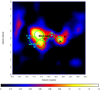 |
Fig. 5 The same as Fig. 1 but overlaid with the disk region we used to extract the CR profile. |
| In the text | |
|
Fig. 6 The γ-ray emissivity per H atom with respect to W43-main (left panel), SNR G31.5-0.6 (middle panel), and SNR 3C391 (right panel). The curves are the projected 1/r profile. |
| In the text | |
Current usage metrics show cumulative count of Article Views (full-text article views including HTML views, PDF and ePub downloads, according to the available data) and Abstracts Views on Vision4Press platform.
Data correspond to usage on the plateform after 2015. The current usage metrics is available 48-96 hours after online publication and is updated daily on week days.
Initial download of the metrics may take a while.