| Issue |
A&A
Volume 639, July 2020
|
|
|---|---|---|
| Article Number | A55 | |
| Number of page(s) | 4 | |
| Section | Galactic structure, stellar clusters and populations | |
| DOI | https://doi.org/10.1051/0004-6361/202038239 | |
| Published online | 07 July 2020 | |
Binary star sequence in the outskirts of the disrupting Galactic open cluster UBC 274
1
Instituto Interdisciplinario de Ciencias Básicas (ICB), CONICET UNCUYO, Padre J. Contreras 1300, M5502JMA Mendoza, Argentina
e-mail: This email address is being protected from spambots. You need JavaScript enabled to view it.
2
Consejo Nacional de Investigaciones Científicas y Técnicas (CONICET), Godoy Cruz 2290, C1425FQB Buenos Aires, Argentina
Received:
23
April
2020
Accepted:
6
June
2020
Abstract
We report the identification of a numerous binary star population in the recently discovered ∼3 Gyr old open cluster UBC 274. It becomes visible when the cluster color-magnitude diagram is corrected by differential reddening and spans mass ratio (q) values from 0.5 up to 1.0. Its stellar density radial profile and cumulative distribution as a function of the distance from the cluster center reveal that it extends out to the observed boundaries of the tidal tails of the cluster (about six times the cluster radius) following a spatial distribution indistinguishable from that of cluster main-sequence (MS) stars. Furthermore, binary stars with q values lower or higher than 0.75 do not show any spatial distribution difference either. From Gaia DR2 astrometric and kinematics data we computed Galactic coordinates and space velocities with respect to the cluster center and mean cluster space velocity, respectively. We found that cluster members located throughout the tidal tails move relatively fast, regardless of whether they are a single or binary star. The projection of their motions onto the Galactic plane resembles that of a rotating solid body, while the motions along the radial direction from the Galactic center and perpendicular to the Galactic plane suggest that the cluster is being disrupted. The similarity of the spatial distributions and kinematic patterns of cluster MS and binary stars reveals that UBC 274 is facing an intense process of disruption that has apparently swept out any signature of internal dynamic evolution, such as mass segregation driven by two-body relaxation.
Key words: open clusters and associations: general / open clusters and associations: individual: UBC 274 / techniques: photometric
© ESO 2020
1. Introduction
The source UBC 274 (RA: 10h24m46.50s, Dec: −72°34′28.36″, l: 292°. 3622, b: −12 7920) is a Galactic open cluster that has recently been discovered by Castro-Ginard et al. (2020) in astrometric, kinematics, and photometric data sets available at the Gaia DR2 archive1 (Gaia Collaboration 2016, 2018b,a). The authors recognized the new object after applying a technique based on machine-learning and a deep-learning artificial neural network. The source is a ∼3 Gyr old open cluster (see the cluster color-magnitude diagram (CMD) built by them in Fig. 1) located at ∼2 kpc from the Sun. Based on a comparison with 365 bona fide members, the authors found that the cluster has a remarkably elongated shape, from which they concluded that it is subjected to an extensive tidal disruption process.
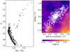 |
Fig. 1. Observed cluster CMD (left panel). Interstellar reddening (E(B − V)) map for the cluster field (right panel). The cluster members are represented by open circles whose sizes are proportional to their G brightnesses. |
Because of its populous extra-tidal features, the cluster deserves much more of our attention. For instance, an analysis of the spatial distribution of the different stellar populations in the cluster CMD would contribute to determining its ongoing internal dynamical evolutionary stage (see, e.g., Angelo et al. 2019; Piatti et al. 2019a). The relatively deep and complete cluster CMD might also be useful to dive into the still-debated existence of extended main-sequence (MS) turnoffs in Galactic open clusters and their origin (see, e.g., Cordoni et al. 2018; Piatti & Bonatto 2019; de Juan Ovelar et al. 2020). The position and shape of the observed tidal tails might be used to constrain models of the formation of substructures along them (see, e.g., Montuori et al. 2007; Küpper et al. 2010), among others.
In this work, we closely revisit the Gaia DR2 data set for the 365 cluster members identified by Castro-Ginard et al. (2020). We find that UBC 274 contains a well-populated binary sequence that extends out to the observed outskirts of the disrupting cluster, following similar spatial and kinematical distributions as escaping single-cluster MS stars. If the internal dynamics of UBC 274 were driven by two-body relaxation alone, its binary population should be more centrally concentrated than that of the single stars. To our knowledge, we report the first open cluster without different spatial distributions of single and binary stars. The analysis is organized as follows: in Sect. 2 we present an intrinsic cluster CMD from which we identify the cluster binary star population, while in Sect. 3 we discuss its resulting spatial and kinematical distributions. Finally, in Sect. 4 we summarize the main outcomes of this work.
2. Cluster binary star sequence
Differential reddening in the field of star clusters can blur fundamental features of their CMDs. For this reason, we first examined the spatial variation of the interstellar reddening across UBC 274. We built the interstellar reddening map by retrieving the E(B − V) values obtained by Schlafly & Finkbeiner (2011) and provided by NASA/IPAC Infrared Science Archive2. Figure 1 depicts the resulting spatial distribution of E(B − V) values, where we superimposed the loci of cluster members, represented by open circles with sizes proportional to their G brightnesses. The cluster field is affected by some amount of differential reddening. We then corrected the G magnitude and GBP − GRP color of each star for interstellar reddening using the corresponding individual E(B − V) value according to the stellar coordinates in the reddening map and the relationships AG = 2.44E(B − V) and E(GBP − GRP) = 1.27E(B − V) (Cardelli et al. 1989; Wang & Chen 2019). Figure 2 shows the reddening-corrected (intrinsic) CMD.
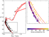 |
Fig. 2. Intrinsic cluster CMD (left panel). Isochrones of log(t/yr) = 9.45 (solid line), 9.40, and 9.50 (dotted lines) are superimposed. The rectangle illustrates the zoom-in region depicted in the right panel, where the isochrone of log(t/yr) = 9.45 is superimposed for q = 0, 0.5, and 1.0 with solid, dotted, and dashed lines, respectively. |
The observed cluster CMD clearly shows a red giant branch, a red clump, a subgiant branch, a nearly 4 mag long MS, and a binary star sequence spanning the whole MS magnitude range. After the reddening correction, the binary star sequence is much more pronounced. Hence, we emphasize in the importance of correcting the Gaia DR2 photometry for differential reddening as a crucial step to make the well-delineated and populous cluster binary star strip visible. Then, we adopted the mean cluster parallax and the cluster metallicity from Castro-Ginard et al. (2020) and found that the Bressan et al. (2012) theoretical isochrone that resembles the cluster features best, that is, position and shape of the different giant phases, the MS turnoff and the curvature of the MS, is that of log(t/yr) = 9.45 ± 0.05 (2.8 ± 0.2 Gyr) (see Fig. 2, left panel).
We statistically distinguished the cluster binary star population from the cluster MS by running extensive Monte Carlo experiments. We considered the photometric errors in G and GBP − GRP derived by Evans et al. (2018) and the errors in E(B − V) from Schlafly & Finkbeiner (2011), and used the isochrone of log(t/yr) = 9.45 as a ridge line for the cluster MS from G0 = 14.3 mag down to 16.8 mag (see Fig. 2, right panel). In order to estimate the probability for a star to belong to the cluster MS, we measured the distance from that star to the cluster ridge line, adopting for both end points (the star and the closest position on the cluster ridge line) the corresponding errors in G0 and (GBP − GRP)0. We performed 1000 measurements of this distance, allowing random values of magnitudes and colors within 3σ for the star and the position on the ridge line, respectively. Then, we considered that a star belongs to the cluster MS if it meets the criterion that the distance to the MS is shorter than the sum of the errors along the line connecting the star and the ridge line. We finally obtained the probability (P) of a star to belong to the cluster MS by dividing by 10 the number of times it satisfied the above criterion. The difference 100–P gives the probability of a star to be a binary star. This is because all the stars are assumed to be cluster members according to the membership criteria applied by Castro-Ginard et al. (2020). Figure 2 (right panel) shows color-coded binary probabilities. In the subsequent analysis we consider as binary stars those with P < 40%, which roughly corresponds to secondary-to-primary mass ratios M2/M1 = q ≳ 0.5.
3. Analysis and discussion
Using the positions of cluster MS and binary stars, we constructed their respective radial density profiles by counting the stars that are distributed throughout the cluster region (see Fig. 1). First, we split the cluster area into small adjacent boxes of  that covered the entire analyzed field. Then, we counted the number of stars (MS and binary stars separately) inside them and computed the mean densities as a function of the distance to the cluster center (d) by averaging the star counts in every box placed within the annulus centered on the cluster with radii d and d + Δd). This allowed us to estimate the uncertainties in star counts due to stellar fluctuations within each annulus. We repeated this method using boxes of increasing size in steps of
  per side, up to
  . The resulting radial density profiles shown in Fig. 3 (left panel) were obtained by averaging all the generated individual density radial profiles. We also built cumulative distributions as a function of d (see Fig. 3, right panel) where the errors were calculated according to the Poisson statistics. For comparison purposes, we also constructed the above curves for cluster red giant stars (G0 < 13.8 mag, (GBP − GRP)0> 1.0 mag), although this is hampered by small number statistics.
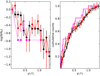 |
Fig. 3. Observed radial density profiles (left panel) and cumulative distribution functions (right panel) for cluster MS (black lines), binary (red lines), and red giant stars (magenta lines). Error bars are also indicated. |
Figure 3 reveals that cluster MS and binary stars are distributed following an indistinguishable spatial pattern, from the cluster core region out to the observed boundaries of its tidal tails ( from the cluster center). To our knowledge, binary stars populating cluster tidal tail regions out to about six times the cluster radius (
 for UBC 274) have not been observed in any Galactic open cluster before. Here we estimated the radius of the cluster main body as the distance r with the highest density contrast, calculated as the ratio between the number of stars inside r to the number of stars in an annulus of interior radius r and equal area. We refer to some detailed studies of open clusters with well-known tidal tails: Hyades (Röser et al. 2019), Praesepe (Röser & Schilbach 2019), Coma Berenices (Tang et al. 2019), and Blanco 1(Zhang et al. 2020), among others. Furthermore, cluster binary stars have so far been observed to be more centrally concentrated than single MS stars because of mass segregation that is caused by the dynamics internal evolution driven by two-body relaxation (Reino et al. 2018; Gao 2018; Cohen et al. 2020), even though open clusters have also been subject of tidal effects due to the gravitational potential of the Milky Way (Piatti & Mackey 2018; Piatti et al. 2019b). We therefore conclude that UBC 274 has become the first open cluster that has a numerous binary star population with a unique density profile. The radial and cumulative density profiles of red giant stars also indicate that the signatures of the internal cluster dynamical evolution are removed. This conjecture is affected by small number statistics, however.
We further investigated the spatial distribution of the ratio between the mass of the primary (M1) and that of the secondary (M2) binary star (M2/M1 = q, 0 ≤ q ≤ 1). Following the precepts outlined by Hurley & Tout (1998) and using the theoretical isochrone of log(t/yr) = 9.45 (Bressan et al. 2012), we computed the G0 magnitudes for binary stars with q values from 0.5 up to 1.0 in steps of 0.1 (see Fig. 2, right panel). We then interpolated the CMD positions of the binary stars in the different generated binary star sequences in order to assign them the corresponding q values. Figure 4 (left panel) shows the distribution of q values as a function of d and G0 magnitudes. More massive binary stars (smaller G0 magnitudes) are found to be distributed along the entire d range, regardless of their q values. This trend is confirmed by the cumulative distribution functions built using binary stars with q values lower or higher than 0.75 (see Fig. 4, right panel). Moreover, the two binary star groups also seem to share similar density profiles.
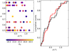 |
Fig. 4. q values associated with the cluster binary stars as a function of d, color-coded according to their intrinsic G0 magnitudes (left panel). The cumulative distribution for binary stars with q values lower or higher than 0.75 are depicted with a red and black line, respectively (right panel). |
We finally analyzed the kinematics of cluster MS and binary stars from the Gaia DR2 coordinates, proper motions, parallaxes, and radial velocities. Radial velocities are available for 13 cluster members. For cluster members without RV measurements, we assigned values that were randomly generated in the range [⟨RV⟩ − σ(RV),⟨RV⟩ + σ(RV)], where ⟨RV⟩ and σRV are the cluster mean value and dispersion obtained by Castro-Ginard et al. (2020). We computed Galactic coordinates (X, Y, Z) and space velocities (VX, VY, VZ) employing the astropy3 package (Astropy Collaboration 2013, 2018), which simply required the input of the astrometric and kinematic data mentioned above. Figure 5 illustrates the space velocity vector field with respect to the mean cluster motion projected on different Galactic planes (coordinates relative to the cluster center). The figure reveals that both cluster MS and binary stars are moving remarkably fast with respect to the cluster center throughout the tidal tails. In order to better understand this velocity pattern, we plot in Fig. 6 the spherical components of the space velocities of the stars with respect to the mean cluster velocity as a function of the relative Galactocentric distances of them with respect to the that of the cluster center. From a kinematical point of view, Fig. 6 provides further support that cluster MS and binary stars that are located at any position of the cluster main body or tidal tails have similar kinematical behaviors. Additionally, the figure shows that while the projection of the cluster motion on the plane of the Galactic disk rotates like a solid body (bottom panel), the cluster is being disrupted along the direction from the Galactic center (top panel) and along the direction perpendicular to the Galactic plane (middle panel).
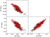 |
Fig. 5. Space velocity vectors with respect to the mean cluster motion projected on different Galactic planes (relative XYZ coordinates) for cluster MS and binary stars, represented by black and red arrows, respectively. |
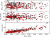 |
Fig. 6. Difference between individual space velocity components and those of the mean cluster space velocity (spherical coordinate framework) as a function of RGC (relative values). |
4. Conclusions
Motivated by the recent discovery of UBC 274, an ∼3 Gyr old open cluster located at ∼2 kpc from the Sun, which exhibits extended tidal tails, we revisited the Gaia DR2 data set for 365 cluster members. In the cluster CMD corrected for differential reddening, we recognized a numerous binary star population that is distributed throughout the whole magnitude dynamical range of the cluster MS and toward redder colors. This binary star population spans q values from 0.5 up to 1.0, which we obtained by interpolation in a set of generated binary star sequences from the theoretical isochrone computed by Bressan et al. (2012) for the cluster age. We point out that the binary star strip is neither recognized from the observer cluster CMD nor from that corrected for the mean cluster reddening.
We separately built stellar density radial profiles and cumulative distribution functions from the cluster center out to about six times its radius for cluster MS and binary stars. The resulting radial profiles and cumulative distributions show that binary stars reach the outermost regions of the observed tidal tails and follow a similar spatial distribution pattern as cluster MS stars. Moreover, in terms of spatial distribution, binary stars with q values lower or higher than 0.75 do not show any difference either. The result that a relatively large number of binary stars populates the tidal tails of the cluster might become observational evidence that supports the idea that a percentage of the field binary stars comes from disrupted star clusters (Goodwin 2010).
For the kinematics of cluster members, we computed Galactic coordinates and space velocity components (Cartesian and spherical frameworks) from the available astrometric and kinematic information. We found that stars located along the tidal tails of the cluster’s tidal tails move relatively fast with respect to the cluster center, regardless of whether they are MS or binary stars. In particular, the projected stellar motions on the Galactic plane with respect to the cluster center resembles that of a rotating solid body, while the motions along the direction from the Galactic center and perpendicular to the Galactic plane suggest that the clusters is being disrupted. The resulting disrupting directions agree very well with realistic N-body simulations of the orbit of star clusters with tidal tails (e.g., Montuori et al. 2007). The similarity found in the spatial distributions and kinematic patterns of cluster MS and binary stars reveals that UBC 274 is facing an intense process of disruption that has apparently swept out any signature of internal dynamics evolution driven by two-body relaxation.
Acknowledgments
I thank the referee for the thorough reading of the manuscript and timely suggestions to improve it. I also acknowledge support from the Ministerio de Ciencia, Tecnología e Innovación Productiva (MINCyT) through grant PICT-201-0030.
References
- Angelo, M. S., Piatti, A. E., Dias, W. S., & Maia, F. F. S. 2019, MNRAS, 488, 1635 [NASA ADS] [CrossRef] [Google Scholar]
- Astropy Collaboration (Robitaille, T. P., et al.) 2013, A&A, 558, A33 [NASA ADS] [CrossRef] [EDP Sciences] [Google Scholar]
- Astropy Collaboration (Price-Whelan, A. M., et al.) 2018, AJ, 156, 123 [Google Scholar]
- Bressan, A., Marigo, P., Girardi, L., et al. 2012, MNRAS, 427, 127 [NASA ADS] [CrossRef] [Google Scholar]
- Cardelli, J. A., Clayton, G. C., & Mathis, J. S. 1989, ApJ, 345, 245 [NASA ADS] [CrossRef] [Google Scholar]
- Castro-Ginard, A., Jordi, C., Luri, X., et al. 2020, A&A, 635, A45 [NASA ADS] [CrossRef] [EDP Sciences] [Google Scholar]
- Cohen, R. E., Geller, A. M., & von Hippel, T. 2020, AJ, 159, 11 [CrossRef] [Google Scholar]
- Cordoni, G., Milone, A. P., Marino, A. F., et al. 2018, ApJ, 869, 139 [NASA ADS] [CrossRef] [Google Scholar]
- de Juan Ovelar, M., Gossage, S., Kamann, S., et al. 2020, MNRAS, 491, 2129 [Google Scholar]
- Evans, D. W., Riello, M., De Angeli, F., et al. 2018, A&A, 616, A4 [NASA ADS] [CrossRef] [EDP Sciences] [Google Scholar]
- Gaia Collaboration (Prusti, T., et al.) 2016, A&A, 595. A1 [NASA ADS] [CrossRef] [EDP Sciences] [Google Scholar]
- Gaia Collaboration (Helmi, A., et al.) 2018a, A&A, 616, A12 [NASA ADS] [CrossRef] [EDP Sciences] [Google Scholar]
- Gaia Collaboration (Brown, A. G. A., et al.) 2018b, A&A, 616, A1 [NASA ADS] [CrossRef] [EDP Sciences] [Google Scholar]
- Gao, X. 2018, ApJ, 869, 9 [NASA ADS] [CrossRef] [Google Scholar]
- Goodwin, S. P. 2010, Philos. Trans. R. Soc. London Ser. A, 368, 851 [NASA ADS] [CrossRef] [Google Scholar]
- Hurley, J., & Tout, C. A. 1998, MNRAS, 300, 977 [NASA ADS] [CrossRef] [MathSciNet] [Google Scholar]
- Küpper, A. H. W., Kroupa, P., Baumgardt, H., & Heggie, D. C. 2010, MNRAS, 401, 105 [NASA ADS] [CrossRef] [Google Scholar]
- Montuori, M., Capuzzo-Dolcetta, R., Di Matteo, P., Lepinette, A., & Miocchi, P. 2007, ApJ, 659, 1212 [NASA ADS] [CrossRef] [Google Scholar]
- Piatti, A. E., & Bonatto, C. 2019, MNRAS, 490, 2414 [Google Scholar]
- Piatti, A. E., & Mackey, A. D. 2018, MNRAS, 478, 2164 [NASA ADS] [CrossRef] [Google Scholar]
- Piatti, A. E., Angelo, M. S., & Dias, W. S. 2019a, MNRAS, 488, 4648 [NASA ADS] [CrossRef] [Google Scholar]
- Piatti, A. E., Webb, J. J., & Carlberg, R. G. 2019b, MNRAS, 489, 4367 [NASA ADS] [CrossRef] [Google Scholar]
- Reino, S., de Bruijne, J., Zari, E., d’Antona, F., & Ventura, P. 2018, MNRAS, 477, 3197 [NASA ADS] [CrossRef] [Google Scholar]
- Röser, S., & Schilbach, E. 2019, A&A, 627, A4 [NASA ADS] [CrossRef] [EDP Sciences] [Google Scholar]
- Röser, S., Schilbach, E., & Goldman, B. 2019, A&A, 621, L2 [NASA ADS] [CrossRef] [EDP Sciences] [Google Scholar]
- Schlafly, E. F., & Finkbeiner, D. P. 2011, ApJ, 737, 103 [NASA ADS] [CrossRef] [Google Scholar]
- Tang, S.-Y., Pang, X., Yuan, Z., et al. 2019, ApJ, 877, 12 [NASA ADS] [CrossRef] [Google Scholar]
- Wang, S., & Chen, X. 2019, ApJ, 877, 116 [NASA ADS] [CrossRef] [Google Scholar]
- Zhang, Y., Tang, S.-Y., Chen, W. P., Pang, X., & Liu, J. Z. 2020, ApJ, 889, 99 [CrossRef] [Google Scholar]
All Figures
|
Fig. 1. Observed cluster CMD (left panel). Interstellar reddening (E(B − V)) map for the cluster field (right panel). The cluster members are represented by open circles whose sizes are proportional to their G brightnesses. |
| In the text | |
|
Fig. 2. Intrinsic cluster CMD (left panel). Isochrones of log(t/yr) = 9.45 (solid line), 9.40, and 9.50 (dotted lines) are superimposed. The rectangle illustrates the zoom-in region depicted in the right panel, where the isochrone of log(t/yr) = 9.45 is superimposed for q = 0, 0.5, and 1.0 with solid, dotted, and dashed lines, respectively. |
| In the text | |
|
Fig. 3. Observed radial density profiles (left panel) and cumulative distribution functions (right panel) for cluster MS (black lines), binary (red lines), and red giant stars (magenta lines). Error bars are also indicated. |
| In the text | |
|
Fig. 4. q values associated with the cluster binary stars as a function of d, color-coded according to their intrinsic G0 magnitudes (left panel). The cumulative distribution for binary stars with q values lower or higher than 0.75 are depicted with a red and black line, respectively (right panel). |
| In the text | |
|
Fig. 5. Space velocity vectors with respect to the mean cluster motion projected on different Galactic planes (relative XYZ coordinates) for cluster MS and binary stars, represented by black and red arrows, respectively. |
| In the text | |
|
Fig. 6. Difference between individual space velocity components and those of the mean cluster space velocity (spherical coordinate framework) as a function of RGC (relative values). |
| In the text | |
Current usage metrics show cumulative count of Article Views (full-text article views including HTML views, PDF and ePub downloads, according to the available data) and Abstracts Views on Vision4Press platform.
Data correspond to usage on the plateform after 2015. The current usage metrics is available 48-96 hours after online publication and is updated daily on week days.
Initial download of the metrics may take a while.