| Issue |
A&A
Volume 639, July 2020
|
|
|---|---|---|
| Article Number | A50 | |
| Number of page(s) | 14 | |
| Section | Planets and planetary systems | |
| DOI | https://doi.org/10.1051/0004-6361/202037939 | |
| Published online | 07 July 2020 | |
The GAPS programme at TNG
XXIII. HD 164922 d: close-in super-Earth discovered with HARPS-N in a system with a long-period Saturn mass companion★,★★
1
INAF – Osservatorio Astronomico di Palermo,
Piazza del Parlamento 1,
90134,
Palermo, Italy
e-mail: This email address is being protected from spambots. You need JavaScript enabled to view it.
2
INAF – Osservatorio Astrofisico di Torino,
Via Osservatorio 20,
10025
Pino Torinese (TO), Italy
3
INAF – Osservatorio Astronomico di Padova,
Vicolo dell’Osservatorio 5,
35122
Padova, Italy
4
Dipartimento di Fisica e Astronomia G. Galilei – Universtà degli Studi di Padova,
Vicolo dell’Osservatorio 3,
35122
Padova,
Italy
5
INAF – Osservatorio Astronomico di Roma,
Via Frascati 33,
00040
Monte Porzio Catone (RM), Italy
6
INAF – Istituto di Astrofisica e Planetologia Spaziali,
Via del Fosso del Cavaliere 100,
00133
Roma, Italy
7
INAF – Osservatorio Astrofisico di Catania,
Via S. Sofia 78,
95123
Catania, Italy
8
Observatoire de Genève, Université de Genève,
51 Chemin des Maillettes,
1290
Sauverny, Switzerland
9
Fundación Galileo Galilei – INAF,
Rambla José Ana Fernandez Pérez 7,
38712
Breña Baja, Spain
10
INAF – Osservatorio Astronomico di Trieste,
via Tiepolo 11,
34143
Trieste, Italy
11
INAF – Osservatorio Astronomico di Brera,
Via E. Bianchi 46,
23807
Merate (LC), Italy
12
Department of Physics, University of Warwick,
Gibbet Hill Road,
Coventry,
CV4 7AL, UK
13
Centre for Exoplanets and Habitability, University of Warwick,
Gibbet Hill Road,
Coventry,
CV4 7AL, UK
14
Astronomy Department and Van Vleck Observatory, Wesleyan University,
Middletown,
CT
06459, USA
15
INAF – Osservatorio Astronomico di Capodimonte,
Salita Moiariello 16,
80131
Napoli, Italy
16
Dipartimento di Fisica G. Occhialini, Università degli Studi di Milano-Bicocca,
Piazza della Scienza 3,
20126
Milano, Italy
17
Dipartimento di Fisica, Università di Roma Tor Vergata,
Via della Ricerca Scientifica 1,
00133
Roma, Italy
18
Max Planck Institute for Astronomy,
Königstuhl 17,
69117
Heidelberg, Germany
19
INAF – Osservatorio Astronomico di Cagliari,
Via della Scienza 5,
09047
Selargius (CA), Italy
20
Aix Marseille Univ., CNRS, CNES, LAM,
Marseille, France
21
INAF – Osservatorio Astrofisico di Arcetri,
Largo Enrico Fermi, 5,
50125
Firenze, Italy
Received:
12
March
2020
Accepted:
6
May
2020
Abstract
Context. Observations of exoplanetary systems demonstrate that a wide variety of planetary architectures are possible. Determining the rate of occurrence of Solar System analogues – with inner terrestrial planets and outer gas giants – remains an open question.
Aims. Within the framework of the Global Architecture of Planetary Systems (GAPS) project, we collected more than 300 spectra with HARPS-N at the Telescopio Nazionale Galileo for the bright G9V star HD 164922. This target is known to host one gas giant planet in a wide orbit (Pb ~1200 days, semi-major axis ~ 2 au) and a Neptune-mass planet with a period of Pc ~76 days. We aimed to investigate the presence of additional low-mass companions in the inner region of the system.
Methods. We compared the radial velocities (RV) and the activity indices derived from the HARPS-N time series to measure the rotation period of the star and used a Gaussian process regression to describe the behaviour of the stellar activity. We then combined a model of planetary and stellar activity signals in an RV time series composed of almost 700 high-precision RVs, both from HARPS-N and literature data. We performed a dynamical analysis to evaluate the stability of the system and the allowed regions for additional potential companions. We performed experiments on the injection and recovery of additional planetary signals to gauge the sensitivity thresholds in minimum mass and orbital separation imposed by our data.
Results. Thanks to the high sensitivity of the HARPS-N dataset, we detected an additional inner super-Earth with an RV semi-amplitude of 1.3 ± 0.2 m s−1 and a minimum mass of md sin i = 4 ± 1 M⊕. It orbits HD 164922 with a period of 12.458 ± 0.003 days. We disentangled the planetary signal from activity and measured a stellar rotation period of ~ 42 days. The dynamical analysis shows the long-term stability of the orbits of the three-planet system and allows us to identify the permitted regions for additional planets in the semi-major axis ranges 0.18–0.21 au and 0.6–1.4 au. The latter partially includes the habitable zone of the system. We did not detect any planet in these regions, down to minimum detectable masses of 5 and 18 M⊕, respectively. A larger region of allowed planets is expected beyond the orbit of planet b, where our sampling rules out bodies with minimum mass >50 M⊕. The planetary orbital parameters and the location of the snow line suggest that this system has been shaped by a gas disk migration process that halted after its dissipation.
Key words: planets and satellites: detection / planetary systems / stars: individual: HD 164922 / techniques: radial velocities
Full Table 1 is only available at the CDS via anonymous ftp to cdsarc.u-strasbg.fr (130.79.128.5) or via http://cdsarc.u-strasbg.fr/viz-bin/cat/J/A+A/639/A50
Based on observations made with the Italian Telescopio Nazionale Galileo (TNG) operated on the island of La Palma by the Fundación Galileo Galilei of the INAF (Istituto Nazionale di Astrofisica) at the Spanish Observatorio del Roque de los Muchachos (ORM) of the IAC.
© ESO 2020
1 Introduction
Giant planets are known to play a dominant role in the dynamical evolution of the planetary systems since they produce gravitational interactions able to compromise the presence of low-mass planets, even preventing their formation (Armitage 2003; Matsumura et al. 2013; Izidoro et al. 2015; Sánchez et al. 2018). This is supported by the observational evidence, in particular from transit surveys, showing that terrestrial and super-Earth planets are generally found in multiple, often packed systems with other low-mass companions (e.g. Batalha et al. 2013; Weiss et al. 2018), while it seems more challenging to find systems showing both low-mass and giant planets (see e.g. the summary in Agnew et al. 2017). Up to a few years ago, these results strengthened the idea that the Solar System architecture is not common, even if this could be the result of observing bias. Transit surveys are more sensitive toward packed coplanar configurations, disfavouring the detection of multiple systems containing giant planets. Theoretical simulations on dynamics and orbital stability show that, under specific conditions, inner rocky planet formation, and survival in systems with an outer gas giant is actually allowed, even within the habitable zone (Thébault et al. 2002; Mandell et al. 2007; Agnew et al. 2017, 2018). For exoplanetary systems, it is only recently that these simulations have been corroborated by observations (e.g. Zhu & Wu 2018; Bryan et al. 2019), favoured by a long observation baseline and cutting-edge instrumentation. During the first decade of the exoplanets search, a large fraction of giant planets in intermediate orbit (larger than 1 au) were detected without the support of high-precision radial velocities (RV) since their RV signal allowed their detection even with medium performance instrumentation (e.g. Hatzes et al. 2000: coudé spectrograph at CFHT, Hamilton at Lick Observatory, coudé spectrograph at ESO-La Silla, coudé spectrograph McDonald Observatory, RV precisions between 11 and 22 m s−1 ; Mayor et al. 2004: CORALIE at ESO-La Silla, RV precision of 3 m s−1). On the other hand, due to the low sensitivity of those data and their sparse sampling, the possible presence of additional low-mass companions could not be revealed. Indeed, with the state-of-the-art instrumentation currently operational (e.g. the spectrographs HIRES, HARPS, HARPS-N, ESPRESSO) it is possible to search for inner low-mass planets in systems with gas giant companions (see e.g. Barbato et al. 2018). The increasing sensitivity also implies reaching the current limit in low-mass planet detection, represented by the achievable RV precision and the stellar activity “noise”. In recent years, a lot of computational efforts have been made to develop methods to efficiently remove the stellar contribution, which may be significant even in quiet stars. One of the most frequently employed techniques involves Gaussian process (GP) regression (e.g. Haywood et al. 2014 and references therein). An optimised observing strategy is also crucial both to reduce the impact of the stellar noise (e.g. Dumusque et al. 2011a,b) and to improve the efficiency of the modelling methods. A well-sampled and large dataset enhances our ability to model and thus mitigate the contribution of the stellar activity on the RV time series.
Since 2012, the Global Architecture of Planetary System (GAPS, Covino et al. 2013; Benatti et al. 2016) project has been carrying outa radial velocity survey with the High Accuracy Radial velocity Planet Searcher (HARPS-N) high-resolution spectrograph (Cosentino et al. 2014) mounted at the Italian Telescopio Nazionale Galileo (TNG, La Palma, Canary Islands). One of the first goals of the GAPS programme was the search for close-in, low-mass planets in systems hosting giant planets at wide separation. Within this framework, we observed the bright G9V star HD 164922 (mV = 6.99), known to host a long-period gas giant (planet b, Pb = 1201 days, ab ~ 2.2 au, mb sin ib = 107.6 M⊕ ~ 0.3 MJup), detected by Butler et al. (2006) and a temperate Neptune-mass planet (planet c, Pc = 75.76 days, ac ~ 0.35 au, and mc sin ic = 12.9 M⊕), declared by Fulton et al. 2016 (hereinafter F2016) after we started to follow-up the star. The mean value of the chromospheric activity index log  is approximately − 5.05, as reported by several authors. This indicates that the target is rather quiet from the viewpoint of stellar activity, also confirmed by a comparison with the same index for the quiet Sun (log
  , see e.g. Egeland et al. 2017). Nevertheless, the robust detection of the planet c required a considerable amount of RV measurements, for a total of almost 400, mainly provided by the HIRES spectrograph at the Keck Observatory, and with a dedicated monitoring with the Levy spectrograph mounted at the Automated Planet Finder (APF) of the Lick Observatory. In this work, we present the detection of a super-Earth orbiting at a distance of 0.1 au with a dataset of more than 300 high-precision RVs measured from HARPS-N spectra, with the support of the RVs from the literature.
This paper is organised as follows: in Sect. 2 we describe the characteristics of our HARPS-N observations, from which we obtained the stellar parameters presented in Sect. 3. The first evaluation of the frequency content in our data, along with a comparison with those available in the literature, are presented in Sect. 4. In Sect. 5, we show the best-fit results of our RV modelling through Gaussian process regression. In Sect. 6, we provide an evaluation on the system stability with some clues on the planet migration history from the present architecture and we draw our conclusions in Sect. 7.
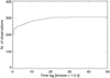 |
Fig. 1 Cumulative histogram of the time lag between consecutive HARPS-N spectra (only data points in the same season are considered). |
2 HARPS-N dataset
We observed, at high cadence, HD 164922 with HARPS-N for five seasons, from March 2013 to October 2017, with an additional set of ten spectra collected between May and June 2018. HARPS-N is a cross-dispersed high-resolution (R = 115 000) echelle spectrograph, in the range 3830–6930 Å. A constant control of its pressure and temperature prevents spectral drifts due to environmental parameters variations. HARPS-N is fed by two fibres: the target feeds the first fibre while the second one can be illuminated either by the sky or a simultaneous calibration source. To obtain high precision in our RV measurements, we exploited the latter technique. We collected a total of 314 spectra with a mean signal-to-noise ratio (S/N) of 200 at 5500 Å and a mean integration time of 600 s. Figure 1 shows the cumulative distribution of the time lag between consecutive data points in our sampling. To account for spectra collected with a time difference slightly larger than one day, as it can happen the night following one observation, we binned the distribution at 1.5 days. Within the same season, ~80% of our spectra were collected with a time lag less or equal to one week, while 65% were taken in contiguous nights or in the same night. The largest difference is 46 days while in the second, third, and fourth seasons we collected two spectra in the same night, with a time lag of about three hours.
The spectra were reduced through the HARPS-N Data Reduction Software (DRS), including the radial velocity extraction based on the Cross-Correlation Function (CCF) method (see Pepe et al. 2002 and the references therein), where the observed spectrum is correlated with a K5 template, called “mask”, depicting the features of a star with spectral type K5V. The offline version of the HARPS-N DRS, which is implemented at the INAF Trieste Observatory1, can be run by the users to re-process the data through the YABI workflow interface (Hunter et al. 2012), with the possibility of modifying the default parameters obtaining thus a custom reduction. The resulting CCF is the weighted and scaled average of the lines contained inthe correlation mask, and can be used as a proxy for common line profile changes. For this reason, it can be analysed through several diagnostics in order to investigate effects related to stellar activity. For instance, Lanza et al. (2018) describe a procedure for deriving a set of CCF asymmetry indicators such as the Bisector Inverse Slope (BIS, e.g. Queloz et al. 2001), the Vasy(mod) (re-adapted from the original definition by Figueira et al. 2013), and the ΔV (Nardetto et al. 2006). With YABI, it is also possible to calculate the chromospheric activity index from the H&K lines of Ca II (S-index and log R’HK) as introduced by Noyes et al. (1984), through a procedure described in Lovis et al. (2011). Finally, we obtained the activity index based on the Hα line following the recipe in Gomes da Silva et al. (2011) and references therein. The HARPS-N RVs,  and BIS time series are listed in Table 1 with the corresponding uncertainties. We excluded from the time series one outlier (BJDTDB = 2 456 410.6424, with an RV deviating of about 20 m s−1 from the expected distribution) and one spectrum due to poor S/N (BJDTDB = 2 457 154.5097, S∕N = 43, RVErr = 1.9 m s−1).
By using the definition in Dravins et al. (1999), we were able to estimate the perspective acceleration of HD 164922, adopting the parallax andthe proper motions listed in Table 2. We therefore noticed that this target shows the non-negligible value of 0.26 m s−1 yr−1, so we decided to apply this correction to our RVs (this is not taken into account by the HARPS-N DRS). The following analysis is therefore performed on the corrected RVs, shown in Fig. 2. The mean uncertainty of the RV measurements is 0.4 m s−1.
Time series of the HARPS-N spectra for HD 164922.
3 Stellar parameters
The main stellar parameters of HD 164922 are collected in Table 2, either reported from the literature or specifically estimated in the present work. The astrometric parameters (positions, proper motions and parallax) are taken from the Gaia Data Release 2 (Gaia Collaboration 2018; Lindegren et al. 2018), that we used to evaluate the perspective acceleration in the previous section.
To estimate the photospheric parameters, we produced a coadded spectrum from 212 HARPS-N spectra of our dataset with higher S/N. We also excluded spectra collected before JD 2 456 740 (March 2014), which are affected by a certain degree of de-focussing (we note that this issue had a negligible impact on the HARPS-N RVs, see Benatti et al. 2017). The S/N of the coadded spectrum reached the high value of 2800. At this level we were mainly limited by systematic errors of the atmospheric parameters determination method rather than by the quality of this spectrum. We obtained a first determination of the atmospheric parameters using CCFPams (Malavolta et al. 2017). By using the most recent release of the MOOG code (Sneden 1973) and following the approach described in Biazzo et al. (2011) with the line list presented in Biazzo et al. (2012), we measured the stellar effective temperature (Teff), surface gravity (log g), iron abundance ([Fe∕H]), and microturbulence velocity vmicro from line equivalent widths (see Table 2). The projected rotational velocity was estimated with the same code and applying the spectral synthesis method after fixing the macroturbulence. Assuming vmacro = 2.6 km s−1 from the relationship by Doyle et al. (2014) based on asteroseismic analysis of main sequence stars observed by the NASA – Kepler satellite and depending on Teff and log g, we find a projected rotational velocity of v sin i = 0.7 ± 0.5 km s−1. This value is consistent with the determination by Brewer et al. (2016), obtained through the spectral synthesis modelling of HIRES datafrom a large sample of dwarfs and subgiants stars. However, since the velocity resolution of HARPS-N is about 2.0 km s−1 we cannot assert that we resolve the actual stellar rotation velocity. We estimated the stellar luminosity by combining parallax measurements with the bolometric corrections to obtain the bolometric magnitude. By using a bolometric correction BC = −0.164 ± 0.11 deduced here by following Buzzoni et al. (2010), we obtained L∕L⊙ = 0.71 ± 0.15. To obtain the mass, radius and age of our target we used the web interface of the Bayesian tool PARAM2 version1.3 (da Silva et al. 2006; Rodrigues et al. 2014), based on the PARSEC isochrones (Bressan et al. 2012). The input parameters are Teff, [Fe∕H], and log g all used as priors to compute the probability density function of the stellar parameters. We found that the resulting fundamental parameters of this star are: age = 9.2 ± 2.5 Gyr, stellar mass M = 0.93 ± 0.05 M⊙ and radius R = 0.95 ± 0.1 R⊙.
The systemic RV and the activity index of the Ca II H&K lines,  , are finally obtained from our HARPS-N dataset. The former is obtained from the orbital fit presented in Sect. 5.2. The evaluation of the
  is not affected by the interstellar reddening being our target within 75 pc (see e.g. Mamajek & Hillenbrand 2008), and its small value, −5.075 ± 0.010, suggests that HD 164922 is a quiet star. According to the empirical relations by Noyes et al. (1984) and Mamajek & Hillenbrand (2008) we should expect a rotation period ranging between 43 and 48 days. In Table 2 we report the adopted Prot,
  days, as derived in Sect. 4.2.
Stellar parameters of HD 164922.
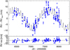 |
Fig. 2 HARPS-N RV time series overimposed on the two planets model (grey line) obtained from the orbital solution presented by F2016 and the corresponding residuals (lower panel). The correction for the perspective acceleration is applied. |
4 HARPS-N time series analysis
In this section, we present a first evaluation of the HARPS-N time series of HD 164922, obtained as described in Sect. 2. This investigation was performed in preparation for the GP analysis presented in Sect. 5.
4.1 Periodogram analysis
We carried out a preliminary two-planets fit of the HARPS-N RVs time series using the MPFIT IDL package3, implemented as in Desidera et al. (2011), starting from the orbital solution reported by F2016 and depicted by a grey solid line in Fig. 2. Subsequently, we computed the Generalised Lomb-Scargle (GLS) periodogram (Zechmeister & Kürster 2009) of the RV residuals, shown in Fig. 3 together with the corresponding window function, in the inset plot. Except for the 1-yr signal located at the lower frequencies, two main periodicities are visible: the dominant one is found at 0.0239 days−1 (i.e. 41.63 d in the time domain, red dashed line), the second one at 0.0803 days−1 (12.46 d, blue dashed line), both of them with a False Alarm Probability (FAP) less than 10−5, evaluated with 10 000 bootstrap random permutations. The large peak at ~ 41.6 d could be the signature of the stellar rotation, as expected by the empirical activity-rotation relationships (Sect. 3), while the second peak could suggest the presence of a short period planetary companion. For sake of completeness, the periodicity at about 0.165 days−1 shows a high value of the FAP (15%). In order to understand whether the main periodicities are related to the stellar activity, we evaluated the GLS for the BIS, the log  and the available asymmetry indices, as presented by Lanza et al. (2018). The GLS of all these parameters are reported in Fig. 4, where the dashed lines follow the same colour code as in Fig. 3. No significant peak can be found close to the 12.46 d periodicity. Based on the FAP evaluation, none of the periodogram peaks appears significant, with the only exception of the 23.4 days in the periodogram of Hα (FAP = 0.01%).
We finally evaluated the Spearman correlation coefficient between the RV residuals of the two-planets fit and the considered activity indices but no correlation was found. This might be explained by the dominant contribution of the faculae to the RVs rather than starspots (e.g. Dumusque 2016 and Collier Cameron et al. 2019 for the solar case).
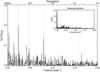 |
Fig. 3 Generalised Lomb-Scargle periodogram of the HARPS-N RV residuals of the two-planets fit. Dashed red and blue lines indicate the periodicities of 41.63 and 12.46 days with the corresponding harmonics (dotted lines). In the inset, the corresponding window function. |
4.2 GP regression of the log R index
index
To confirm the hypothesis that the rotation period of the star is about 42 days, we performed a GP regression analysis of the time series of the log  index. We used a quasi-periodic model for the correlated signal of stellar origin. We first removed all the spectra with S∕N < 20 in theregion of the Ca II lines, to work with a more reliable determination of the log
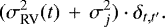
  value. The Monte Carlo analysis has been done with the open source Bayesian inference tool MULTINESTV3.10 (e.g. Feroz et al. 2019), through the PYMULTINEST python wrapper (Buchner et al. 2014), including the publicly available GP python module GEORGEv0.2.1 (Ambikasaran et al. 2015). The formalism used for the GP regression is the same described in Affer et al. (2016), with the quasi-periodic kernel described by the following covariance matrix:
![Mathematical equation: \begin{eqnarray*}k(t, t^{\prime}) &=& h^2\cdot\exp\left[-\frac{(t-t^{\prime})^2}{2\lambda^2} - \frac{\sin^{2}(\pi(t-t^{\prime})/\theta)}{2w^2}\right] \nonumber \\ &&+\, (\sigma^{2}_{\log {R}^{\prime}_{\textrm{HK}}}(t))\cdot\delta_{t, t^{\prime}}, \end{eqnarray*}](/articles/aa/full_html/2020/07/aa37939-20/aa37939-20-eq11.png) (1)
(1)
where t and t′ (t) indicate two different epochs,  is the uncertainty of the log
  index at the time t added quadratically to the diagonal of the covariance matrix, and
  is the Kronecker delta. Finally, h, λ, θ and w are the hyper-parameters: θ represents the periodic time-scale of the modeled signal, and corresponds to the stellar rotation period; h denotes the scale amplitude of the correlated signal; w describes the level of high-frequency variation within a complete stellar rotation; λ represents the decay timescale in days of the correlations and can be physically related to the active region lifetimes (see e.g. Haywood et al. 2014). We performed a run using a uniform prior on θ between 15 and 100 days, large enough to span the range of the possible rotation periods. The resulting posterior distribution for θ shows a maximum centred at
  days, which is close to the expected rotation period as derived from the empirical relation with the value of log
  . Also the maximum a posteriori probability (MAP) value of θ is 42.2 days. The hyper-parameter λ is
  days (MAP = 35.3 days). This value iscomparable to θ, thus it indicates that the correlated signal due to the stellar activity changes within a single rotation period and is well described by a quasi-periodic signal modulated over the stellar rotation period. To complete our analysis on the activity indicators, we run similar models both for the BIS and the Vasy(mod) with large uniform priors on θ (from 0 to 100 days) but no periodicity is found.
In conclusion, our GP analysis of the HARPS-N time series of the log  activity index returned clear evidence for the presence of a 42-d periodicity, that we assume as the rotation period of our target. This period is also very close to the signal of 41.7 days reported by F2016 in the periodogram of their RV data (with an amplitude of 1.9 ms−1) and interpreted as a possible signature of the stellar rotation. However, as their analysis was focussed on the detection of new planetary companions, they did not investigate in detail the nature of that signal.
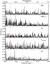 |
Fig. 4 Generalised Lomb-Scargle periodogram of the HARPS-N time series of activity indicators (bisector span,
log |

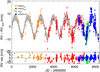 |
Fig. 5 Full RV dataset available in the literature for HD 164922. The grey solid line represents the two-planet model obtained from the solution in F2016 with the corresponding residuals (lower panel). The colour code is defined in the legend. |
4.3 Comparison with data from the literature
As a final check before starting the GP modelling of our RV data, we analysed the rich RV dataset available in the literature for HD 164922. We considered the official HIRES/Keck data release (Butler et al. 2017) and the Levy/APF RVs published by F2016. Both HIRES and Levy spectrographs adopted the Iodine cell method (Butler et al. 1996) to obtain high precision radial velocity measurements. With this technique a rich forest of I2 lines is overimposed on the stellar spectrum as a stable reference in the wavelength range between 5000 and 6200 Å. Similarly to F2016, we considered the HIRES dataset as two separate time series because of the major upgrade of the spectrograph in 2004, labelling them as “pre” and “post” the modification. The HIRESpre dataset includes 51 spectra collected through 8 yr with a mean RV error of 1.23 m s−1. The HIRESpost dataset includes 248 RVs spanning 10 yr with a mean internal error of 1.11 m s−1. Both of them clearly show the modulation of the long period giant planet. The perspective acceleration in the HIRES data is already taken into account by the standard RV extraction pipeline (e.g. Howard et al. 2010). The 73 data from the Levy spectrograph show an RV error of 2.13 m s−1 and do not allow to sample the full orbit of the planet b, since they were specifically collected to recover the planet c (the time span is 1.28 yr).
The full HIRES+Levy+HARPS-N dataset for HD 164922 is probably one of the richest high-precision RV collections known in the literature, since it is composed by 684 data. It is shown in Fig. 5 together with the two-planet fit (grey solid line) obtained as in Sect. 4.1.
The GLS of the corresponding residuals is shown separately for the HIRESpre, HIRESpost and Levy datasets in Fig. 6. As a reference, we overplotted the location of the periodicities found in the HARPS-N residuals with the corresponding harmonics (same colour code as in Fig. 3). We observe a periodicity close to 41.63 d in the HIRESpre dataset, and some power both in the HIRESpost and Levy GLS, even if the peaks are not significantly higher than the background noise. This is expected because of the typical lack of coherence of the stellar rotation modulation. The signal at 12.46 d is not recovered in the HIRESpre data because of the sparse sampling, while it is recognised among the peaks in the HIRESpost GLS. In the Levy GLS the periodicity at 12.46 d is clearly found, while the dominant peak (at about 9.13 days) seems to be spurious after an inspection with 10 000 bootstrap random permutations, similarly for the peak at 5.3 days in the HIRESpre GLS (FAP >5%).
Due to the large time span of the dataset from the literature, that is useful to constrain the orbit of planet b, we included those data in the GP modelling presented in the next section. As a final note, during the preparation of the present work, we learned of an alternative RV extraction of HIRES data from Tal-Or et al. (2019). After the comparison between the two datasets, that showed a typical difference of the RVs of about 0.5 m s−1, we decided to proceed with the data from the official pipeline by Butler et al. (2017).
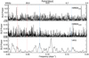 |
Fig. 6 GLS of the RV residuals for the three datasets available in the literature (HIRES “pre” and “post” the major upgrades and Levy). Vertical lines follow the same colour code as in Fig. 3. |
5 Analysis of the radial velocity datasets
For the RV analysis, we used the same tools described in Sect. 4.2, with 800 random walkers and a sampling efficiency of 0.8 The covariance matrix is similar to Eq. (1), but in this case, we added quadratically an uncorrelated noise term defined as:
 (2)
(2)
In this case, σRV(t) is the RV uncertainty at the time t and σj is the additional noise we used to take into account instrumental effects and further noise sources. We performed a GP analysis of the data from HIRES (“pre” and “post”), Levy, and HARPS-N data. The final, multi-instrument dataset is composed by 684 RVs covering a time span of nearly 22 yr, for which a GP regression including two or more Keplerian signals represents a huge computational effort (from a few weeks to months).
5.1 Two-planet model
First of all, we explored the model composed from two Keplerian signals (i.e. planet b and c) including the correlated term due to the stellar activity, modelled by a GP quasi-periodic kernel. The priors for the GP hyper-parameters and for the planetary orbital parameters are reported in Table 3. For λ and w we chose the same conservative priors used to model the log  time series in Sect. 4.2, while we extended the prior on θ in the range 30–50 days. We consider this a choice justified by the large temporal extent of the dataset, since we can expect a change in the measured value of the stellar rotation period over 22 yr, according to the evolution of the activity cycle.
Concerning the two Keplerian signals we chose not to impose Gaussian priors centered on the orbital solution obtained by F2016: this would be too restrictive, given the inclusion of so many new data extending the time span by more than five years. Moreover, since the HIRES data are included in our analysis, it would be improper to adopt an informative prior based on the same data. Finally, we included a linear term as a free parameter of the model to investigate the presence of a long-term additional signal. The results are reported in Table 3. We first notice that the introduction of the HIRES datasets have necessarily impacted on the activity description of the star, with respect to the analysis performed in Sect. 4.2 for HARPS-N data only. On a 22-yr timespan, we could expect rotation period variations due to differential rotation or variation of the magnetic activity cycle, so the hyper-parameter θ changed slightly from the expected 42.3 to 41 days. This can also explain the higher uncertainty on θ, with respect to the GP regression in the case of the HARPS-N time series only, obtained in five years of intensive monitoring.
The GLSof the residuals (Fig. 7) shows the same periodicities identified in Fig. 3, that is the signature of the stellar activity (0.02394 ± 2 × 10⁻⁵ days−1 corresponding to 41.77 ± 0.03 days) and the signal at0.08027 ± 2 × 10⁻⁵ days−1, corresponding to a period of 12.457 ± 0.030 days. If we subtract from these residuals the model of the stellar activity as obtained by the GP regression, the final time series does not show any periodicity, not even the one at ~12.46 days. In this case, the flexibility of the GP regression, likely implied that the activity-induced term has absorbed the candidate third planetary signal. For this reason we modelled the data including one additional Keplerian signal to investigate the nature of the periodicity at ~12.46 days, as described in the next sub-section.
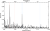 |
Fig. 7 GLS of the RV residuals of the two-planets fit for the full dataset of HD 164922. Same colour code as Fig. 3. |
5.2 Three-planet model
The presence in our data of the robust additional signal at nearly 12.46 days led us to include a third Keplerian signal in the global stellar activity+planet model. We kept fixed the priors for both the activity and the two known planets with respect to the model presented in Sect. 5.1, while the priors for the parameters of the candidate planet d are reported in Table 3. Despite the very precise determination of the signal in the GLS periodogram in Fig. 7, we used a uniform prior for the orbital period in a relatively wide range with the specific aim to avoid biasing the solution toward that value.
Table 3 shows the result of the fit. The description of the correlated activity term is consistent with the one obtained for the two-planet model. The orbital period of the planetary candidate is 12.458 ± 0.003 days, the RV semi-amplitude is 1.3 ± 0.2 m s−1 (6σ significance), and the minimum mass, md sin id = 4 ± 1 M⊕, is 4σ significant.
The best-fit values of the Keplerian parameters are consistent with those by F2016 within 1σ, except for the eccentricity of planet b that we find to be lower and significantly consistent with zero (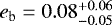 with respect to 0.126 ± 0.049 in F2016). A more constrained eccentricity consistent with zero is also found for planet c (i.e.
  versus 0.22 ± 0.13 from F2016). The model returned a small but significant acceleration term which is found to be correlated to the RV offsets associated to the four instruments. We evaluated the difference of the proper motion components from hipparcos and Gaia DR2 with respect to the reference proper motion from the catalog of accelerations by Brandt (2018). In both cases, the Δμα,δ are lower than 1 mas yr−1 and compatible with zero within 1σ, hinting at a non-existent or negligible anomaly from a purely linear motion on the plane of the sky.
Upper panel of Fig. 8 shows the GLS of the resulting RV residuals after removing the three planetary signals and the instrumental offsets from the original dataset. Except for the periodicity at ~ 42 days and its first harmonics, we notice a peak close to 1-yr signal (0.0028 d−1, which was also present in the two-planet fit residuals in Fig. 7). We performed a pre-whitening operation (where the signal of the most prominent periodicity in the GLS is subtracted from the time series and the main signal in the GLS is evaluated for the residuals and subtracted again until no peaks are above 3σ from the noise) and after the iterative subtraction of the 42 days (GLS in the middle panel of Fig. 8) and the 1-yr signals,the resulting periodogram shows no significant periodicities (lower panel). The origin of the 1-yr periodicity will be discussed in Sect. 6.1. As pointed out in the previous sub-section, the signal of the third planetat about 12.46 days is absorbed in the GP regression, while we demonstrated that it is actually present in our data and must be included in the model. Indeed, the GLS of the RV residuals after the removal of the two known planets and the stellar contribution clearly show the signal of planet d (Fig. 9). The RV phased diagram of the newly detected planet companion is shown in Fig. 10. This plot shows the crucial contribution of HARPS-N (blue diamonds) to recover the small amplitude Kd, which is of the same order of the RV uncertainties of the HIRES datasets. Finally, we show in Fig. 11 a portion of the time series where both HARPS-N (blue dots) and HIRESpost (red dots) data are present. Here the stellar contribution to the RVs is fitted by our GP quasi-periodic model (orange line, while the shaded region indicates the 1σ confidence interval).
To verify that the GP regression does not alter the planetary parameters of the newly detected planet, we set up simple simulations. We assume that our determined planetary parameters of the two known planets are accurate and that the planet we discovered is well retrieved. We considered only the HARPS-N residuals after removing the three Keplerians, with the activity signal left in the data. We then injected the signal of the third planet in the data using our best-fit solution, then creating three mock datasets by randomly shifting each data point within the error bars (including the jitter term we found for HARPS-N, added in quadrature). Each dataset is fitted with a GP regression and one Keplerian to see if the GP interferes with the planet signals (with the priors in common same as those used for theanalysis of the real data). In the three cases, both the orbital period and the RV semi-amplitude are recovered within the errors and in full agreement with the values reported in Table 3. This demonstrates that the signal of planet d is retrieved accurately and precisely, with no interference with the GP.
Priors and percentiles (16th, 50th, and 84th) of the posterior distributions concerning the analysis of the full RV dataset using a GP quasi-periodic kernel.
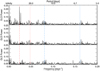 |
Fig. 8 Upper panel: GLS of the RV residuals for the GP regression including three-planets, after removing the instrumental offsets and the planetary signals. Middle and lower panels: GLS of the RV residuals after two iterations of the prewhitening procedure. |
 |
Fig. 9 GLS of the RV residuals after removing planets b and c and the stellar contribution as fitted by the GP model. The signal of planet d at ~ 12.46 days is clearly recovered. |
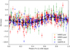 |
Fig. 10 Spectroscopic orbit of planet d. The RV residuals from HIRES (“pre” and “post” upgrade), Levy/APF, and HARPS-N are phase-folded at the orbital period 12.458 days (colour code in the legend, same as in Fig. 5). The residuals are calculated by subtracting the activity-induced term and the signals of planet b and c from the original data, using the results in Table 3. The black solid line represents the best-fit spectroscopic orbit of planet d, while black dots indicate the binned RVs and the error bars represent the RMS of the data in each bin. |
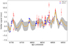 |
Fig. 11 Zoom on the GP quasi-periodic modelling of the stellar signal contribution to the RV times series. The orange line represents the best-fit curve, while the grey shaded area is the confidence interval of 1σ. In this part of the sampling, HARPS-N (blue dots) and HIRESpost (red dots) data overlap. |
5.3 Additional tests
Because the 42-day periodicity persisted through the HIRES/HARPS-N observation time span, we performed a test to confirm that this signature is actually related to stellar activity. Specifically, we analysed the RV residuals of the three-planets fit with the kernel regression (KR) technique, recently applied by Lanza et al. (2018) on a sample of GAPS targets characterised by slow rotation and weak stellar activity. Lanza et al. (2018) show that the KR can model the dependence of the RVs as a function of time and the activity indices (e.g. CCF asymmetry indicators and the log  ), allowing to evaluate the impact of stellar activity on the observed RV time series.
We applied this method to the HARPS-N dataset with the following activity indicators: BIS, ΔV, Vasy(mod), CCF Full Width at Half Maximum (FWHM), CCF contrast and log  . We subdivided the dataset into the six observing seasons, to take into account possible variation of the activity behaviour over the years, which can be better described by different indices. With the KR method, a locally linear model is used to fit the RVs for a well defined time tk. In this way, KR takes into account the temporal variation of the correlation between the RVs and the activity indices, which is expected to be non-linear (Desort et al. 2007). The significance level of the KR modelling for each indicator is estimated through the Fisher-Snedecor statistics, allowing us to identify which indicator better represents the properties of the stellar activity for each observing season. According to Table 4, the best regression is obtained with CCF indicators, while the chromospheric index is preferable only in the fourth and (in the less sampled) sixth season. If we remove the contribution of the activity from the RVs, by using the best model obtained by the KR (see e.g. the modelling relative to the second season in Fig. 12), we observe a remarkable reduction of the RV dispersion (from 2.73 to 0.72 ms−1 for the whole time series, while the decreasing of the dispersion for each season is reported in Table 4) as well as of the power of all the periodicities identified in Fig. 8.
The result of the KR modelling provides an independent confirmation that the RV signal observed at ~42 days is ascribable to the stellar activity and validates the solution of the GP analysis of the log  index presented in Sect. 4.2.
We also employed the Stacked Bayesian General Lomb-Scargle periodogram (SBGLS), proposed by Mortier & Collier Cameron (2017) to discriminate stellar activity from genuine planetary signals of the GLS. Since the activity signals are supposed to be unstable, showing phase incoherence, this method allows to evaluate possible phase-period-amplitude variations of the signal of interest in the classical GLS periodogram calculated as a function of time, that is, with the increasing number of data. Figure 13 shows the SBGLS for the HARPS-N time series of HD 164922 after the removal of the two-planets model, where periodicities are plotted with respect to the increasing number of observations, while the third coordinate represents the Bayesian probability of a specific signal. After gathering ~ 100 data points, boththe signal of planet d and the rotation period become clearly distinguishable and are seen to strengthen with the increasing number of observations. After 150 data, the first harmonics of the rotation period can also be seen. While the 42-day signal is highly significant but not clearly peaked (i.e. the distribution of the power is spread around 42 days, indicated with a blue dashed line together with its first harmonics), the signature of planet d is strictly pointed at 12.46 days, marked with a black dashed line, showing a high Bayesian probability.
Summary of the results of the kernel regression (KR) technique on the HARPS-N RV residuals of the three-planets fit as function of time and of activity indicators.
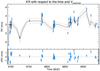 |
Fig. 12 Top panel: HARPS-N RV residuals of the three-planet fit for HD 164922 (second season, same timespan as in Fig. 11) as modelled through the KR with respect to the time and the Vasy(mod). Bottom panel: corresponding residuals. |
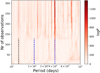 |
Fig. 13 Stacked Bayesian General Lomb-Scargle periodogram applied to the HARPS-N residuals of the two-planets fit. The colour bar indicates the Bayesian probability of the signals. The rotation period with its first harmonics (blue dashed lines) and the orbital period of planet d (black dashed line) are also indicated. |
6 System architecture
In this section, we evaluate the stability of the HD 164922 system and put detection thresholds on additional planets. With this information and the evaluation of the water snow line, we try to infer which formation and migration scenarios could have shaped the current orbital architecture.
6.1 Orbital stability
The long-term stability of the HD 164922 system has been tested as in Benatti et al. (2017), starting from the stellar and planetary parameters in Tables 2 and 3 through the exploration of the phase space around the nominal positions (semi-major axis vs eccentricity) of the three planet companions. We exploited the Frequency Map Analysis (FMA; Laskar 1993; Šidlichovský & Nesvorný 1996; Marzari et al. 2003) tool to evaluate a possible chaotic behaviour of the orbits with short term numerical integrations by analysing the variation of the secular frequencies of the system. We measured the diffusion speed in the phase space, identified by the parameter cV, as the dispersion of the main secular frequency of the system over running windows covering the integration timespan. The results are reportedin Fig. 14 for each planet, starting, left to right, from the super-Earth close to the star, then the Neptune-mass planet and finally the Saturn-mass planet in the outer region. In each of the three models, two of the planets are kept on fixed orbits, the nominal ones, while the orbital parameters of the third planet are randomly changed within a wide interval of values to explore its range of stability in semi-major axis and eccentricity. In each plot, we show the nominal position of the planet and the stability properties of the region around it. The two inner low-mass planets lie within narrow stable zones while the stability region for the outer planet is significantly wider. It means that its orbit can be varied on a broader range without affecting the overall dynamical stability of the system. With the same method, we investigated the possiblestable zones for an additional fourth unseen planet. We set the three known planets on their nominal orbits and randomly select the initial orbital elements of the fourth potential planet adopting for it a mass equal to 1 M⊕. We focussed on the regions between planet d and c (0.1–0.3 au) and between planet c and b (0.4–1.5 au). We did not consider orbits for the fourth planet with semi-major axis smaller than 0.1 au due to the excessive computing load related to the short orbital period.
We found a narrow stable region ranging between 0.18 and 0.21 au, corresponding to an interval of orbital periods from ~30 and ~36 days, therefore, a putative planet with a period of ~42 days should not be permitted, further strengthening our interpretation of the RV signal at this period as the rotation period of the star. A second allowable region is located between 0.6 and 1.4 au (300–500 days), including the habitable zone (HZ) that we evaluated to be 0.95–1.68 aufor the conservative HZ, and 0.75–1.76 au in the optimistic case. The calculation was performed by using the public tool4 based on Kopparapu et al. (2013, 2014), assuming a planet of 1 M⊕ and adopting Teff and stellar luminosity from Table 2.
As mentioned in Sect. 5.2, the GLS of the HARPS-N RVs reveals the presence of a periodicity of ~ 357 days, that we analysed on the light of this latter result. Rather than being due to a planet, this signal has more probably the same origin of thespurious 1-yr signal first reported and characterised by Dumusque et al. (2015) by using HARPS data. For HARPS-N data this feature is also suspected in the GLS periodograms presented in Barbato et al. (2020). As in Fig. 3 from Dumusque et al. (2015), we verified that the RV signal is in opposition of phase with the Earth orbital motion around the Sun, showing a correlation with the Barycentric Earth Radial Velocity (BERV). In the case of HARPS, CCD imperfections lead to a deformation of specific spectral lines passing by the crossing block stitching of the detector. The long observation baseline of HD 164922 with HARPS-N allows to detect this spurious signal since we sample a large variation of the BERV (± 20 km s−1). However, the treatment or the removal of this signal is beyond the scope of the present paper.
6.2 Detectability limits
We computed the detection threshold for the HARPS-N dataset following the Bayesian approach from Tuomi et al. (2014). We applied this technique on the RV residuals after subtracting the signals of the three planets and including in the model the GP to take into account the stellar activity contribution. The resulting detectability map is shown in Fig. 15. Planets b, c and d (red circles) are located above the detection threshold, as expected. HD 164922 d is just above the minimum mass detection threshold, which corresponds to mp sin i = 2.3 M⊕ in the interval 12 < Porb < 13 days. We can also compute the minimum mass threshold in the orbitally-stable regions identified in Sect. 6.1: we obtain a minimum mass limit of 5.0 M⊕ for the 30–36 days region, 18 M⊕ for the 300–500 days region, and a few tens of M⊕ for the P > 1200 d region. In the figure, we indicated with green areas the allowed regions for additional companions in the system, as defined in Sect. 6.1, while the inner part of the system that we did not explored is represented in grey.
6.3 Snow line position of the HD 164922 system
In order to investigate the planetary migration scenario of the HD 164922 system, we estimated the position of the water snow line, that is,the distance from the central star where the midplane temperature of the proto-planetary disk drops down to thesublimation temperature of the water ice (Hayashi 1981), at the classical value of 170 K. Out of the snow line, the surface density of the disk increases by a factor of about three due to the presence of water ice, leading to an increase of the isolation mass (i.e. the mass a body can accrete solely through planetesimal accretion; Lissauer 1987; Lissauer & Stevenson 2007) and of the size of protoplanetary cores. For this reason, the region around the snow line provides a favourable location for forming planets (Stevenson & Lunine 1988; Morbidelli et al. 2015). In order to evaluate the snow line position for the HD 164922 system, we considered a simple Minimum Mass Solar Nebula (MMSN) disk model as in Kennedy & Kenyon (2008), where the surface density of the disk, Σ, changes with time and the distance from the central star (a) as:
 (3)
(3)
where Σ0 = 100 kg m−2, fice represents the increasing of Σ due to ice condensation outside the snow line, and M⋆ is the stellar mass. The factor η provides a range of disk masses for a fixed stellar mass (“relative disk mass”, Kennedy & Kenyon 2008) and is varied to account for the observed range of disk masses at fixed stellar mass. Observations (e.g. Natta et al. 2000) stated that this parameter ranges from 0.5 up to 5 for disk masses between 0.01 and 0.1 M⋆. In the case of HD 164922, we considered η = 4. The midplane temperature of accreting protoplanetary disk irradiated by the central star is given by:
 (4)
(4)
where Tmid,acc is the temperature profile of the midplane due to the mass accretion and the corresponding viscous heating of the disk, and Tirr is the temperature profile of the disk due to the irradiation heating (Sasselov & Lecar 2000; Lecar et al. 2006; Kennedy & Kenyon 2008). For Tirr we considered the scale law obtained by Sasselov & Lecar (2000)5, while for the contribution due to the accretion we considered the standard relation reported in Eq. (1) in Bell et al. (1997) and the dust opacity according to Hubeny (1990)6. For simplicity, we assumed that the dust opacities are constant throughout the disk. To evaluate Tmid,acc, we obtainedthe stellar parameters of HD 164922 in the pre-main sequence (PMS) phase at about 1 Myr of age, exploiting the PARSEC evolutionary tracks. We adopted the set of models with a metallicity of [Fe/H] = 0.18 (from Table 2), corresponding to X = 0.73, Y = 0.25 and Z = 0.02 (Asplund et al. 2004). From this set of models we selected the parameters for masses of 0.90, 0.95 and 1.00 M⊙ at the age of 1 Myr. Stellar parameters were obtained interpolating the values for masses, temperatures, and radii of the three chosen models and they resulted to be R1Myr = 2.31 R⊙, Teff, 1Myr = 4443.3 K. For the accretion rate, we considered the typical value for the MMSN of 10−8 M⊙ yr−1.
Both the passive and the accreting disk temperature profiles are shown in Fig. 16, together with the location of the snow line and the position of the three planets of the HD 164922 system. The snow line position is found to be at 1.03 au for the passive disk and at 1.38 au for the accreting and irradiated disk, thus located about halfway between planet c and b.
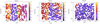 |
Fig. 14 Stability of the three planetary companions of the HD 164922 system as a function of the initial eccentricity and semi-major axis. Colour scale indicates the value of the orbital diffusion speed (cV) ranging from black, representing stable regions, to yellow, which indicates a higher degree of instability for planets with given separation and eccentricity. Nominal positions of the planets are identified with a green circle. From left to right, the planets are represented as a function of the distance from the host star. |
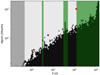 |
Fig. 15 Detection map for the HARPS-N RV residuals of the three-planet fit for the HD 164922 system. The white part corresponds to the area in the period - minimum mass space where additional signals could be detected if present in the data, while the black region corresponds to the area where the detection probability is negligible. The red circles mark the position in the parameter space of the three planets orbiting HD 164922. The green areas denote the stability regions for additional companions (as determined in Sect. 6.1), while the gray area indicates the part of the system not explored by our orbital simulations. |
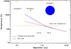 |
Fig. 16 Temperature profile for the midplane of a static disk (solid red line) and an accreting and irradiated protoplanetary disk (solid blue line). The horizontal dashed line shows the position of the snow line considering a value of 170 K for the sublimation temperature of water ice. The edges of the corresponding snow lines are indicated with dotted vertical lines and their distances. The separation of the planets in the system is also shown as a reference. The size of the symbols is proportionalto the planetary masses. |
6.4 Discussion
According to our GP regression, the eccentricities of the three planetary companions of HD 164922 are all consistent with zero (Table 3) and the RV analysis over a time span of 22 yr excludes the presence of outer companions with a mass larger than ~ 30 M⊕ up to 5 au (with a period of about 4000 days, cf Fig. 15), a result corroborated by the negligible value of the Δμα,δ. The lack of a massive perturbing body and the low planetary eccentricities indicate that a migration through the protoplanetary disk could have acted in shaping the present system architecture. Planet b probably formed beyond the water snow line. Due to its relatively low mass it is supposed to have quickly migrated closer to the star until the disk dissipation. The formation of the two low-mass planets, instead, occurred within the snow line. For them, we can consider two possiblescenarios: the in-situ formation, that requires a large amount of solids in the protoplanetary disk within 1 au (Hansen & Murray 2012), and the inside-out model (Chatterjee & Tan 2014), that invokes pebbles formation and their consequent drifting toward the inner region of the disk, stimulating then the planet formation process.
According to Eq. (3) in Hansen & Murray (2012), the minimum mass of HD 164922 d allows in principle to accrete gas from the disk, but its orbital distance also enables the photoevaporation of the same gas (cf Fig. 15 in Hansen & Murray 2012). No high-volatileatmosphere is then expected for this planet. By applying the tidal model of Leconte et al. (2010) with a tidal time lag  , where
  is the modified tidal qualityfactor, a parameterization of the tidal response of the planet’s interior, we find a heat flux across the surface of planet d of 0.8 W m−2 for a radius of 1.3 R⊙ and of 5 W m−2 for a radius of 2.4 R⊙. However, the value of
  appropriate for a planet with a radius of 2.4 R⊙ could be much larger leading to a proportional reduction of the heat flux. For example, adopting
  , that is estimated to be appropriate for Uranus (Ogilvie 2014), we obtain a flux of only 0.05 W m−2. In the case of a rocky planet with
  similar to that of the Earth, planet d may host a significant volcanic activity powered by tidal dissipation in its interior. For comparison, in the case of the volcanic Jupiter moon Io, the heat flux is 2.0−2.6 W m−2 (see Rathbun et al. 2004). The timescale for the tidal decay of the eccentricity of the orbit of planet d is longer than ≈ 6 Gyr even for
  and Rd = 2.4 R⊙, indicating that its possible eccentricity could be primordial, that is, not necessarily excited by the other planets in the system. The original eccentricity of planet d could have been higher, although not high enough to cross the other orbits or destabilize the system. However, the unknown radius and internal structure of planet d prevent us from drawing sound conclusions on its evolution.
Our interpretation and comprehension of the planetary system architecture, formation and evolution rely on the accuracy of the inferred stellar parameters. Unfortunately, the fundamental parameters can be better constrained only by an appropriate asteroseismic campaign. At present we can only predict that the oscillation spectrum of this star should be characterised by approximately a large frequency separation of Δν = 140.6, ∕μHz and a frequency of maximum power of νmax ≃ 3306, ∕μHz obtained by the scaling relation calibrated on solar values given by Kjeldsen & Bedding (1995). The values are interesting when compared to the values of the Sun Δν = 135, ∕μHz and a frequency of maximum power of νmax = 3050, ∕μHz. The hope for the next future is to have the possibility to compare our findings with the asteroseismic data collected for this star.
7 Conclusions
One of the largest high-precision RV datasets available in the literature allowed us to claim the presence of an additional close-in super-Earth with minimum mass md sin id = 4 ± 1 M⊕ in the HD 164922 planetary system, known to host a sub-Neptune-mass planet and a distant Saturn-mass planet. We monitored this target in the framework of the GAPS programme focussed on finding close-in low-mass companions in systems with outer giant planets. Thanks to the dedicated monitoring and the high precision RV measurements ensured by HARPS-N, we took full advantage of the GP regression analysis. With such a technique, we could robustly model the stellar activity as a quasi-periodic signal both from the log  index and the RV time series. The subtraction of this contribution to the RVs allowed us to recover the low-amplitude Keplerian signal of the additional companion at a 6σ level (Kd = 1.3 ± 0.2 m s−1). The application of the Kernel Regression technique to the residuals of the three-planets fit confirmed that the signal content can be properly described as a function of time and the activity indices.
The analysis of the system architecture allowed us to infer that the most probable planet migration process is through the gas of the protoplanetary disk. The challenging detection of HD 164922 d is an example of the observational effort invoked by Zhu & Wu (2018) to find low-mass planets in systems with cold gaseous planets with state-of-the-art instrumentation, because of the very high probability that those systems could host low-mass planets in their interiors. Unfortunately, this target will not be observed with the NASA Transiting Exoplanets Survey Satellite (TESS, Ricker et al. 2015) satellite, at least not in Cycle 2, to verify if it transits. Dedicated observations with the ESA CHarachterizing ExOPlanet Satellite (CHEOPS, Broeg et al. 2013) could be proposed, but they can be severely affected by the uncertainty on the transit time. For instance, at the beginning of 2021 it could be of the order of 0.9 days by using our ephemeris in Table 3. A former attempt to search for transits of planets b and c was reported in F2016 with APT photometry (about 1000data spread over 10 yr), with no evidence of such events or photometric variability between 1 and 100 days. However, their data cadence does not appear to be well-suited for the detection of a potential transit of planet d.
Acknowledgements
The authors acknowledge the anonymous Referee for her/his useful comments and suggestions. The authorsacknowledge the support from INAF through the “WOW Premiale” funding scheme of the Italian Ministry of Education, University, and Research. MD acknowledges financial support from Progetto Premiale 2015 FRONTIERA (OB.FU. 1.05.06.11) funding scheme of the Italian Ministry of Education, University, and Research. We acknowledge financial support from the ASI-INAF agreement n.2018-16-HH.0. We acknowledge the computing centres of INAF – Osservatorio Astronomico di Trieste/Osservatorio Astrofisico di Catania, under the coordination of the CHIPP project, for the availability of computing resources and support. MB acknowledges support from the STFC research grant ST/000631/1. This work has made use of data from the European Space Agency (ESA) mission Gaia (https://www.cosmos.esa.int/gaia), processed by the Gaia Data Processing and Analysis Consortium (DPAC, https://www.cosmos.esa.int/web/gaia/dpac/consortium). Funding for the DPAC has been provided by national institutions, in particular the institutions participating in the Gaia Multilateral Agreement.
References
- Affer, L., Micela, G., Damasso, M., et al. 2016, A&A, 593, A117 [NASA ADS] [CrossRef] [EDP Sciences] [Google Scholar]
- Agnew, M. T., Maddison, S. T., Thilliez, E., & Horner, J. 2017, MNRAS, 471, 4494 [NASA ADS] [CrossRef] [Google Scholar]
- Agnew, M. T., Maddison, S. T., & Horner, J. 2018, MNRAS, 481, 4680 [CrossRef] [Google Scholar]
- Ambikasaran, S., Foreman-Mackey, D., Greengard, L., Hogg, D. W., & O’Neil, M. 2015, IEEE Transac. Pattern Anal. Machine Intell., 38, 2 [Google Scholar]
- Armitage, P. J. 2003, ApJ, 582, L47 [NASA ADS] [CrossRef] [MathSciNet] [Google Scholar]
- Asplund, M., Grevesse, N., Sauval, A. J., Allende Prieto, C., & Kiselman, D. 2004, A&A, 417, 751 [NASA ADS] [CrossRef] [EDP Sciences] [Google Scholar]
- Bailer-Jones, C. A. L., Rybizki, J., Fouesneau, M., Mantelet, G., & Andrae, R. 2018, AJ, 156, 58 [NASA ADS] [CrossRef] [Google Scholar]
- Barbato, D., Sozzetti, A., Desidera, S., et al. 2018, A&A, 615, A175 [NASA ADS] [CrossRef] [EDP Sciences] [Google Scholar]
- Barbato, D., Pinamonti, M., Sozzetti, A., et al. 2020, A&A, submitted [Google Scholar]
- Batalha, N. M., Rowe, J. F., Bryson, S. T., et al. 2013, ApJS, 204, 24 [NASA ADS] [CrossRef] [Google Scholar]
- Bell, K. R., Cassen, P. M., Klahr, H. H., & Henning, T. 1997, ApJ, 486, 372 [NASA ADS] [CrossRef] [Google Scholar]
- Benatti, S., Claudi, R., Desidera, S., et al. 2016, in Frontier Research in Astrophysics II (USA: Proceedings of Science), 69 [Google Scholar]
- Benatti, S., Desidera, S., Damasso, M., et al. 2017, A&A, 599, A90 [NASA ADS] [CrossRef] [EDP Sciences] [Google Scholar]
- Biazzo, K., Randich, S., & Palla, F. 2011, A&A, 525, A35 [NASA ADS] [CrossRef] [EDP Sciences] [Google Scholar]
- Biazzo, K., D’Orazi, V., Desidera, S., et al. 2012, MNRAS, 427, 2905 [NASA ADS] [CrossRef] [Google Scholar]
- Brandt, T. D. 2018, ApJS, 239, 31 [NASA ADS] [CrossRef] [Google Scholar]
- Bressan, A., Marigo, P., Girardi, L., et al. 2012, MNRAS, 427, 127 [NASA ADS] [CrossRef] [Google Scholar]
- Brewer, J. M., Fischer, D. A., Valenti, J. A., & Piskunov, N. 2016, ApJS, 225, 32 [NASA ADS] [CrossRef] [Google Scholar]
- Broeg, C., Fortier, A., Ehrenreich, D., et al. 2013, EPJ Web Conf., 47, 03005 [CrossRef] [EDP Sciences] [Google Scholar]
- Bryan, M. L., Knutson, H. A., Lee, E. J., et al. 2019, AJ, 157, 52 [NASA ADS] [CrossRef] [Google Scholar]
- Buchner, J., Georgakakis, A., Nandra, K., et al. 2014, A&A, 564, A125 [NASA ADS] [CrossRef] [EDP Sciences] [Google Scholar]
- Butler, R. P., Marcy, G. W., Williams, E., et al. 1996, PASP, 108, 500 [NASA ADS] [CrossRef] [Google Scholar]
- Butler, R. P., Wright, J. T., Marcy, G. W., et al. 2006, ApJ, 646, 505 [NASA ADS] [CrossRef] [Google Scholar]
- Butler, R. P., Vogt, S. S., Laughlin, G., et al. 2017, AJ, 153, 208 [NASA ADS] [CrossRef] [Google Scholar]
- Buzzoni, A., Patelli, L., Bellazzini, M., Pecci, F. F., & Oliva, E. 2010, MNRAS, 403, 1592 [NASA ADS] [CrossRef] [Google Scholar]
- Chatterjee, S.,& Tan, J. C. 2014, ApJ, 780, 53 [NASA ADS] [CrossRef] [Google Scholar]
- Collier Cameron, A., Mortier, A., Phillips, D., et al. 2019, MNRAS, 487, 1082 [CrossRef] [Google Scholar]
- Cosentino, R., Lovis, C., Pepe, F., et al. 2014, Proc. SPIE, 9147, 91478C [Google Scholar]
- Covino, E., Esposito, M., Barbieri, M., et al. 2013, A&A, 554, A28 [NASA ADS] [CrossRef] [EDP Sciences] [Google Scholar]
- da Silva, L., Girardi, L., Pasquini, L., et al. 2006, A&A, 458, 609 [NASA ADS] [CrossRef] [EDP Sciences] [Google Scholar]
- Desidera, S., Carolo, E., Gratton, R., et al. 2011, A&A, 533, A90 [NASA ADS] [CrossRef] [EDP Sciences] [Google Scholar]
- Desort, M., Lagrange, A.-M., Galland, F., Udry, S., & Mayor, M. 2007, A&A, 473, 983 [NASA ADS] [CrossRef] [EDP Sciences] [Google Scholar]
- Doyle, A. P., Davies, G. R., Smalley, B., Chaplin, W. J., & Elsworth, Y. 2014, MNRAS, 444, 3592 [NASA ADS] [CrossRef] [Google Scholar]
- Dravins, D., Lindegren, L., & Madsen, S. 1999, A&A, 348, 1040 [NASA ADS] [Google Scholar]
- Dumusque, X. 2016, A&A, 593, A5 [NASA ADS] [CrossRef] [EDP Sciences] [Google Scholar]
- Dumusque, X., Santos, N. C., Udry, S., Lovis, C., & Bonfils, X. 2011a, A&A, 527, A82 [NASA ADS] [CrossRef] [EDP Sciences] [Google Scholar]
- Dumusque, X., Udry, S., Lovis, C., Santos, N. C., & Monteiro, M. J. P. F. G. 2011b, A&A, 525, A140 [NASA ADS] [CrossRef] [EDP Sciences] [Google Scholar]
- Dumusque, X., Pepe, F., Lovis, C., & Latham, D. W. 2015, ApJ, 808, 171 [NASA ADS] [CrossRef] [Google Scholar]
- Egeland, R., Soon, W., Baliunas, S., et al. 2017, ApJ, 835, 25 [NASA ADS] [CrossRef] [Google Scholar]
- Feroz, F., Hobson, M. P., Cameron, E., & Pettitt, A. N. 2019, Open J. Astrophys., 2, 10 [CrossRef] [Google Scholar]
- Figueira, P., Santos, N. C., Pepe, F., Lovis, C., & Nardetto, N. 2013, A&A, 557, A93 [NASA ADS] [CrossRef] [EDP Sciences] [Google Scholar]
- Fulton, B. J., Howard, A. W., Weiss, L. M., et al. 2016, ApJ, 830, 46 [NASA ADS] [Google Scholar]
- Gaia Collaboration (Brown, A. G. A., et al.) 2018, A&A, 616, A1 [NASA ADS] [CrossRef] [EDP Sciences] [Google Scholar]
- Gomes da Silva, J., Santos, N. C., Bonfils, X., et al. 2011, A&A, 534, A30 [NASA ADS] [CrossRef] [EDP Sciences] [Google Scholar]
- Hansen, B. M.S., & Murray, N. 2012, ApJ, 751, 158 [Google Scholar]
- Hatzes, A. P., Cochran, W. D., McArthur, B., et al. 2000, ApJ, 544, L145 [NASA ADS] [CrossRef] [Google Scholar]
- Hayashi, C. 1981, Prog. Theor. Phys. Suppl., 70, 35 [NASA ADS] [CrossRef] [MathSciNet] [Google Scholar]
- Haywood, R. D., Collier Cameron, A., Queloz, D., et al. 2014, MNRAS, 443, 2517 [NASA ADS] [CrossRef] [Google Scholar]
- Howard, A. W., Johnson, J. A., Marcy, G. W., et al. 2010, ApJ, 721, 1467 [NASA ADS] [CrossRef] [Google Scholar]
- Hubeny, I. 1990, ApJ, 351, 632 [NASA ADS] [CrossRef] [Google Scholar]
- Hunter, A., Macgregor, A., Szabo, T., Wellington, C., & Bellgard, M. 2012, Source Code Biol. Med., 7, 1 [CrossRef] [Google Scholar]
- Izidoro, A., Raymond, S. N., Morbidelli, A. r., Hersant, F., & Pierens, A. 2015, ApJ, 800, L22 [NASA ADS] [CrossRef] [Google Scholar]
- Kennedy, G. M., & Kenyon, S. J. 2008, ApJ, 673, 502 [NASA ADS] [CrossRef] [Google Scholar]
- Kjeldsen, H., & Bedding, T. R. 1995, A&A, 293, 87 [NASA ADS] [Google Scholar]
- Kopparapu, R. K., Ramirez, R., Kasting, J. F., et al. 2013, ApJ, 765, 131 [NASA ADS] [CrossRef] [Google Scholar]
- Kopparapu, R. K., Ramirez, R. M., SchottelKotte, J., et al. 2014, ApJ, 787, L29 [NASA ADS] [CrossRef] [Google Scholar]
- Lanza, A. F., Malavolta, L., Benatti, S., et al. 2018, A&A, 616, A155 [NASA ADS] [CrossRef] [EDP Sciences] [Google Scholar]
- Laskar, J. 1993, Physica D Nonlinear Phenomena, 67, 257 [Google Scholar]
- Lecar, M., Podolak, M., Sasselov, D., & Chiang, E. 2006, ApJ, 640, 1115 [Google Scholar]
- Leconte, J., Chabrier, G., Baraffe, I., & Levrard, B. 2010, A&A, 516, A64 [NASA ADS] [CrossRef] [EDP Sciences] [Google Scholar]
- Lindegren, L., Hernández, J., Bombrun, A., et al. 2018, A&A, 616, A2 [NASA ADS] [CrossRef] [EDP Sciences] [Google Scholar]
- Lissauer, J. J. 1987, Icarus, 69, 249 [NASA ADS] [CrossRef] [Google Scholar]
- Lissauer, J. J., & Stevenson, D. J. 2007, Protostars and Planets V (Tucson: University of Arizona Press), 591 [Google Scholar]
- Lovis, C., Dumusque, X., Santos, N. C., et al. 2011, ArXiv eprints [arXiv:1107.5325] [Google Scholar]
- Malavolta, L., Lovis, C., Pepe, F., Sneden, C., & Udry, S. 2017, MNRAS, 469, 3965 [NASA ADS] [CrossRef] [Google Scholar]
- Mamajek, E. E., & Hillenbrand, L. A. 2008, ApJ, 687, 1264 [NASA ADS] [CrossRef] [Google Scholar]
- Mandell, A. M., Raymond, S. N., & Sigurdsson, S. 2007, ApJ, 660, 823 [NASA ADS] [CrossRef] [Google Scholar]
- Markwardt, C. B. 2009, ASP Conf. Ser., 411, 251 [Google Scholar]
- Marzari, F., Tricarico, P., & Scholl, H. 2003, MNRAS, 345, 1091 [NASA ADS] [CrossRef] [Google Scholar]
- Matsumura, S., Ida, S., & Nagasawa, M. 2013, ApJ, 767, 129 [NASA ADS] [CrossRef] [Google Scholar]
- Mayor, M., Udry, S., Naef, D., et al. 2004, A&A, 415, 391 [NASA ADS] [CrossRef] [EDP Sciences] [Google Scholar]
- Morbidelli, A., Lambrechts, M., Jacobson, S., & Bitsch, B. 2015, Icarus, 258, 418 [NASA ADS] [CrossRef] [Google Scholar]
- Mortier, A., & Collier Cameron, A. 2017, A&A, 601, A110 [NASA ADS] [CrossRef] [EDP Sciences] [Google Scholar]
- Nardetto, N., Mourard, D., Kervella, P., et al. 2006, A&A, 453, 309 [NASA ADS] [CrossRef] [EDP Sciences] [Google Scholar]
- Natta, A., Grinin, V., & Mannings, V. 2000, Protostars and Planets IV (Tucson: University of Arizona Press), 559 [Google Scholar]
- Noyes, R. W., Hartmann, L. W., Baliunas, S. L., Duncan, D. K., & Vaughan, A. H. 1984, ApJ, 279, 763 [NASA ADS] [CrossRef] [Google Scholar]
- Ogilvie, G. I. 2014, ARA&A, 52, 171 [Google Scholar]
- Pepe, F., Mayor, M., Galland, F., et al. 2002, A&A, 388, 632 [NASA ADS] [CrossRef] [EDP Sciences] [Google Scholar]
- Queloz, D., Henry, G. W., Sivan, J. P., et al. 2001, A&A, 379, 279 [NASA ADS] [CrossRef] [EDP Sciences] [Google Scholar]
- Rathbun, J. A., Spencer, J. R., Tamppari, L. K., et al. 2004, Icarus, 169, 127 [NASA ADS] [CrossRef] [Google Scholar]
- Ricker, G. R., Winn, J. N., Vanderspek, R., et al. 2015, J. Astron. Teles. Instrum. Sys. 1, 014003 [Google Scholar]
- Rodrigues, T. S., Girardi, L., Miglio, A., et al. 2014, MNRAS, 445, 2758 [NASA ADS] [CrossRef] [Google Scholar]
- Sánchez, M. B., de Elía, G. C., & Darriba, L. A. 2018, MNRAS, 481, 1281 [NASA ADS] [CrossRef] [Google Scholar]
- Sasselov, D. D., & Lecar, M. 2000, ApJ, 528, 995 [NASA ADS] [CrossRef] [Google Scholar]
- Šidlichovský, M., & Nesvorný, D. 1996, Celest. Mech. Dyn. Astron., 65, 137 [NASA ADS] [CrossRef] [Google Scholar]
- Sneden, C. 1973, ApJ, 184, 839 [NASA ADS] [CrossRef] [Google Scholar]
- Stevenson, D. J., & Lunine, J. I. 1988, Icarus, 75, 146 [NASA ADS] [CrossRef] [Google Scholar]
- Tal-Or, L., Trifonov, T., Zucker, S., Mazeh, T., & Zechmeister, M. 2019, MNRAS, 484, L8 [NASA ADS] [CrossRef] [Google Scholar]
- Thébault, P., Marzari, F., & Scholl, H. 2002, A&A, 384, 594 [NASA ADS] [CrossRef] [EDP Sciences] [Google Scholar]
- Tuomi, M., Jones, H. R. A., Barnes, J. R., Anglada-Escudé, G., & Jenkins, J. S. 2014, MNRAS, 441, 1545 [NASA ADS] [CrossRef] [Google Scholar]
- van Leeuwen, F. 2007, A&A, 474, 653 [NASA ADS] [CrossRef] [EDP Sciences] [Google Scholar]
- Weiss, L. M., Marcy, G. W., Petigura, E. A., et al. 2018, AJ, 155, 48 [NASA ADS] [CrossRef] [Google Scholar]
- Zechmeister, M., & Kürster, M. 2009, A&A, 496, 577 [NASA ADS] [CrossRef] [EDP Sciences] [Google Scholar]
- Zhu, W., & Wu, Y. 2018, AJ, 156, 92 [NASA ADS] [CrossRef] [Google Scholar]
A non-linear least squares curve fitting presented by Markwardt (2009), available at http://purl.com/net/mpfit
Tirr(a) = T0a−3∕7, with  (e.g. for M⋆ = 0.5
M⊙,
T0 is equal to 140 K), where the opacity k
is 0 ≤ k < 2.
(e.g. for M⋆ = 0.5
M⊙,
T0 is equal to 140 K), where the opacity k
is 0 ≤ k < 2.
 , where
Teff,acc is the effective temperature of a given ring of a disk, defined as
, where
Teff,acc is the effective temperature of a given ring of a disk, defined as  , where Ṁ is the accretion rate, R⋆ is the stellar radius, and σ
is the Stefan’s constant.
, where Ṁ is the accretion rate, R⋆ is the stellar radius, and σ
is the Stefan’s constant.
All Tables
Priors and percentiles (16th, 50th, and 84th) of the posterior distributions concerning the analysis of the full RV dataset using a GP quasi-periodic kernel.
Summary of the results of the kernel regression (KR) technique on the HARPS-N RV residuals of the three-planets fit as function of time and of activity indicators.
All Figures
|
Fig. 1 Cumulative histogram of the time lag between consecutive HARPS-N spectra (only data points in the same season are considered). |
| In the text | |
|
Fig. 2 HARPS-N RV time series overimposed on the two planets model (grey line) obtained from the orbital solution presented by F2016 and the corresponding residuals (lower panel). The correction for the perspective acceleration is applied. |
| In the text | |
|
Fig. 3 Generalised Lomb-Scargle periodogram of the HARPS-N RV residuals of the two-planets fit. Dashed red and blue lines indicate the periodicities of 41.63 and 12.46 days with the corresponding harmonics (dotted lines). In the inset, the corresponding window function. |
| In the text | |
|
Fig. 4 Generalised Lomb-Scargle periodogram of the HARPS-N time series of activity indicators (bisector span,
log |
| In the text | |
|
Fig. 5 Full RV dataset available in the literature for HD 164922. The grey solid line represents the two-planet model obtained from the solution in F2016 with the corresponding residuals (lower panel). The colour code is defined in the legend. |
| In the text | |
|
Fig. 6 GLS of the RV residuals for the three datasets available in the literature (HIRES “pre” and “post” the major upgrades and Levy). Vertical lines follow the same colour code as in Fig. 3. |
| In the text | |
|
Fig. 7 GLS of the RV residuals of the two-planets fit for the full dataset of HD 164922. Same colour code as Fig. 3. |
| In the text | |
|
Fig. 8 Upper panel: GLS of the RV residuals for the GP regression including three-planets, after removing the instrumental offsets and the planetary signals. Middle and lower panels: GLS of the RV residuals after two iterations of the prewhitening procedure. |
| In the text | |
|
Fig. 9 GLS of the RV residuals after removing planets b and c and the stellar contribution as fitted by the GP model. The signal of planet d at ~ 12.46 days is clearly recovered. |
| In the text | |
|
Fig. 10 Spectroscopic orbit of planet d. The RV residuals from HIRES (“pre” and “post” upgrade), Levy/APF, and HARPS-N are phase-folded at the orbital period 12.458 days (colour code in the legend, same as in Fig. 5). The residuals are calculated by subtracting the activity-induced term and the signals of planet b and c from the original data, using the results in Table 3. The black solid line represents the best-fit spectroscopic orbit of planet d, while black dots indicate the binned RVs and the error bars represent the RMS of the data in each bin. |
| In the text | |
|
Fig. 11 Zoom on the GP quasi-periodic modelling of the stellar signal contribution to the RV times series. The orange line represents the best-fit curve, while the grey shaded area is the confidence interval of 1σ. In this part of the sampling, HARPS-N (blue dots) and HIRESpost (red dots) data overlap. |
| In the text | |
|
Fig. 12 Top panel: HARPS-N RV residuals of the three-planet fit for HD 164922 (second season, same timespan as in Fig. 11) as modelled through the KR with respect to the time and the Vasy(mod). Bottom panel: corresponding residuals. |
| In the text | |
|
Fig. 13 Stacked Bayesian General Lomb-Scargle periodogram applied to the HARPS-N residuals of the two-planets fit. The colour bar indicates the Bayesian probability of the signals. The rotation period with its first harmonics (blue dashed lines) and the orbital period of planet d (black dashed line) are also indicated. |
| In the text | |
|
Fig. 14 Stability of the three planetary companions of the HD 164922 system as a function of the initial eccentricity and semi-major axis. Colour scale indicates the value of the orbital diffusion speed (cV) ranging from black, representing stable regions, to yellow, which indicates a higher degree of instability for planets with given separation and eccentricity. Nominal positions of the planets are identified with a green circle. From left to right, the planets are represented as a function of the distance from the host star. |
| In the text | |
|
Fig. 15 Detection map for the HARPS-N RV residuals of the three-planet fit for the HD 164922 system. The white part corresponds to the area in the period - minimum mass space where additional signals could be detected if present in the data, while the black region corresponds to the area where the detection probability is negligible. The red circles mark the position in the parameter space of the three planets orbiting HD 164922. The green areas denote the stability regions for additional companions (as determined in Sect. 6.1), while the gray area indicates the part of the system not explored by our orbital simulations. |
| In the text | |
|
Fig. 16 Temperature profile for the midplane of a static disk (solid red line) and an accreting and irradiated protoplanetary disk (solid blue line). The horizontal dashed line shows the position of the snow line considering a value of 170 K for the sublimation temperature of water ice. The edges of the corresponding snow lines are indicated with dotted vertical lines and their distances. The separation of the planets in the system is also shown as a reference. The size of the symbols is proportionalto the planetary masses. |
| In the text | |
Current usage metrics show cumulative count of Article Views (full-text article views including HTML views, PDF and ePub downloads, according to the available data) and Abstracts Views on Vision4Press platform.
Data correspond to usage on the plateform after 2015. The current usage metrics is available 48-96 hours after online publication and is updated daily on week days.
Initial download of the metrics may take a while.