| Issue |
A&A
Volume 639, July 2020
|
|
|---|---|---|
| Article Number | A9 | |
| Number of page(s) | 13 | |
| Section | Planets and planetary systems | |
| DOI | https://doi.org/10.1051/0004-6361/202037458 | |
| Published online | 01 July 2020 | |
New multi-part collisional model of the main belt: the contribution to near-Earth asteroids
1
Instituto de Astrofísica de La Plata,
CCT La Plata-CONICET-UNLP Paseo del Bosque s/n (1900),
La Plata, Argentina
e-mail: This email address is being protected from spambots. You need JavaScript enabled to view it.
2
Facultad de Ciencias Astronómicas y Geofísicas, Universidad Nacional de La Plata Paseo del Bosque s/n (1900),
La Plata, Argentina
Received:
7
January
2020
Accepted:
9
May
2020
Abstract
Aims. We developed a six-part collisional evolution model of the main asteroid belt (MB) and used it to study the contribution of the different regions of the MB to the near-Earth asteroids (NEAs).
Methods. We built a statistical code called ACDC that simulates the collisional evolution of the MB split into six regions (namely Inner, Middle, Pristine, Outer, Cybele and High-Inclination belts) according to the positions of the major resonances present there (ν6, 3:1J, 5:2J, 7:3J and 2:1J). We consider the Yarkovsky effect and the mentioned resonances as the main mechanism that removes asteroids from the different regions of the MB and delivers them to the NEA region. We calculated the evolution of the NEAs coming from the different source regions by considering the bodies delivered by the resonances and mean dynamical timescales in the NEA population.
Results. Our model is in agreement with the major observational constraints associated with the MB, such as the size distributions of the different regions of the MB and the number of large asteroid families. It is also able to reproduce the observed NEAs with H < 16 and agrees with recent estimations for H < 20, but deviates for smaller sizes. We find that most sources make a significant contribution to the NEAs; however the Inner and Middle belts stand out as the most important source of NEAs followed by the Outer belt. The contributions of the Pristine and Cybele regions are minor. The High-Inclination belt is the source of only a fraction of the actual observed NEAs with high inclination, as there are dynamical processes in that region that enable asteroids to increase and decrease their inclinations.
Key words: minor planets, asteroids: general / methods: numerical / methods: statistical
© ESO 2020
1 Introduction
Asteroids are minor bodies located mostly in the inner Solar System and are considered to be the shattered remains of planetesimals, the bricks from which the planets were formed. There are millions of asteroids, all with irregular shapes and sizes ranging from dust particles to diameters of hundreds of kilometers. The large majority of asteroids reside in the main asteroid belt (MB), a vast region in our Solar System located between the orbits of Mars and Jupiter, from ~2 to ~3.4 AU from the Sun. Another population of asteroids worth studying are the near-Earth asteroids (NEAs), because they are able to cross the orbit of the Earth and therefore may represent a hazard for human civilization in case of an impact with our home planet. The NEAs are part of a bigger population called near-Earth objects (NEOs), which also includes comets.
Since the pioneering paper by Dohnanyi (1969), many studies have been published on the collisional evolution of the MB. In particular, Petit & Farinella (1993) and afterwards O’Brien & Greenberg (2005) considered empiric fragmentation laws derived from laboratory experiments performed by Nakamura & Fujiwara (1991). Also, Morbidelli et al. (2009) constructed a statistical code named BOULDER using the results of smooth-particle hydrodynamics (SPH) simulations performed by Benz & Asphaug (1999) and Durda et al. (2007). The works of Bottke et al. (2005a,b) performed a collisional evolution model to constrain the primordial size distribution of the MB, and the link between the collisional history and its dynamical excitation and depletion. All of the mentioned papers considered the whole MB as a single population. However, different regions of the belt may have different physical and dynamical properties. Therefore, a multiple-population model of the MB can lead to a more realistic representation of the collisional and dynamical processes that affect the MB. In particular, de Elía & Brunini (2007) built a collisional and dynamical evolution model of the MB by splitting it into three regions: inner, middle, and outer belt, and studied the contribution of the different regions to the NEA population. More recently, Cibulková et al. (2014) developed a six-population collisional evolution model of the MB and tested different fragmentation laws considering monolithic and rubble-pile bodies. The work of Cibulková et al. (2014) also made a global exploration of the Yarkovsky effect, testing different thermal and physical models, and thus serving as starting points for future improvements of collisional models.
The MB and NEA populations are closely connected by evolutionary processes and dynamical transport mechanisms. Intense collisional activity in the MB continuously shatters asteroids and injects a large quantity of material into the resonant regions via radiation forces like the Yarkovsky effect (Farinella et al. 1998; Morbidelli & Vokrouhlický 2003). Nowadays, it is widely accepted that the main escape routes from the MB and source of NEAs are the main resonances with the outer planets. Gladman et al. (1997) showed that objects falling into resonances become NEAs in a few million of years. Recently, Granvik et al. (2016) performed N-body simulations aimed at locating the escape routes from the MB into the NEA region.
Many works have been made to estimate the population of NEAs. Bottke et al. (2002) constructed a debiased orbital and absolute magnitude-frequency distribution (HFD) of NEOs by using N-body simulations, which was updated recently by Granvik et al. (2018). Other papers estimated the HFD using collisional evolution models, as in the work of O’Brien & Greenberg (2005) and de Elía & Brunini (2007). Also, Harris & D’Abramo (2015), Schunová-Lilly et al. (2017), and Tricarico (2017) derived HFDs of the NEAs using observational methods. Nowadays, the observed HFD is thought to be complete for H < 16 (Tricarico 2017).
Here, we present a new multi-population code called ACDC (Asteroid Collisions and Dynamic Computation) based on the prescriptions of the BOULDER code (Morbidelli et al. 2009) and the work of Cibulková et al. (2014). ACDC is a statistical code that simulates the collisional evolution of the MB split into six regions bounded by the major resonances present. We included the action of the Yarkovsky effect and resonances as the mechanism that removes asteroids from the MB. The inclusion the Yarkovsky effect in a multi-population model is a big improvement with respect to previous works, because the Yarkovsky effect greatly influences the collisional evolution of the MB, and enables us to perform a new study of the link between the MB and the NEAs.
The main goal of this paper is to develop a six-part collisional evolution model of the MB and use it to obtain a HFD of the NEA region, and also determine the source regions of the NEAs. This study is an attempt to answer the following questions: Where do the NEAs come from? How many NEAs come from the different regions of the MB? Is there a particular region in the MB that provides more NEAs than the others? Is there a specific region that delivers bigger asteroids?
The paper is structured as follows. In Sect. 2, the partition of the MB in six regions is presented. In Sect. 3, we fully describe the collisional evolution model of the MB and the Yarkovsky effect. In Sect. 4, we describe our model for the NEA dynamical evolution. We present our results for the initial and final size–frequency distributions (SFDs) of the six regions of the MB, the HFD of NEAs, and the contribution of the different regions in Sect. 5. Finally, we present our conclusions and discuss our findings in Sect. 6.
2 Partition of the asteroid belt
In the past, most studies on collisional evolution, such as Bottke et al. (2005a) and O’Brien & Greenberg (2005), were carried out assuming the MB as a whole, considering one single probability of collision and impact speed for all asteroids. However, different regions of the belt may have different physical and dynamical properties such as number of objects, composition, distance to the Sun, presence of resonances, and so on.
In order to make a more realistic model of the interactions between the different parts of the MB, we follow Cibulková et al. (2014) and split the MB into six regions, or populations, separated by the major mean-motion resonances (MMR) with Jupiter and the ν6 secular resonance with Saturn. The asteroid belt and the locations of the MMR are plotted in semimajor-axis versus inclination in Fig. 1 using the online data from the Minor Planet Center1.
The six regions are defined as follows:
- 1.
Inner belt: 2.1 AU < a < 2.5 AU (3:1J);
- 2.
Middle belt: 2.5 AU < a < 2.823 AU (5:2J);
- 3.
Pristine belt: 2.823 AU < a < 2.956 AU (7:3J);
- 4.
Outer belt: 2.956 AU < a < 3.28 AU (2:1J);
- 5.
Cybele belt: 3.28 AU < a < 3.51 AU;
- 6.
High-Inclination belt: sini > 0.34 (i > 20°) (ν6 secular resonance).
The observed SFDs of the different regions of the MB are plotted in Fig. 2, which were constructed by Cibulková et al. (2014). These latter authors built the observed SFDs by calculating asteroid sizes using data of asteroids with known albedos in the AstOrb catalog (by IRAS observations, Tedesco et al. 2002) and from the WISE satellite (Masiero et al. 2011). For those asteroids in the AstOrb catalog which have no albedo measurements, Cibulková et al. (2014) calculated the diameter from H-magnitude (Bowell et al. 1989) by randomly assigning albedos from a distribution obtained from WISE data. They carefully verify the validity of the method. We see that the Middle and Outer are the most populated regions, followed by Inner and High-Inclination belts, while the Pristine and Cybele belts have the smallest number of asteroids.
To model the collisional evolution of the MB, it is necessary to know the intrinsic probabilities of collisions Pimp and mutual impact velocities vimp between the asteroids of the different regions. These values were calculated by Cibulková et al. (2014) using the code written by Bottke & Greenberg (1993). The mean values are listed in Table 1.
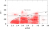 |
Fig. 1 Main asteroid belt plotted in semimajor axis a vs. inclination I. The six defined regions are Inner, Middle, Pristine, Outer, Cybele, and High-Inclination, which are separated by the positions of the major resonances in the asteroid belt. The resonances considered are ν6, 3:1, 5:2, 7:3 and 2:1. The curve denoting the bond of the ν6 resonance was plotted according to Morbidelli & Vokrouhlický (2003). Data were obtained from the Minor Planet Center. |
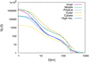 |
Fig. 2 Observed SFDs N(>D) of the six regions of the MB (Cibulková et al. 2014). |
Intrinsic collisional probabilities Pimp and mutual impact velocities vimp between bodies belonging to the different regions of the MB (Cibulková et al. 2014).
3 The model
We built a FORTRAN code, ACDC, based on the prescriptions of the BOULDER code developed by Morbidelli et al. (2009) and the adaptation to six populations made by Cibulková et al. (2014).
ACDC is a multi-population code that simulates the collisional and dynamical evolution of the MB by evolving in time the incremental number of bodies of size D (N(D, t)) in each one of the defined regions. Such evolution, summarized in Eq. (1), is determined by the change in the number of bodies due to the objects being destroyed and fragments being ejected in collisions (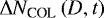 ), which can be positive or negative, and by the dynamical depletion of the MB by the Yarkovsky effect (
 ), which we assume to be negative following the approach of Bottke et al. (2005a), O’Brien & Greenberg (2005), and de Elía & Brunini (2007). ACDC is a statistical code, as it involves a random number generator and Poisson statistics, and so different seeds produce different results.
 (1)
(1)
The ACDC code uses a set of fixed discrete logarithmic size bins. In particular, we used 135 size bins for this work, with central values in the range 1 mm ≤ D ≤ 980 km in diameter in such a way that from one bin to the next the diameter increases by a factor of 101∕15.
In this section, we describe the model and all the methods and algorithms implemented in this work.
Parameters of the scaling law for monolithic basaltic targets and impact speeds of 5 km s−1, derived by Benz & Asphaug (1999).
3.1 Asteroid disruptions – scaling law
The scaling law is a key issue in the model of asteroid collisions, as it dictates the outcome of the impact event. It is determined by the specific energy  , which is defined as the energy per unit mass required to catastrophically disrupt an asteroid (i.e., such that half of the mass is dispersed).
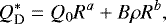
Benz & Asphaug (1999) derived a functional form for the scaling law using SPH simulations for basaltic and icy targets in different impact speeds, given by:
 (2)
(2)
where R is the target radius in centimeters (cm), ρ the target density in g cm−3, Q0 and B normalization parameters, and a and b the slopes of the corresponding power law.
The scaling law that has been used so far in most collisional evolution works of the MB is the one derived by Benz & Asphaug (1999) for monolithic basaltic targets at 5 km s−1 impact speeds. However, using the same law for all the bodies in the asteroid belt implies the assumption that all bodies have the same composition and collide with the same velocities. Previous works attempted to obtain scaling laws for different materials. For example, Cibulková et al. (2014) constructed new  functions for rubble piles using the results of Benavidez et al. (2012), who ran a set of SPH simulations of disruption of D = 100 km rubble-pile targets. However, Cibulková et al. (2014) found that monolithic asteroids provide a better match with the observed data than rubble-piles. Bottke et al. (2005a) and Cibulková et al. (2014) also tested many different scaling laws by changing the exponent b in Eq. (2), and concluded that laws much different from that of Benz & Asphaug (1999) cannot be used for the MB because they fail to reproduce the observed asteroid families.
In our simulations, we therefore decided to use the same  scaling law for all the objects in the MB, namely that derived by Benz & Asphaug (1999) for basaltic materials at 5 km s−1 impact speeds. The values of the parameters involved in the calculation of
  are listed in Table 2.
3.2 Outcome of a single collision
Here, we present the model used to describe the outcome of a single collision between two bodies, which is based on the prescriptions of the BOULDER code (Morbidelli et al. 2009).
We name the bigger body the target, or the parent body, with mass mi, and the smaller body the projectile, or impactor, with mass mj. We assume that all bodies are spherical with uniform density ρ.
After an impact event, fragments are ejected into space. The largest of these fragments has a mass MLF. The SFD of the fragments is represented by a cumulative power law, given by:
 (3)
(3)
where D is the fragment diameter, q a given slope, and A an appropriate normalization constant, considering that there is only one largest fragment after the collision. The largest surviving body after the collision is called the largest remnant, with mass MLR.
The kinetic energy of the impact is the fundamental quantity that determines the outcome of the collision. In particular, we use the specific impact energy of the projectile Q, given by:
 (4)
(4)
where vimp is the impact velocity. The values of vimp are listed in Table 1.
We compare the specific impact energy with the scaling law  (Eq. (2)) and consider two impact regimes:
-
If
 , we have a cratering event. The target ejects fragments into space and a crater is created in the surface of the target.
 -
If
 , we have a catastrophic disruption event, in which more than half of the total initial mass is dispersed in the form of fragments.
The expressions for MLR and MLF derived by Benz & Asphaug (1999) and Durda et al. (2007) are:
![Mathematical equation: \begin{equation*} M_{\text{LR}}=\begin{cases} \left[-\frac{1}{2}\left(\frac{Q}{Q_{\text{D}}^{*}}-1\right)+\frac{1}{2}\right]\left(m_{i}+m_{j}\right), & Q<Q_{\text{D}}^{*} \text{ (cratering)}\\[6pt] \left[-\frac{7}{20}\left(\frac{Q}{Q_{\text{D}}^{*}}-1\right)+\frac{1}{2}\right]\left(m_{i}+m_{j}\right), & Q \geq Q_{\text{D}}^{*} \text{ (catastrophic)} \end{cases}\end{equation*}](/articles/aa/full_html/2020/07/aa37458-20/aa37458-20-eq14.png) (5)
(5)
and
![Mathematical equation: \begin{equation*} M_{\text{LF}}=8\times10^{-3}\left[\frac{Q}{Q_{\text{D}}^{*}}\exp\left(-\left(\frac{Q}{4Q_{\text{D}}^{*}}\right)^{2}\right)\right]\left(m_{i}+m_{j}\right). \end{equation*}](/articles/aa/full_html/2020/07/aa37458-20/aa37458-20-eq15.png) (6)
(6)
If MLR is negative, we assume that the target is pulverized and all mass is lost below the smallest bin.
The slope of the SFD of the fragments is given by:
 (7)
(7)
Since such a steep slope can lead to an unrealistic infinite mass, we assume that the fragment size distribution has a cumulative slope q = −2.5 (Dohnanyi 1969) below a turn-over diameter Dt. We compute Dt so that the mass integral of the fragments is equal to the total ejected mass.
3.3 Collisional evolution
Here, we describe the method used to simulate the collisional evolution of the MB, which consists in modifying the incremental number of objects in every size bin during each timestep. The total integration time is 4000 Myr.
We split the MB in six regions of index r, where r = 1,..., 6. i and j denote the target and projectile indexes, with diameters Di and Dj and belonging to populations ri and rj, respectively.
Before the simulation starts, we arrange two quantities for all possible target–projectile pairs: the frequency of each possible collision and their outcomes. The first is given by:
 (8)
(8)
where the values of the intrinsic impact probabilities  are listed in Table 1 (Cibulková et al. 2014).
Following the algorithm outlined by O’Brien & Greenberg (2005), we generate 3D arrays  , where k is the size bin. These arrays give the incremental fragment SFD resulting from every possible collision derived from Eq. (3). The F arrays are symmetrical between targets and projectiles, and hence between regions, since the collision probabilities and impact velocities are the same regardless of which body is the target or projectile. We create one array for every pair of regions and the number of F arrays created in this six-region model is 21.
At this point we begin the simulation. First, we calculate the integration time step Δt. To do so, we calculate the collisional lifetimes  of all asteroids from all regions, by summing all the projectiles that can catastrophically disrupt them:
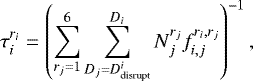 (9)
(9)
where  is the incremental number of projectiles and
  the diameter of the smallest projectile that can catastrophically disrupt the target.
The timestep Δt is therefore calculated as ten times smaller than the minimum  value. By doing so, we assure that, from one timestep to the other, the removal of bodies in a size bin never exceeds 10%.
The change in the number of bodies of a given size is determined by two quantities: the number of collisions, and the outcome of each event (i.e., bodies destroyed and fragments created).
We calculate the deterministic number of collisions between all target–projectile pairs in the six regions of the MB:
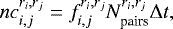 (10)
(10)
where  is the number of target-projectile pairs, which is determined by
  and
and  , the number of targets and projectiles of diameter Di and Dj, respectively.If both target and projectile belong to the same size bin and population, their numbers are equal, and so the number of pairs is given by:
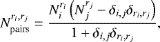 (11)
(11)
where the δ function is the Kronecker delta.
If any number of collisions between a given target–projectile pair is smaller than a limit value of 5, we recalculate it with Poisson statistics using the result given by Eq. (10) as the mean value and a random seed (Press et al. 1992). Therefore, in a given timestep, the number of collisions can be an integer number between 0 and 5.
Next, we calculate the change in the number of bodies of a given size bin k in a region r by taking into account all of the bodies destroyed as well as the new fragments created:
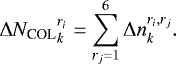 (12)
(12)
If both target and projectile belong to the same region, the change is simply given by the number of collisions multiplied by the number of fragments created in each bin; however, if they belong to different regions, mixing between targets and projectiles from the distinct regions must be considered by removing projectiles from one region and adding them to the other. The expressions of the interaction terms, which were adapted from O’Brien & Greenberg (2005), are given by:
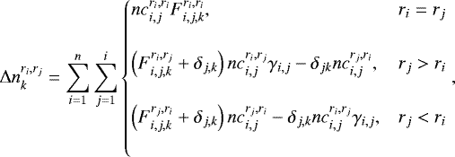 (13)
(13)
where we name γi,j = 1 − δi,j and n is the number of size bins.
Since our model deals with a finite number of bins, the bodies able to disrupt the smallest bodies are generally smaller than the first bin.Ignoring the disruption of the smallest bodies may lead to unrealistic waves in the size distribution (Campo Bagatin et al. 1994; Durda & Dermott 1997). In order to prevent these undesirable artificial waves, we do not calculate the collisional evolution of the bodies smaller than 10 cm; instead, we extrapolate them from the larger bodies after each timestep.
3.4 Dynamical evolution: Yarkovsky effect
The Yarkovsky effect is a radiation force that produces the change in the orbital parameters of small rotating asteroids because of the asymmetry between the direction of absorption of sunlight and the direction of re-emission of thermal radiation. The radiated energy causes a force along the body’s orbit that in turn causes asteroids smaller than tens of kilometers to slowly drift in semi-major axis, allowing them to reach resonances with the planets that drive them into planet-crossing orbits. Thus, the Yarkovsky effect causes a dynamical depletion of the MB, and can be considered a “sink” for small asteroids. This depletion affects the collisional evolution of the MB, because fewer smaller bodies means fewer collisions with larger bodies, and therefore it has to be considered in any collisional evolution model.
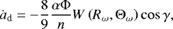
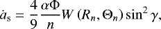
The general expressions for the diurnal and seasonal Yarkovsky effects are (Peterson 1976; Burns et al. 1979; Rubincam 1995; Vokrouhlicky 1998; Farinella et al. 1998; Vokrouhlický & Farinella 1999; Vokrouhlický et al. 2015):
 (14)
(14)
 (15)
(15)
where α = 1 − AB, AB denoting the Bond albedo (Vokrouhlický & Bottke 2001),  , with R being the radius of the body, F the solar radiation flux at the orbital distance a from the Sun, m the mass of the body, c the speed of light, n the orbital mean motion, ω the rotation frequency, and γ the spin-axis obliquity.
The function  depends on parameters like the thermal conductivity K, the thermal capacity C, the density ρ, and a frequency ν, which is equal to n for the seasonal effect and ω for the diurnal effect. It is determined by the radius of the body R, which is scaled by the penetration depth
  of the thermal wave, and the thermal parameter
  . The function W is given by:
 (16)
(16)
The expression for the seasonal effect (Eq. (15)) is accurate for bodies bigger than 4lν (Farinella et al. 1998). We assume that for bodies smaller than 4lν, ȧs ∝ D3∕2 (O’Brien & Greenberg 2005).
In the thermal model, following Cibulková et al. (2014), we assume a break in the thermal conductivity that reflects the rotational parameters of small bodies (Warner et al. 2009): K = 0.01 W m−1 K−1 for D > DYE and K = 0.01 W m−1 K−1 for D ≤ DYE. We assume the value of the transition value DYE = 200 m and a size-dependent spin rate  , P0 = 5 h, D0 = 5 km. The thermal capacity assumed is C = 680 J kg−1 K−1, the infrared emissivity ɛ = 0.95, and the Bond albedo AB = 0.02. As the diurnal and seasonal effects depend on cosγ and sinγ, respectively, we consider a mean obliquity of 45° in order to calculate a mean Yarkovsky effect. The physical densities considered for the bodies of the different regions of the MB are shown in Table 3.
Following Cibulková et al. (2014), we assume that the Yarkovsky effect causes an exponential decay described by:
 (17)
(17)
where  is the number of bodies of diameter D from region r at time t, and Δt is the timestep. In particular,
  is the characteristic timescale of the Yarkovsky effect, which is defined as the mean time it takes for asteroids to reach a resonance:
 (18)
(18)
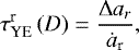
where Δar is half of the region size in semi-major axis (see Table 3), and ȧr is the sum of the rates associated with the diurnal and seasonal Yarkovsky effects calculated with Eqs. (14) and (15), respectively. The values of ȧ as a function of size, for the diurnal, seasonal, and total Yarkovsky effect are plotted for each region in Fig. 3. We find a total drift rate of 1− 3 × 10⁻⁴ AU Myr−1 for 1 km bodies, a range that contains typical values of 2 × 10⁻⁴ AU Myr−1 (Granvik et al. 2017). The timescales for the six regions are plotted in Fig. 4, which are consistent with the ones derived by Cibulková et al. (2014).
In summary, the total number of bodies removed from a region due to the Yarkovsky effect to be included in Eq. (1) is  . It is important to note that this general dynamical model, formulated as it is, assumes two things: when asteroids fall into resonances, they are immediately removed from the MB and added to the NEA region, and all resonances remove asteroids with the same efficiency. However, since the timescale depends on the size of the region (Δa in Eq. (18)), we observed that the timescale for the Pristine region is very short, and causes an excessive depletion in this region, which is narrower and less populated than the other regions. Gladman et al. (1997) studied the dynamical lifetimes of asteroids injected into the resonances and calculated the time it takes to cross the orbit of Earth. These latter authors found times shorter than 1 Myr for strong resonances, like ν6, 3:1J and 5:2J. However, they found that if an asteroid falls into the 7:3J resonance, which is the one that separates the Pristine from the Outer belt, it takes ~6.3 Myr to cross Earth’s orbit. Taking this particular feature of the Pristine belt into consideration in our general Yarkovsky model, we found that we can counter the excessive dynamical depletion and make a better fit with observations if we multiply the timescale of the Pristine region by a factor of three. By doing this, we enable the asteroids that fall into the 7:3J resonance to stay in the Pristine region for a longer time before being removed from the asteroid belt. It is worth noting that our solution found for Pristine takes into account the many uncertainties involved in a general Yarkovsky model, as well as the particular characteristics of that region.
Parameters of the Yarkovsky effect for the different regions of the MB (Cibulková et al. 2014).
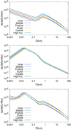 |
Fig. 3 Semimajor-axis drift rate ȧ due to the Diurnal (top), seasonal (middle), and total (bottom) Yarkovsky effect as a function of size, for the six regions of the MB. |
 |
Fig. 4 Timescale τYE of the Yarkovsky effect as a function of size D for the six regions of the MB. The black line indicates the total integration time of 4000 Myr. |
3.5 Fit with observational data
As mentioned above, the code developed in this work is a statistical model that treats big impacts as random events using Poisson statistics. Therefore, runs using different seeds for the random number generator produce different results, and so we develop a set of runs using different random seeds and then interpret the results statistically.
To obtain a quantitative measure of how well a simulation reproduces observational data, we follow the procedure described by Bottke et al. (2005b) and Cibulková et al. (2014). The metric used to determine the goodness of fit between the observed size distribution of a region (Nobs) and the simulation results (Nsim) is a hybrid ψ2 test:
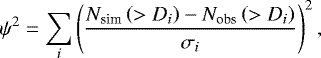 (19)
(19)
where the summation extends over a range of diameters Dmin (~3–6 km) and Dmax ~ 250 km, estimated from the observed SFDs (Cibulková et al. 2014). The uncertainties are given by  . For each run, we calculate the individual metrics
  for the six regions and then a global metric
  for the MB as a whole, and also a mean metric
  , by simply averaging the metrics of the six regions.
The ideal case is to find a set of runs that produce good fits in the individual regions and globally. However, this is very unlikely to happen in a single run due to the high stochasticity and randomness of big impact events and the mutual interactions between the different regions of the MB. It is possible that some runs may produce good fits in some populations and simultaneously bad fits in other populations. Also, some runs may produce bad fits in individual populations, but produce a good match with the global MB. Moreover, some runs can even produce impossible results like Vesta colliding with Ceres and thus destroying the most massive bodies in the asteroid belt. Therefore, a very low number of acceptable runs is expected. The criterion adopted in this work is to select runs by sorting the ones with the lowest  metrics and then calculate medians of the desired results.
4 Dynamical evolution of the NEAs
In this section, we present our modeling of the dynamical evolution of the NEAs. The asteroids that escape from the MB due to the combined action of the Yarkovsky effect and resonances are delivered to the NEA population (e.g., Gladman et al. 1997; Bottke et al. 2002; Granvik et al. 2016). The asteroids in Earth-crossing orbits reside in that region for some time until they reach a sink. The most important sinks of NEAs are collisions with the Sun, escape from the inner Solar System after a close encounter with Jupiter (Granvik et al. 2018), destruction by thermal effects (Granvik et al. 2016), and collisions with terrestrial planets. It was shown by Bottke et al. (2002) and Granvik et al. (2018) that the different entrance routes yield different mean lifetimes. The different regions of the MB that we take into accountin this work are bounded by the resonances that Granvik et al. (2018) consider as entrance routes. Therefore, asingle region of the MB can deliver asteroids to the NEA population through different entrance routes.
Based on our partition of the MB (see Fig. 1), we consider the ν6 and 3:1J resonances as the entrance routes for the NEAs coming from the Inner belt, 3:1J and 5:2J for those coming from the Middle belt, 5:2J and 2:1J for those coming from the Pristine and Outer belts, 2:1J for those coming from the Cybele belt, and 3:1J, 5:2J, 2:1J, and Phocaeas for those coming from High-Inclination belt (Granvik et al. 2017).
In orderto quantify the contribution of the different regions of the MB to the NEAs, we calculate the mean dynamical lifetimes of NEAs according to their source regions. To do so, for each of our regions we average the lifetimes of bodies τ, weighted by the contribution of NEAs coming from each of the surrounding resonances. In particular, we use the values for the average lifetimes L in the NEA region and the prediction for the debiased number of NEAs coming from each of the resonances derived by the dynamical simulations performed by Granvik et al. (2018), listed in Table 4. Thus, we calculate the mean lifetimes of NEAs coming from the given regions as follows:
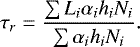 (20)
(20)
We split the number of NEAs N that are delivered through a resonance according to the contribution from each region. The values α in Eq. (20) represent, for each resonance, the fraction of N that comes from the adjacent regions. For example, we consider α = 0.5 for 3:1J, which means that half of the bodies that enter in the NEA region via the 3:1J resonance are delivered by the Inner belt while the other half is delivered by the Middle belt, as was proposed by Bottke et al. (2002). Similarly, as our High-Inclination belt contains all asteroids in the MB with inclinations greater than 20°, we split N according to h, the fraction of NEAs that enter a resonance from a low or high inclination region. For example, we assume h = 0.8 for 3:1J, which means that 80% of bodies come from inclinations smaller than 20° while 20% come from inclinations greater than 20°. We estimated these fractions with the simulations performed by Granvik et al. (2017). The values we assumed for the α and h fractions are listed in Table 5.
The Pristine and Outer belt are limited by 5:2J, 7:3J, and 2:1J, but the effect of 7:3J is not clear from the dynamical simulations of Granvik et al. (2017, 2018). Moreover, it shows that the asteroids from the Outer belt are able to cross the 7:3J resonance and enter the Pristine region, a process we are not considering in this model. Thus, we assign the same time to the Outer, Pristine, and Cybele regions by averaging the times of 5:2J and 2:1J, with Eq. (20).
The High-Inclination region in our collisional model spans the entire MB in semi-major axis, and therefore passes through all the major resonances present there, each having different associated lifetimes as Table 4 shows. Therefore, we split the contribution of the High-Inclination from our model into three different subregions corresponding to the Inner, Middle, and Outer ranges in semi-major axis. We assign them 80, 5, and 15% of the High-Inclination contribution, respectively, consistent with the outputs of the simulations performed by Granvik et al. (2017), and calculate their dynamical times separately with Eq. (20).
Table 5 summarizes the mean dynamical times for NEAs coming from the different regions of the MB, calculated with Eq. (20), as well as the way we group the contribution for each resonance.
However, there could be different mechanisms capable of delivering larger asteroids. In fact, the numerical simulations performed by Migliorini et al. (1998) show that weaker resonances in the inner belt dominate the delivery process for large asteroids, asthey can cause asteroids to increase in orbital eccentricity to Mars-crossing values. These weaker resonances were studied by Nesvorný & Morbidelli (1998) and Morbidelli & Nesvorný (1999). Following O’Brien & Greenberg (2005) and de Elía & Brunini (2007), we treat the dynamical removal of NEAs larger than 5 km from the Inner and Middle belts using a dynamical lifetime of 3.75 Myr, which is the lifetime associated with the Mars-crosser population (Bottke et al. 2002).
We then calculate the number of NEAs in time, coming from a region of the MB, as (O’Brien & Greenberg 2005):
 (21)
(21)
where the second term represents the number of bodies delivered from the MB via the combined action of the Yarkovsky effect and resonances at the time t, and the third term is the dynamical removal of NEAs. We do not consider the Yarkovsky effect in the NEA population. In fact, the Yarkovsky effect on the orbits of the NEAs is many orders of magnitude lower than the gravitational perturbations made by the close encounters with terrestrial planets (Granvik et al. 2018). We also do not consider collisions between NEAs and other asteroids.
Prediction for the debiased number of NEAs N coming from each entrance route in the range 17 < H < 25, and average lifetime in the NEA region L (Granvik et al. 2018).
Mean dynamical lifetimes of NEAs coming from the different regions of the MB, calculated according to the parameters listed in Table 4 (Granvik et al. 2018), the simulations performed by Granvik et al. (2017), and Eq. (20).
5 Results
In this section, we present the results of the simulations we performed with the ACDC code. First we describe how we arrive at a satisfying set of initial conditions. Then, we show the final SFDs of the six regions of the MB. Finally, we derive the HFD of the NEAs and find the contribution of the six regions of the MB to the NEAs.
5.1 Finding the initial conditions
The initial conditions in our simulations are the SFDs of the six regions of the MB, which were constructed as three-slope cumulative power laws:
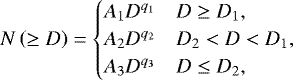 (22)
(22)
where the free parameters are the cumulative slopes q1, q2, and q3, the cut-off diameters D1 and D2, and the normalization constants A1, A2 and A3.
We manually added the parental bodies of observed asteroid families with DPB > 100 km and MLR∕MPB < 0.5, which cannot be completely destroyed by collisional evolution (Bottke et al. 2005a) or by the Yarkovsky effect (Bottke et al. 2001). We used the parent body diameters estimated by SPH simulations by Durda et al. (2007), which were summarized by Brož et al. (2013), and are listed in Table 6. We calculated mean values in the cases where the estimation takes a widerange of values. In the case of Polana, an asteroid family located in the Inner belt for which there is no available estimation of its parent body size due to its complex structure (Walsh et al. 2013; Dykhuis & Greenberg 2015), we considered a parent bodysize of 115 km, which is consistent with the parent body sizes of other families in the Inner belt. We also manually added the three biggest asteroids: Vesta in the Inner belt, Ceres in the Middle belt, and Pallas in the High-Inclination belt.
Cibulková et al. (2014) performed a detailed exploration of this free-parameter space in a wide range of slopes and cut-off diameters, and found a set of values that give their best fit with observational data. However, it is very important to note that the main simulations in their work did not include the Yarkovsky effect. By considering the radiation force, the main consequence is a depletion of bodies in the subkilometer range. We found it necessary to use steeper initial slopes and higher cut-off diameters in order to account for the dynamical removal of bodies and reproduce the observed distributions.
For the construction of our initial conditions for the SFDs, we explored a wide range of slopes and cut-off diameters by trial and error. The method we used for this exploration is to perform a set of runs for each set of parameter values in order to search for the ones that give lower simultaneous metrics and median SFDs as close as possible to the observed data. The set of initial populations tested, including the one chosen for this work, is plotted in Fig. 5. The slopes and cut-off diameters of the initial conditions used in this work are listed in Table 7.
Asteroid families in the individual parts of the MB according to Brož et al. (2013).
Input parameters chosen for the initial cumulative size frequency distributions of the six parts of the MB.
5.2 Mainbelt
Here, we describe the results of the 2500 runs that we performed using our six-region collisional evolution model regarding the six regions of the MB. The cumulative distributions of the ψ2 metrics of the six regions, along with the global MB  and the averaged metric
  of the performed runs are plotted in Fig. 6. We find that all of our runs produce good fits with the global MB. In fact, all of our runs produce
  between 5 and 75, and 10% of runs produce global metrics smaller than 20. The individual metrics give a wider range of values. The lowest metrics of the individual regions lie between 10 and 25. The regions that produce the lowest metrics are the Cybele and High-Inclination belts, while the Inner and Middle belts give the highest metrics. However, it is worth remembering that, in general terms, not all regions give low metrics simultaneously in a single run. The mean metrics
  , which were calculated by averaging the individual metrics in each run, show values between 80 and 100 and smaller than 120 in 1 and 10% of cases, respectively. For our analysis, we select the runs that give mean metrics
  smaller than 100, which is 1% of the total.
Our results concerning the formation of asteroid families in the MB is plotted in Fig. 7. We reiterate the fact that we only consider asteroid families produced by the catastrophic disruption of parental bodies bigger than 100 km, such that MLR∕MPB < 0.5. Our runs produce a wide number of families, but the median is a good match with the actual observed families. Specifically, the median values lie within the uncertainties, which are calculated as the square root of the observed number of families. The only exception is the High-Inclination region, which has one observed family while our runs produce three families in median.
The resulting SFDs of the selected runs of the six regions of the MB, along with the median SFDs are plotted in Fig. 8, while the SFD for the global MB is plotted in Fig. 9. In general terms, we see that our selected runs provide very good fits with the observed data for the six regions and the global MB. Specifically, the results for the Inner, Middle, Pristine, and Outer regions lie in a narrow dispersion along the observed data, while the Cybele and High-Inclination belts show the greatest dispersion between the different runs. We find that the simulations that produce no families in the Cybele region are the ones that produce better fits with observed data.
We find two discrepancies worthy of mention. One is regarding the tail of small bodies of the Inner belts, which is shallower than the observed data. This was also noted in the work of Cibulková et al. (2014). To explain this small body deficit of the Inner belt, these latter authors proposed the recent disruption (during the last 100 Myr) of a large parent body that made the actual SFD temporarily steep. An alternative explanation is that the Yarkovsky model in the Inner belts could be making small asteroids drift too quickly. This may be solved in future works by including YORP cycles that result in a slower net Yarkovsky drift, as was shown by Bottke et al. (2015) and Granvik et al. (2017). The other discrepancy is in the bigger objects of the Outer belt, and is due to the formation of asteroid families. We reiterate the fact that in the construction of the initial conditions, we manually added the estimated parental bodies of the observed asteroid families (Brož et al. 2013). In the case of the Outer belt, these parental bodies have diameters between ~100 and ~400 km. We find that our runs reproduce the number of observed families, as shown in Fig. 7. However, the parental bodies that are catastrophically disrupted are mostly smaller than the ones we considered beforehand. This discrepancy may be a consequenceof using the same scaling law throughout the entire MB. It was shown in Cibulková et al. (2014) that the formation ofasteroid families depends on the scaling law, and that there could be different scaling laws for different parts in the MB due to the diverse compositions of asteroids (DeMeo & Carry 2014). The use of weaker scaling laws in the Outer belt, such as for example the laws for ice in Benz & Asphaug (1999), may enable a wider range of projectiles capable of catastrophically disrupting these large bodies, increasing the probability of the occurrence of such events, and thus improving the results at the large end. The treatment of these discrepancies represents an interesting starting point for future research.
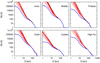 |
Fig. 5 Initial SFDs tested for the six populations of the MB are shown by red lines. Blue lines denote the observed SFDs, while the black lines denote the chosen initial SFDs for this work. |
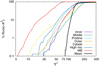 |
Fig. 6 Cumulative percentage distribution of ψ2
metrics. We plot ψ2
for the six regions of the MB, including a metric for the global MB |


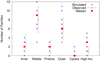 |
Fig. 7 Number of families formed in the individual regions, out of the catastrophic disruption of parent bodies bigger than 100 km and MLR∕MPB < 0.5. The error bars denote the uncertainties of the observed numbers of families, calculated as the square root of the observed number of families. |
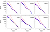 |
Fig. 8 Size–frequency distributions of the six regions of the MB. The selected runs and their median are plotted in purple and black lines, respectively. The observed SFDs are plotted in blue and the initial SFDs are plotted in red. |
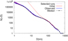 |
Fig. 9 Size–frequency distributions of the global MB, calculated as the sum of the SFDs of the individual regions. The selected runs and their median are plotted in purple and black lines, respectively. The observed SFD is plotted in blue and the initial SFD is illustrated in red. |
5.3 Near-Earth asteroids
Here, we proceed to describe the results of our simulations for the NEAs. We proceed, as described in Sect. 4, to calculate the evolution of the NEA populations by considering the asteroids delivered via Yarkovsky effect and resonances, and the dynamical remotion due to the many sinks present in the inner Solar System. By doing so, we obtain the current size distribution of NEAs coming from the different source regions.
Because our simulations originally deal with size bins, we convert the diameters into absolute magnitudes H using the relation (Bowell et al. 1989):
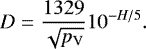 (23)
(23)
This relationship depends on pV, the visual geometric albedo, which is likely size dependent. Indeed, it was suggested by Mainzer et al. (2014) that there is an increase in albedo with decreasing diameter. In this work, we consider the values pV = 0.11 for D > 3 km and pV = 0.15 for D < 3 km, which are consistent with the measures of Mainzer et al. (2014).
Recently, Granvik et al. (2018) developed a model of the NEO population that derived a debiased steady-state distribution of orbital elements and absolute magnitudes H in the range 17 < H < 25 (1.4 km > D > 35 m, for pV = 0.15). The cumulative magnitude-frequency distribution derived by Granvik et al. (2018) in the range of absolute magnitudes 17 < H < 25 is shown in Fig. 10. It should be noted that the observed population is thought to be complete up to H < 16 (~ 2 km for pV = 0.15) (Tricarico 2017). Figure 10 shows the total derived NEA population along with the observed NEA population obtained from the Minor Planet Center2. We also plot the recent HFDs derived by Harris & D’Abramo (2015) and Tricarico (2017) for comparison. We find that our median magnitude distribution provides a good match with observations in the range of completeness, H < 16. The estimated magnitude distribution agrees with recent works in the range 16 < H < 20 (~ 2 km > D > 350 m, for pV = 0.15), but deviates significantly in H > 20. The main difference is that our median distribution has a change to a steeper slope around H ~ 21 (~ 220 m for pV = 0.15), while Granvik et al. (2018) and Harris & D’Abramo (2015) find a dip in the population in the range 19 < H < 25 (550 m > D > 35 m, for pV = 0.15). The immediate consequence of this change to a steeper slope in our median magnitude distribution is a higher number of smaller NEAs. Moreover, our work predicts ~107 asteroids with H < 25 (35 m, for pV = 0.15), which is an order of magnitude higher than the ~106 asteroids of that size made by previous papers. This is most likely caused by the many uncertainties and free parameters regarding the modeling of the Yarkovsky effect, and the exclusion of YORP cycles, especially for smaller asteroids. More specifically, bodies of ~ 10 m in size have the lowest timescales associated with the Yarkovsky effect, as shown in Fig. 4. As a consequence, this results in a larger number of asteroids delivered to the NEA region. However, since the MB is not complete in the subkilometer range, smaller asteroids are far outside of the observational constraints that we are able to use in this collisional model. Therefore, we limit our analysis to the kilometer range, and will investigate how we can extrapolate results for asteroids bigger than 100 m.
We now proceed to studying the contribution of the different regions of the MB to the NEAs. The left panel of Fig. 11 shows the percentages of NEAs coming from the different regions of the MB, which were calculated with respect to the total cumulative number of NEAs we obtained in our simulations. We find that all regions contribute to the NEA population to a greater or lesser extent. The regions that make the smallest contributions are the Pristine and Cybele belts. In fact, these regions beyond the 5:2J resonance provide less than 4 and 1% of the NEAs, respectively, in sizes smaller than 5 km. The regions that make the biggest contributions are the Inner and Middle belts, which together account for ~ 60% of small NEAs, providing ~27 and ~32% of bodies bigger than 1 km, respectively, while the Outer belt provides ~ 18%. We see that the percentages remain similar in smaller sizes. We obtain that the High-Inclination belt is the source of ~ 17% of NEAs larger than 1 km. In our partition of the MB, the High-Inclination region is made of all the asteroids with inclinations greater than 20°, spanning the entire MB in semi-major axis. Thus, the High-Inclination region contains asteroids that could be assumed to be part of the Inner, Middle, and Outer belts if we consider the whole range of inclinations. If we redistribute the contribution of the High-Inclination region into the Inner, Middle, and Outer belts with respect to the way these are defined in Sect. 4, and adding the Pristine and Cybele NEAs as part of the Outer region, we see in the right panel of Fig. 11 that the results change, as follows: we find that ~ 77% of the NEAs come from the Inner and Middle belts, which provide ~44 and ~33%, respectively, and ~23% come from the Outer belt. These values are valid for NEAs bigger than 1 km spanning the whole range of inclinations,but we see in Fig. 11 that the percentages remain similar in smaller sizes. In the multikilometer range, the Inner belt is the main source of NEAs, as the right panel in Fig. 11 shows. We note that the share of Outer belt NEAs slightly increases, matching the Middle belt contribution in ~ 3 km. However in larger size ranges, as is explained below, the number of NEAs becomes too small for this to be taken as a strong statistical result.
The top and bottom panels of Fig. 12 show the number of NEAs bigger than 1 km and 5 km, respectively, according totheir source regions; the total numbers we obtain in our simulations are 1002 and 26, respectively. We find that the Inner regionprovides 432 NEAs bigger than 1 km, out of which 277 come from the proper Inner belt, while 158 come from the corresponding section of the High-Inclination region. Similarly, 323 NEAs come from the Middle belt with 9 from the Middle High-Inclination region. The Outer region and Outer High-Inclination belt provide 186 and 8 NEAs bigger than 1 km, respectively, while the Pristine and Cybele belts provide 31 and 12, respectively. The bottom panel of Fig. 12 shows that the Middle and Outer belts provide 8 and 7 NEAs bigger than 5 km, respectively.We see that the High-Inclination region does not provide large NEAs corresponding to the Middle and Outer belts,and neither the Pristine nor Cybele belt provides any NEAs in this size range. Moreover, we find that, out of the 11 NEAs bigger than 5 km that come from the Inner part, 6 came from the High-Inclination belt.
It is interesting to compare the results concerning NEAs coming from the High-Inclination belt with the actual observed distribution of NEAs with high inclinations (i.e., i > 20°). As we show in Fig. 11, the percentage of NEAs bigger than 1 km coming from the High-Inclination belt is ~ 17%. However, by exploring the MPC database, we find that ~108 NEAs with H < 16 (the complete population) have orbital inclinations i ≳ 20°, which is ~ 56% of the total number of NEAs with H < 16. The existence of high-inclination NEAs coming from a source other than the High-Inclination belt is something this study is not able to explain as we do not calculate the evolution of the orbital elements. However, the simulations performed by Granvik et al. (2016, 2018) show that there are dynamical processes that modify the inclinations of asteroids when leaving the MB. In particular, Granvik et al. (2016) show that 3:1J, 5:2J, and 7:3J resonances, and especially the 2:1J resonance, are able to deliver low-inclination asteroids to the NEA region with inclinations beyond 20°. Moreover, these mean-motion resonances can also decrease inclinations in such a way that asteroids that initially had high inclinations enter the NEA region with inclinations smaller than 20°. Furthermore, Granvik et al. (2018) show that NEAs delivered from these latter four resonances and also from ν6 and 3:1J are able to increase their inclinations inside the NEA region through dynamical evolution. Therefore, the High-Inclination belt is not necessarily the source of NEAs with large inclinations. Moreover, the High-Inclination belt is the source of only a fraction of the observed NEAs with high inclinations, while the rest increased their inclinations through dynamical evolution.
It is interesting to compare our results regarding the proportions of NEAs from different source regions with previous works. However, comparisons between collisional and dynamical simulations of the MB must be handled with care. Indeed, it is not yet possible to address the collisional and fragmentation processes simultaneously with the dynamical evolution in the MB in a self-consistent way, and therefore some differences are expected.
Bottke et al. (2002) found that ~60% of NEOS come from the Inner belt, ~25% from the Middle belt, ~8% from the Outer belt, and ~6% for the Jupiter-family Comets, which we do not consider here. The contribution from the Outer belt in our work, adding the NEAs provided by the Pristine, Cybele, and the corresponding fraction of High-Inclination, is ~ 25%. However, the lifetime in the NEA region of bodies from the Outer belt found by Bottke et al. (2002) is 0.14 Myr, much smaller than the value derived in our work by averaging the lifetimes of 0.68 Myr and 0.4 Myr, associated with the 5:2J and 2:1J resonances, respectively (Granvik et al. 2018). If we use the time of 0.14 Myr for the Outer belt, we find that the percentages of the total NEAs found in the Inner, Middle, and Outer belts are ~ 50, ~ 40, and ~ 10% respectively, which are closer to the percentages found by Bottke et al. (2002). However, using this latter lifetime for the Outer-belt NEAs results in a HFD that does not match the observed data.
It was shown by Granvik et al. (2018) that ν6 is the resonance that provides the highest number of NEAs throughout the whole size range, followed by 3:1J, which immediately results in a dominance of the Inner belt as the main source of NEAs. As shown above, we are able to obtain a similar result when we redistribute the contribution of the High-Inclination region between the Inner, Middle, and Outer NEAs.
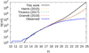 |
Fig. 10 HFD of the NEA population. The median distribution calculated in this work is plotted in black. The observed NEAs, taken from the Minor Planet Center, are plotted in blue. Dashed lines indicate the derived HFDs of Harris & D’Abramo (2015); Tricarico (2017); Granvik et al. (2018). |
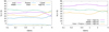 |
Fig. 11 Percentage of NEAs coming from the different regions of the MB with respect to the total cumulative number of NEAs we obtained in the simulations. Left panel: considering the six regions. Right panel: distributing the High-Inclination NEAs among the Inner- Middle-, and Outer-belt NEAs, and adding the Pristine and Cybele contributions to the Outer-belt NEAs. |
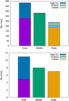 |
Fig. 12 Number of NEAs bigger than 1 km (top) and 5 km (bottom), according to their source regions. The small contributions of the Pristine and Cybele belts are added to the Outer belt, while the High-Inclination NEAs are distributed among the Inner, Middle, and Outer NEAs. |
6 Conclusions and discussion
Here, we present the ACDC code, a six-part collisional and dynamical evolution model of the MB, which we split into six regions according to the positions of the 3:1, 5:2, 7:3, and 2:1 mean-motion resonances with Jupiter and the ν6 secular resonance with Saturn. The six regions we consider, following the previous work of Cibulková et al. (2014), are the Inner, Middle, Pristine, Outer, Cybele, and High-Inclination belts. The ACDC code calculates the evolution in time of the number of objects in each part of the MB due to collisions between the asteroids of the different regions. ACDC is a statistical code, as it treats big impact events with a random number generator and Poisson statistics. It also considers the dynamical depletion of the MB via the Yarkovsky effect, which slowly drifts small asteroids into the resonances and delivers them into the NEA region. We used the ACDC code to derive SFDs of the six regions of the MB, estimate a HFD for the NEAs, and studied the contribution of each region to the NEA population.
The results of this work can be summarized as follows:
-
We find that our six-part collisional evolution model shows a good fit to the observed data in the six regions of the MB, and to the MB considered as a single population. We are also able to reproduce, within the expected uncertainties, the number of observed asteroid families formed from the catastrophic disruption of parent bodies bigger than 100 km. There are two main discrepancies in the resulting SFDs. The first is located at the small end of the SFD for the Inner belt, which may be corrected in future works with a better model of the Yarkovsky effect.The second is related with the largest bodies in the Outer belt, and may be corrected by exploring different scaling laws in that particular region which may enable a wider range of projectiles capable of disrupting these large bodies. The treatment of these discrepancies represents an interesting starting point for future research.
-
We obtain a good fit with the currently observed magnitude distribution of NEAs in the range of completeness, H < 16, and withthe recent estimations in the range 17 < H < 20. Our HFD deviates from previous estimates for smaller bodies. This discrepancy is most likely caused by the many uncertainties and free parameters regarding the current model of the Yarkovsky effect, especially for smaller asteroids. Further studies may require an improved model of the Yarkovsky effect for smaller asteroids, and may also consider the inclusion of the YORP effect, which was not considered here. However, the subkilometer-sized asteroids are out of the available observational constraints for the present collisional model, as the MB is not complete below the kilometer scale.
-
We find that all the regions in the MB contribute to the NEA population to a greater or lesser extent. The most important sources are the Inner and Middle belts followed by the Outer belt. The Pristine and Cybele belts make a very small contribution to the NEAs.
-
It is not possible from this work to address the origin of NEAs with inclinations greater than 20°, as the resonances in the MB and the dynamics in the NEA region are able to increase and decrease the inclinations of the asteroids (Granvik et al. 2017, 2018). The High-Inclination belt can be the source of only a fraction of the currently observed NEAs with large inclinations, while the rest of the NEAs obtained their inclinations through dynamical evolution. Further dynamical studies may be able to provide more clarity on the origin of high-inclination NEAs.
We have improved on previous collisional studies as we have consistently included a general model of the Yarkovsky effect into a six-population collisional evolution model of the MB for the first time. Moreover, our work forms a starting point for further studies and applications regarding the collisional history of the MB, and also any other small-body population in the Solar System. We also obtained the population of NEAs, identifying their proportion from each source in the MB. This is undoubtedly an important contribution concerning the composition and diversity we can expect in such objects.
Acknowledgements
The present investigation work was partially financed by Agencia Nacional de Promoción Científica y Tecnológica (ANPCyT) through PICT 201-0505, and by Universidad Nacional de La Plata (UNLP) through PID G144. We acknowledge the financial support by Facultad de Ciencias Astronómicas y Geofísicas de La Plata (FCAGLP) and Instituto de Astrofísica de La Plata (IALP) for extensive use of their computing resources. We are grateful to Miroslav Brož for kindly providing us the observed data, and to Mikael Granvik (as a reviewer) for valuable comments and suggestions that helped us improve the manuscript.
References
- Benavidez, P. G., Durda, D. D., Enke, B. L., et al. 2012, Icarus, 219, 57 [NASA ADS] [CrossRef] [Google Scholar]
- Benz, W., & Asphaug, E. 1999, Icarus, 142, 5 [NASA ADS] [CrossRef] [Google Scholar]
- Bottke, W. F., & Greenberg, R. 1993, Geophys. Res. Lett., 20, 879 [NASA ADS] [CrossRef] [Google Scholar]
- Bottke, W. F., Vokrouhlický, D., Broz, M., Nesvorný, D., & Morbidelli, A. 2001, Science, 294, 1693 [NASA ADS] [CrossRef] [PubMed] [Google Scholar]
- Bottke, W. F., Morbidelli, A., Jedicke, R., et al. 2002, Icarus, 156, 399 [NASA ADS] [CrossRef] [Google Scholar]
- Bottke, W. F., Durda, D. D., Nesvorný, D., et al. 2005a, Icarus, 175, 111 [NASA ADS] [CrossRef] [Google Scholar]
- Bottke, W. F., Durda, D. D., Nesvorný, D., et al. 2005b, Icarus, 179, 63 [NASA ADS] [CrossRef] [Google Scholar]
- Bottke, W. F., Vokrouhlický, D., Walsh, K. J., et al. 2015, Icarus, 247, 191 [NASA ADS] [CrossRef] [Google Scholar]
- Bowell, E., Hapke, B., Domingue, D., et al. 1989, in Asteroids II, eds. R. P. Binzel, T. Gehrels, & M. S. Matthews (Berlin: Springer), 524 [Google Scholar]
- Brož, M., Morbidelli, A., Bottke, W. F., et al. 2013, A&A, 551, A117 [NASA ADS] [CrossRef] [EDP Sciences] [Google Scholar]
- Burns, J. A., Lamy, P. L., & Soter, S. 1979, Icarus, 40, 1 [NASA ADS] [CrossRef] [Google Scholar]
- Campo Bagatin, A., Cellino, A., Davis, D. R., Farinella, P., & Paolicchi, P. 1994, Planet. Space Sci., 42, 1079 [NASA ADS] [CrossRef] [Google Scholar]
- Cibulková, H., Brož, M., & Benavidez, P. G. 2014, Icarus, 241, 358 [NASA ADS] [CrossRef] [Google Scholar]
- de Elía, G. C., & Brunini, A. 2007, A&A, 466, 1159 [NASA ADS] [CrossRef] [EDP Sciences] [Google Scholar]
- DeMeo, F. E., & Carry, B. 2014, Nature, 505, 629 [NASA ADS] [CrossRef] [Google Scholar]
- Dohnanyi, J. S. 1969, J. Geophys. Res., 74, 2531 [NASA ADS] [CrossRef] [Google Scholar]
- Durda, D. D., & Dermott, S. F. 1997, Icarus, 130, 140 [NASA ADS] [CrossRef] [Google Scholar]
- Durda, D. D., Bottke, W. F., Nesvorný, D., et al. 2007, Icarus, 186, 498 [NASA ADS] [CrossRef] [Google Scholar]
- Dykhuis, M. J., & Greenberg, R. 2015, Icarus, 252, 199 [NASA ADS] [CrossRef] [Google Scholar]
- Farinella, P., Vokrouhlický, D., & Hartmann, W. K. 1998, Icarus, 132, 378 [NASA ADS] [CrossRef] [Google Scholar]
- Gladman, B. J., Migliorini, F., Morbidelli, A., et al. 1997, Science, 277, 197 [NASA ADS] [CrossRef] [Google Scholar]
- Granvik, M., Morbidelli, A., Jedicke, R., et al. 2016, Nature, 530, 303 [Google Scholar]
- Granvik, M., Morbidelli, A., Vokrouhlický, D., et al. 2017, A&A, 598, A52 [NASA ADS] [CrossRef] [EDP Sciences] [Google Scholar]
- Granvik, M., Morbidelli, A., Jedicke, R., et al. 2018, Icarus, 312, 181 [Google Scholar]
- Harris, A. W., & D’Abramo, G. 2015, Icarus, 257, 302 [NASA ADS] [CrossRef] [Google Scholar]
- Mainzer, A., Bauer, J., Grav, T., et al. 2014, ApJ, 784, 110 [NASA ADS] [CrossRef] [Google Scholar]
- Masiero, J. R., Mainzer, A. K., Grav, T., et al. 2011, ApJ, 741, 68 [NASA ADS] [CrossRef] [Google Scholar]
- Migliorini, F., Michel, P., Morbidelli, A., Nesvorny, D., & Zappala, V. 1998, Science, 281, 2022 [NASA ADS] [CrossRef] [Google Scholar]
- Morbidelli, A., & Nesvorný, D. 1999, Icarus, 139, 295 [NASA ADS] [CrossRef] [Google Scholar]
- Morbidelli, A., & Vokrouhlický, D. 2003, Icarus, 163, 120 [NASA ADS] [CrossRef] [Google Scholar]
- Morbidelli, A., Bottke, W. F., Nesvorný, D., & Levison, H. F. 2009, Icarus, 204, 558 [NASA ADS] [CrossRef] [Google Scholar]
- Nakamura, A., & Fujiwara, A. 1991, Icarus, 92, 132 [NASA ADS] [CrossRef] [Google Scholar]
- Nesvorný, D., & Morbidelli, A. 1998, AJ, 116, 3029 [NASA ADS] [CrossRef] [Google Scholar]
- O’Brien, D. P., & Greenberg, R. 2005, Icarus, 178, 179 [NASA ADS] [CrossRef] [Google Scholar]
- Peterson, C. 1976, Icarus, 29, 91 [NASA ADS] [CrossRef] [Google Scholar]
- Petit, J.-M., & Farinella, P. 1993, Celest. Mech. Dyn. Astron., 57, 1 [NASA ADS] [CrossRef] [Google Scholar]
- Press, W. H., Teukolsky, S. A., Vetterling, W. T., & Flannery, B. P. 1992, Numerical recipes in FORTRAN. The art of scientific computing (Cambridge : Cambridge University of Press) [Google Scholar]
- Rubincam, D. P. 1995, J. Geophys. Res., 100, 1585 [NASA ADS] [CrossRef] [Google Scholar]
- Schunová-Lilly, E., Jedicke, R., Vereš, P., Denneau, L., & Wainscoat, R. J. 2017, Icarus, 284, 114 [CrossRef] [Google Scholar]
- Tedesco, E. F., Noah, P. V., Noah, M., & Price, S. D. 2002, AJ, 123, 1056 [Google Scholar]
- Tricarico, P. 2017, Icarus, 284, 416 [NASA ADS] [CrossRef] [Google Scholar]
- Vokrouhlicky, D. 1998, A&A, 335, 1093 [NASA ADS] [Google Scholar]
- Vokrouhlický, D., & Bottke, W. F., J. 2001, A&A, 371, 350 [NASA ADS] [CrossRef] [EDP Sciences] [Google Scholar]
- Vokrouhlický, D., & Farinella, P. 1999, AJ, 118, 3049 [NASA ADS] [CrossRef] [Google Scholar]
- Vokrouhlický, D., Bottke, W. F., Chesley, S. R., Scheeres, D. J., & Statler, T. S. 2015, Asteroids IV (Berlin: Springer), 509 [Google Scholar]
- Walsh, K. J., Delbó, M., Bottke, W. F., Vokrouhlický, D., & Lauretta, D. S. 2013, Icarus, 225, 283 [NASA ADS] [CrossRef] [Google Scholar]
- Warner, B. D., Harris, A. W., & Pravec, P. 2009, Icarus, 202, 134 [NASA ADS] [CrossRef] [Google Scholar]
All Tables
Intrinsic collisional probabilities Pimp and mutual impact velocities vimp between bodies belonging to the different regions of the MB (Cibulková et al. 2014).
Parameters of the scaling law for monolithic basaltic targets and impact speeds of 5 km s−1, derived by Benz & Asphaug (1999).
Parameters of the Yarkovsky effect for the different regions of the MB (Cibulková et al. 2014).
Prediction for the debiased number of NEAs N coming from each entrance route in the range 17 < H < 25, and average lifetime in the NEA region L (Granvik et al. 2018).
Mean dynamical lifetimes of NEAs coming from the different regions of the MB, calculated according to the parameters listed in Table 4 (Granvik et al. 2018), the simulations performed by Granvik et al. (2017), and Eq. (20).
Asteroid families in the individual parts of the MB according to Brož et al. (2013).
Input parameters chosen for the initial cumulative size frequency distributions of the six parts of the MB.
All Figures
|
Fig. 1 Main asteroid belt plotted in semimajor axis a vs. inclination I. The six defined regions are Inner, Middle, Pristine, Outer, Cybele, and High-Inclination, which are separated by the positions of the major resonances in the asteroid belt. The resonances considered are ν6, 3:1, 5:2, 7:3 and 2:1. The curve denoting the bond of the ν6 resonance was plotted according to Morbidelli & Vokrouhlický (2003). Data were obtained from the Minor Planet Center. |
| In the text | |
|
Fig. 2 Observed SFDs N(>D) of the six regions of the MB (Cibulková et al. 2014). |
| In the text | |
|
Fig. 3 Semimajor-axis drift rate ȧ due to the Diurnal (top), seasonal (middle), and total (bottom) Yarkovsky effect as a function of size, for the six regions of the MB. |
| In the text | |
|
Fig. 4 Timescale τYE of the Yarkovsky effect as a function of size D for the six regions of the MB. The black line indicates the total integration time of 4000 Myr. |
| In the text | |
|
Fig. 5 Initial SFDs tested for the six populations of the MB are shown by red lines. Blue lines denote the observed SFDs, while the black lines denote the chosen initial SFDs for this work. |
| In the text | |
|
Fig. 6 Cumulative percentage distribution of ψ2
metrics. We plot ψ2
for the six regions of the MB, including a metric for the global MB |
| In the text | |
|
Fig. 7 Number of families formed in the individual regions, out of the catastrophic disruption of parent bodies bigger than 100 km and MLR∕MPB < 0.5. The error bars denote the uncertainties of the observed numbers of families, calculated as the square root of the observed number of families. |
| In the text | |
|
Fig. 8 Size–frequency distributions of the six regions of the MB. The selected runs and their median are plotted in purple and black lines, respectively. The observed SFDs are plotted in blue and the initial SFDs are plotted in red. |
| In the text | |
|
Fig. 9 Size–frequency distributions of the global MB, calculated as the sum of the SFDs of the individual regions. The selected runs and their median are plotted in purple and black lines, respectively. The observed SFD is plotted in blue and the initial SFD is illustrated in red. |
| In the text | |
|
Fig. 10 HFD of the NEA population. The median distribution calculated in this work is plotted in black. The observed NEAs, taken from the Minor Planet Center, are plotted in blue. Dashed lines indicate the derived HFDs of Harris & D’Abramo (2015); Tricarico (2017); Granvik et al. (2018). |
| In the text | |
|
Fig. 11 Percentage of NEAs coming from the different regions of the MB with respect to the total cumulative number of NEAs we obtained in the simulations. Left panel: considering the six regions. Right panel: distributing the High-Inclination NEAs among the Inner- Middle-, and Outer-belt NEAs, and adding the Pristine and Cybele contributions to the Outer-belt NEAs. |
| In the text | |
|
Fig. 12 Number of NEAs bigger than 1 km (top) and 5 km (bottom), according to their source regions. The small contributions of the Pristine and Cybele belts are added to the Outer belt, while the High-Inclination NEAs are distributed among the Inner, Middle, and Outer NEAs. |
| In the text | |
Current usage metrics show cumulative count of Article Views (full-text article views including HTML views, PDF and ePub downloads, according to the available data) and Abstracts Views on Vision4Press platform.
Data correspond to usage on the plateform after 2015. The current usage metrics is available 48-96 hours after online publication and is updated daily on week days.
Initial download of the metrics may take a while.